
Abstract
We estimate the frequencies with which ten voting anomalies (ties and nine voting paradoxes) occur under 14 voting rules, using a statistical model that simulates voting situations that follow the same distribution as voting situations in actual elections. Thus the frequencies that we estimate from our simulated data are likely to be very close to the frequencies that would be observed in actual three-candidate elections. We find that two Condorcet-consistent voting rules do, the Black rule and the Nanson rule, encounter most paradoxes and ties less frequently than the other rules do, especially in elections with few voters. The Bucklin rule, the Plurality rule, and the Anti-plurality rule tend to perform worse than the other eleven rules, especially when the number of voters becomes large.
1 Introduction
Which voting rule should we use if we need to choose among three or more candidates? Arrow (1951, 1963) showed that every voting rule must be deficient on some level because no voting rule can possess all of the properties that many people would consider essential. Voting theorists have proposed a number of properties that an attractive voting rule should possess. Such properties are often formulated as immunity to “paradoxes” that describe situations in which voting rules yield surprising or counter-intuitive outcomes. No voting rule is immune to all paradoxes, and there is no agreement among voting theorists as to whether any paradox is so severe that one should avoid all voting rules that are vulnerable to it. We argue that the debate regarding the relative attractiveness of different rules will be more productive if, rather than focusing on which voting rules are vulnerable to which paradoxes, the debate focuses on the frequencies with which different paradoxes occur under different voting rules. Thus being vulnerable to a “severe” paradox would not be a strong argument against a voting rule if the paradox occurs sufficiently rarely, while being vulnerable to a not-so-severe paradox might represent a strong demerit against a voting rule if this paradox occurs sufficiently often. In this paper we assess how frequently we should expect, in elections with three candidates, ten voting anomalies (ties and nine paradoxes) to occur for 14 voting rules. Our surprisingly strong results offer novel insights about the relative attractiveness of these rules.
Evaluating voting rules according to how frequently they encounter different paradoxes is not a new idea. However, previous research has not been as informative as one might have liked. For all paradoxes, an assessment of whether or not the paradox occurred in a given election requires information about how each voter ranked the candidates, but in most actual elections voters are asked only to submit a vote for one candidate. There are not nearly enough ballot data from actual elections in which voters are asked to supply rankings of candidates to permit, with any acceptable accuracy and precision, the estimation of the frequencies with which we should expect different paradoxes to occur. Voting theorists have sought to determine these frequencies with simulated voting situations. (A voting situation describes how many ballots have been cast for each of the \(m\)! complete strict rankings—the rankings of all \(m\) candidates without ties.) But there is considerable evidence that the estimated frequencies depend greatly on the statistical model of vote-casting outcomes used to simulate the data.Footnote 1 There is also a sizeable literature that derives such frequencies analytically, assuming specific models of vote-casting outcomes (see Gehrlein 2006; Gehrlein and Lepelley 2011, for summaries). Analysts have generally chosen these models of vote-casting outcomes because of their analytical properties, and not because they believed that these models reflect the distribution of voting situations that one would expect to observe in actual elections.Footnote 2 Previous analyses therefore do not provide reliable information about what to expect in actual elections, and Nurmi (1999, p. 30) concludes: “The probabilistic and simulation studies are as such inadequate to indicate how often one will encounter Condorcet’s or Borda’s paradoxes in the future. Only information about voter preferences would enable us to know this.”
One might argue that what is needed for an analysis of the frequencies of voting paradoxes is not only information about voters’ preferences over all candidates but also a model of voter behavior that describes each voter’s decisions about how much information about the candidates to acquire, whether or not to go to the polls, and whether to vote according to true preferences or according to a strategic calculation. Such a model would explain the voters’ motivations that led to the voting situation observed in an election. However, to determine the frequencies of voting paradoxes, it is not necessary to explain why one observes a specific voting situation—it is sufficient to know the probability of observing each voting situation. Thus all that is needed is a statistical model of vote-casting outcomes that describes the distribution of voting situations that one observes in actual elections. While such a model does not distinguish the circumstances of one election from the circumstances of another and modulate its predictions accordingly, one can use the distribution of voting situations implied by such a model to assess the frequencies with which one should expect to observe voting events of interest, across a set of elections. While we will not learn the reason for observing Borda’s paradox, we can derive the probability of observing Borda’s paradox, as a function of the number of voters and the voting rule that is used.
In Tideman and Plassmann (2012) we assess how accurately twelve models of vote-casting outcomes describe the distribution of voting situations in two sets of ranking data for three-candidate comparisons compiled from actual elections and from surveys. We find that a spatial model of voting describes the distribution of observed voting situations far better than any of the other models of vote-casting outcomes that have been used in earlier simulation studies. In Plassmann and Tideman (2011) we establish that this spatial model is capable of generating simulated voting situations for three-candidate comparisons whose distribution is, by various measures, identical to the distributions of observed voting situations in three different data sets. Thus we can use the voting situations simulated with the spatial model to estimate the frequencies with which one can expect various voting paradoxes to occur in actual elections.Footnote 3 A limitation of our current analysis is that we can apply the spatial model only to elections with three candidates. Although simulating elections with more than three candidates is straightforward, we have not yet identified the model parameters for which the simulated voting situations have the same distributions as the voting situations in actual elections with more than three candidates. However, many theoretical analyses of voting rules share this limitation as their results apply only to three-candidate elections as well. The fact that our conclusions about elections with three candidates are fairly strong suggests that this is a promising direction for future research.
Our main result is that, in three-candidate elections, we can expect that, generally, the Black rule and the Nanson rule will encounter anomalies with lower frequencies than the other twelve voting rules do. Because the Black rule has a much lower frequency of ties than the Nanson rule in elections with even numbers of voters, we consider the Black rule to be more attractive than the Nanson rule, at least in elections with three candidates. Neither the Black rule nor the Nanson rule has received as much attention from voting theorists as the Borda rule, the Kemeny rule, and the Plurality rule. To our knowledge, Merrill (1984) provided the only previous empirical assessment of the Black rule—a calculation of the social-utility efficiency of this rule. We are not aware of any previous analysis of the frequencies with which the Nanson rule encounters voting paradoxes.
The remainder of the paper is organized as follows. In Sect. 2, we discuss criteria that can be used to assess the relative attractiveness of voting rules. In Sect. 3, we describe the ten voting anomalies and the 14 voting rules that we examine. We report and discuss the estimated frequencies with which these voting anomalies occur in Sects. 4 and 5, and in Sect. 6 we compare our results with frequencies determined in several earlier studies. Section 7 concludes. Because the evaluation of the frequencies does not require an understanding of how we simulated the voting situations, we summarize the spatial model and our simulation procedure in “Appendix 1.” Readers who are primarily interested in the results can safely skip the technical details.
2 Assessing the relative attractiveness of different voting rules
People can make collective decisions in many ways. Besides voting, they can strive for unanimous consensus, permit pseudo-consensus after trade, employ a random process, use a contest, defer decisions to authority, or make agreements by extortion. With the likely exception of reaching agreement by extortion, each of these ways of deciding what the collectivity ought to do can be attractive under the appropriate circumstances. In general, however, many people consider voting to be the most attractive way of making collective decisions, partly because of its symbolic equality and partly because of its procedural efficiency.Footnote 4 A difficulty arises because voting rules describe mechanisms for aggregating individual assessments of available options, and there are many different aggregation mechanisms. How should one decide which aggregation mechanism to use?
The Arrow theorem tells us that no voting rule can possess all of the properties that many people would consider essential for a good voting rule. Thus the difficulty of identifying the most attractive voting rule is compounded by the fact that we are looking for a “second-best” rule, since the best rule—which would possess all essential properties—is not attainable. Further difficulties arise because voting rules can be evaluated according to a variety of different criteria, and there is no consensus on the weights that different criteria ought to receive.
One set of criteria is a voting rule’s vulnerability to various voting anomalies. In this paper we focus exclusively on the frequencies with which different rules exhibit such voting anomalies. But there are other criteria that are relevant to the evaluation of voting rules. An important criterion is a voting rule’s lucidity—how easy is it for voters to understand (a) the task of filling out the ballot, (b) the mechanics by which the voting rule determines the winner, and (c) the consequences of using this particular rule rather than other rules that compete with it. Laslier (2011) offers, in the context of field experiments that were undertaken during the 2002 French presidential election, insights into the difficulties that voters face regarding these matters of comprehension. Additional criteria are a voting rule’s resistance to strategizing (the degree to which voters find it difficult to obtain more attractive election results by misrepresenting their true preferences), a voting rule’s ease of use (the time and effort that is required of voters to fill out the ballot), as well as a rule’s ease of computation (the time and effort of election officials to apply the rule and determine the winner).
Because many voting rules and many voting anomalies are reasonably complicated and thus difficult to understand, it is not surprising that lay persons might find it difficult to assess the relative attractiveness of voting rules. But even voting theorists who are intimately familiar with the mechanics of voting rules and voting paradoxes disagree on the relative attractiveness of voting rules. Laslier (2012) provides an interesting insight into the thought processes of a group of 22 specialists on voting procedures who, at the end of a workshop on voting matters in 2010, undertook a spontaneous effort to identify voting procedures, among 18 candidate voting rules, that they considered potentially appropriate for the election of a mayor when there are three or more candidates on the ballot. The experiment yielded two surprising results—because the 22 voting specialists were able to agree on two matters. First, they agreed to evaluate their ballots by Approval Voting, thus permitting each participant to list on his or her ballot the subset of the 18 rules that he or she approved. This outcome is remarkable because not all participants approved of Approval Voting.Footnote 5 Thus the experiment could have ended in disagreement about which voting rule to use, without ever proceeding further. Second, three voting rules received not a single vote—two fairly obscure voting rules that are unknown to anyone except voting experts, as well as the most widely-used voting rule: the Plurality rule. Thus while there is no agreement among these 22 voting specialists about which rule is most attractive, they do agree that the Plurality rule is not attractive.
In addition to a detailed assessment of their ballots, Laslier’s paper contains statements by 12 participants that describe their thoughts before and during the voting process. These statements indicate that many participants place considerable weight on a rule’s lucidity, its ease of use, and its ease of implementation. Because the analysis in this paper ignores these criteria and focuses exclusively on the vulnerability to voting anomalies—which are much easier to quantify—we emphasize that our simulation results can only contribute to the evaluation of the relative attractiveness of different rules; they cannot provide a conclusive assessment of them.
3 Voting anomalies and voting rules
3.1 Voting anomalies
We examine ten voting anomalies that we classify into four categories, depending on the type of problem that the voting anomaly creates: incompatibility paradoxes, monotonicity paradoxes, paradoxes that occur when the conditions of the election change, and voting events that require decisions that are not part of the algorithm of the voting rule that is used to declare a winner.Footnote 6
3.1.1 Incompatibility paradoxes
In the first category are paradoxes in which a voting rule declares a candidate as winner that seems to be an improper winner, given the voters’ preferences. Nurmi (1999, p. 120) calls these incompatibility paradoxes. We estimate the frequencies of four paradoxes in this category:
-
1.
The Condorcet winner paradox (Condorcet 1785; Black 1958) A (strong) Condorcet winner is a candidate who beats all other candidates in pairwise comparison, using majority rule.Footnote 7 The Condorcet winner paradox arises when there is a Condorcet winner but a different candidate is declared the winner. Rules that always elect a Condorcet winner when one exists are called “Condorcet consistent.”
-
2.
The Borda paradox (also known as the Condorcet loser paradox) (de Borda 1784; Black 1958) A Condorcet loser is a candidate who loses against all other candidates in pairwise comparison, using majority rule. The Borda paradox arises when there is a Condorcet loser, and the Condorcet loser is declared the winner.
-
3.
The absolute majority paradox (a special case of the Condorcet winner paradox) There is a candidate who is ranked first by a majority of the voters. This candidate is not declared the winner.
-
4.
The absolute loser paradox (a special case of the Borda paradox) There is a candidate who is ranked last by a majority of the voters. This candidate is declared the winner.
Some voting theorists argue that voting rules that are vulnerable to the incompatibility paradoxes are substantially less attractive than voting rules that are immune to these paradoxes.Footnote 8 However, other voting theorists maintain that vulnerability to these paradoxes, especially vulnerability to the Condorcet winner paradox, cannot be construed as an argument against a particular voting rule.Footnote 9
3.1.2 Monotonicity paradoxes
The second category consists of paradoxes that occur when a voter expresses support for a candidate and this support is detrimental to the candidate’s chance of winning the election. These paradoxes are known as monotonicity paradoxes, and each paradox has a strong version and a weak version. The strong versions consider situations in which a single voter changes his behavior, while the weak versions permit one or multiple voters to change their behavior. Thus the strong versions do not require coordinated action. We estimate the frequencies of three paradoxes in this category:
-
5.
The strong lack of monotonicity paradox (also known as the additional support paradox and the negative responsiveness paradox) (Tideman 2006, p. 157; Smith 1973, introduces the weak version) Assume that candidate \(A\) is declared the winner. The lack of monotonicity paradox occurs if \(A\)’s winning status is adversely affected if one voter increases his support for \(A\) by moving \(A\) to an incrementally higher position in his preference ordering. “Adversely affected” means that \(A\) either loses the election or is not the unique winner anymore if he was the unique winner before.
-
6.
The strong truncation paradox (Brams 1982; Fishburn and Brams 1983, introduce the weak version) If one voter reports only part of his ranking, then a candidate will win whom the voter ranks higher than the candidate who will win if the voter reports his complete ranking of the candidates.
-
7.
The strong no-show paradox (an extreme version of the truncation paradox) (Fishburn and Brams 1983, introduce the weak version) If one voter abstains from voting, then a candidate will win whom the voter ranks higher than the candidate who will win if the voter participates in the election and reports his true ranking of the candidates.
For the weak versions of the three monotonicity paradoxes, replace “one voter” with “one or more voters” and “his” with “their.”
In general, a voting rule that is vulnerable to the strong version of a monotonicity paradox is also vulnerable to the weak version of the paradox, and vice versa.Footnote 10 However, there are exceptions that arise in connection with ambiguity about how truncated ballots are to be counted. We decided to count a truncated ballot as half a vote for each of the full rankings with the same top-ranked candidate as the truncated ballot. Alternatively we could have treated truncated ballots as partial abstentions. We consider our method attractive because it permits all voting rules, including those that require complete rankings, to use information from truncated ballots,Footnote 11 although we acknowledge that our method is likely to be too demanding in elections with many candidates. With our method of handling truncated ballots, the weak version of the truncation paradox implies its strong counterpart only if the starting voting situation is permitted to contain truncated ballots.Footnote 12 However, the spatial model that we use to sample voting situations is calibrated to yield only non-truncated ballots—because we cannot start with a truncated ballot, we find that some voting rules can encounter the weak truncation paradox but not its strong counterpart.Footnote 13
It is far less time consuming to assess the occurrence of the strong version of any of the three monotonicity paradoxes than the occurrence of its weak counterpart. Since the 14 voting rules that we examine are anonymous (that is, they use only the ranking that a voter submits and ignore any additional characteristics that might distinguish this voter from other voters), we can assess the occurrence of any strong version by examining whether any change in the behavior of one single arbitrary voter of each type affects the outcome of the election. As long as there is at least one ballot for each of the six possible strict rankings, the time required for such an examination does not vary with the number of voters. In contrast, assessing the occurrence of the weak version requires an evaluation of whether changes in the voting situations submitted by multiple voters affect the outcome, and the time requirement to undertake this task increases exponentially as the number of voters increases. For our main analysis, we therefore consider only the strong versions of the three monotonicity paradoxes, in elections of up to one million voters. In Sect. 5 we examine the frequencies with which the weak versions occur in elections of up to 101 voters.
The paradoxes in this second category describe elections in which some voters would find it advantageous to misrepresent their preferences, assuming these voters either knew the outcomes in the absence of their votes or believed they could predict them. If voting is used to determine what voters want—for example, to establish a mandate for the winner—then voting rules that make this kind of strategizing difficult are more attractive than those for which voters can easily find a strategy that permits them to achieve a better outcome by misrepresenting their true preferences. However, the fact that strategic voting is advantageous in these instances does not imply that strategic voting actually occurs. Thus when we refer to the “occurrence” of one of these paradoxes, we refer to a set of rankings under which strategic voting would be advantageous for some voters; we do not imply that voters would necessarily vote strategically.
3.1.3 Paradoxes that occur when the conditions of an election change
In the third category of voting anomalies are paradoxes that occur when the conditions of an election change. We estimate the frequencies of two paradoxes in this category:
-
8.
The reinforcement paradox (also known as the combinativity paradox, the inconsistency paradox, and the multiple districts paradox) (Young 1974) Assume that a candidate is declared the winner in two distinct electoral districts. The reinforcement paradox occurs when this candidate does not win anymore when the ballots from the two electoral districts are evaluated jointly.
-
9.
The paradox of subset choice consistency (SCC) (also known as the weak axiom of revealed preferences) (Fishburn 1974b) Assume that candidate \(A\) is declared the unique winner. The paradox of subset choice consistency occurs if \(A\) does not win anymore when candidate \(B\) different from \(A\) is eliminated from the set of candidates and the ballots are evaluated again without candidate \(B\).
Voting rules that are vulnerable to such paradoxes provide officials with opportunities to influence the outcomes of elections by altering the general structure of the election in seemingly innocuous ways, which undermines the general acceptability of voting.
3.1.4 Ties
The fourth category of voting anomalies consists of voting events that require decisions that are not part of the algorithm of the voting rule that is used to declare a winner. The most prominent example in this category is generally not considered a voting paradox: the situation when a voting rule identifies two or more candidates as being equally deserving to win and requires the application of a tie-breaking procedure to select one of them as the winner.Footnote 14 If making decisions through voting is attractive because the outcome is a function of voters’ preferences, then it is unsatisfying when a rule requires additional input besides the voters’ preferences. Thus the less frequently a voting rule encounters a tie, the more attractive, arguably, the voting rule is.
Most of the research on the frequency of voting anomalies has focused not on these ten anomalies but rather on the occurrence of the “Condorcet paradox,” which occurs when there is no candidate who beats all other candidates in pairwise comparison, using majority rule. Instances of the Condorcet paradox do not depend on the rule used to determine the winner. Gehrlein (2006) and Gehrlein and Lepelley (2011) offer summaries of research on the Condorcet paradox, illustrating the fact that different models of vote-casting outcomes can imply very different frequencies of its occurrence. Gehrlein and Lepelley (2011) also summarize the research on the frequencies of voting paradoxes. While there are some analyses of the frequencies of the Condorcet winner paradox, the Borda paradox, and the monotonicity paradoxes (we review some earlier analyses in Sect. 6), we are not aware of any previous analyses of the frequencies of occurrence of the absolute majority paradox, the absolute loser paradox, the reinforcement paradox, SCC, or ties.
3.2 Voting rules
Consider elections with \(m\) candidates in which each voter is asked to supply a strict ranking (a ranking without ties) of the candidates. One way of classifying voting rules is according to whether or not a voting rule is Condorcet consistent, that is, whether the rule always elects the Condorcet winner when one exists. We find that the frequencies with which different anomalies occur are more similar among the Condorcet consistent rules and among the rules that are not Condorcet consistent than they are across the two categories. Thus it is reasonable to separate the two types of voting rules to simplify comparison among them. Our first seven voting rules are not Condorcet consistent, while the last seven voting rules are Condorcet consistent.
3.2.1 Seven voting rules that are not Condorcet consistent:
-
1.
The Alternative Vote (also known as Instant- runoff voting, the Hare system, and the Plurality Elimination rule)Footnote 15 If there is a candidate who is ranked first by a majority of the voters, that candidate wins. If not, then eliminate the candidate ranked first by the fewest voters and rewrite the ballots without this candidate. Continue this elimination process until one candidate has a majority of the first-place votes. That candidate wins.
-
2.
The Anti-plurality rule (also known as the Negative Plurality rule) Count the number of times each candidate is ranked last. The candidate with the fewest last ranks wins.
-
3.
The Borda rule (de Borda 1784; Black 1958) For each ballot, assign \(m\) – 1 points to the candidate ranked highest, \(m\) – 2 points to the candidate ranked second highest, and so on (recall that \(m\) is the number of candidates). A candidate’s Borda score is the sum of the points calculated for the candidate over all ballots. The candidate with the highest Borda score wins.
-
4.
The Bucklin rule (also known as the Grand Junction rule) (Hoag and Hallett 1926) Each candidate receives a score equal to the number of times the candidate is ranked first on the ballots. A candidate who receives a majority of the votes wins. If there is no such candidate, then each candidate receives a score equal to the number of times the candidate is ranked either first or second on the ballots. Continue the process of adding positions for which a candidate is scored until a candidate receives a majority of the votes. If more than one candidate receives such a score at the same iteration, then the candidate with the highest score wins.
-
5.
The Coombs rule (also known as the Negative Plurality Elimination rule) (Coombs 1964) If there is a candidate who is ranked first by a majority of the voters, that candidate wins. If not, then eliminate the candidate ranked last on the most ballots and rewrite the ballots without this candidate. Continue this elimination process until one candidate has a majority of the first-place votes. That candidate wins.
-
6.
The Estimated Centrality rule (Good and Tideman 1976; Tideman 2006, pp. 215–217) Use a spatial model and the observed ballot shares of rankings to estimate the locations of the boundaries between regions where different rankings of the distances to the candidates prevail. The ranking wins whose region of voter ideal points contains the mode of voter ideal points. The candidate who is ranked highest in the winning ranking wins.
-
7.
The Plurality rule (also known as First past the post) Count the number of times each candidate is ranked first. The candidate with the largest number of first ranks wins.
3.2.2 Seven voting rules that are Condorcet consistent:
-
8.
The Alternative Schwartz rule (Tideman 2006, pp. 232–235) Identify the union of smallest sets of all candidates who are not beaten by any candidate outside the set in pairwise comparisons (the Schwartz set) and eliminate all candidates not in this set. If the Schwartz set contains more than one candidate, then use the elimination rule of the Alternative Vote to eliminate one more candidate. Restart the count with the reduced set. The winner is the candidate who remains when all others have been eliminated.
-
9.
The Alternative Smith rule (Tideman 2006, pp. 232–235) Identify the smallest set of candidates such that every candidate in the set beats every candidate outside the set in pairwise comparisons (the Smith set) and eliminate all candidates not in this set. If the Smith set contains more than one candidate, then use the elimination rule of the Alternative Vote to eliminate one more candidate. Restart the count with the reduced set. The winner is the candidate who remains when all others have been eliminated.
-
10.
The Black rule (Black 1958) If there is a candidate who is a Condorcet winner, then that candidate wins. If not, then the candidate with the highest Borda score wins.
-
11.
The Copeland rule (also known as Tournament score) (Copeland 1951) A candidate’s Copeland score is the difference between the number of candidates whom this candidate beats in pairwise comparisons and the number of candidates who beat this candidate. The candidate with the highest Copeland score wins.
-
12.
The Dodgson rule (Black 1958) If there is a candidate who is a Condorcet winner, then that candidate wins. If not, then evaluate each candidate by the minimum number of pairs of adjacent candidates on individual ballots that must be interchanged to make the candidate a Condorcet winner. The candidate for whom the fewest such interchanges are necessary wins.
-
13.
The Kemeny rule (also known as the Condorcet-Young rule and as Median ranking) (Kemeny 1959; Young 1988) Consider all pairwise comparisons of the \(m\) candidates. Each strict ranking contains \(m(m-1)/2\) such pairs. For each strict ranking, count the number of pairs of candidates on a ballot that are ranked in the same order as in this ranking, and record one point for each matching pair. A ranking’s Kemeny score is the sum of these points over all ballots.Footnote 16 The ranking with the highest Kemeny score is the winning ranking, and the highest-ranked candidate on the winning ranking is the winning candidate.
-
14.
The Nanson rule (Nanson 1883) If there is a candidate who beats all others in paired comparisons (a “strong” Condorcet winner), then that candidate wins. If not, then calculate each candidate’s Borda score and eliminate all candidates with Borda scores less than or equal to the mean Borda score. Compute Borda scores with respect to the reduced set of candidates and continue the prescribed elimination process until only one candidate is left.
For elections with three candidates, the Kemeny rule chooses the same winner as the Maximin rule, the Ranked-Pairs rule, the Schulze rule, and the Young rule, so we do not need to consider these rules separately.Footnote 17 We also do not consider Approval voting or Range voting. Approval voting permits voters to give a vote to as many candidates as they choose, while Range voting permits voters to assign to each candidate a score in a specified range. Because there are no mappings from outcomes in our spatial model to the votes that voters would cast under Approval voting or Range voting, we do not appraise the susceptibility of these rules to voting anomalies.
Table 1 shows the voting paradoxes whose occurrence we observed for each voting rule in our simulations of three-candidate elections.Footnote 18 (Thus the failure to observe a paradox for a rule in our 16 million simulated elections does not necessarily imply that the paradox cannot occur for that rule.) However, knowing to which paradoxes a voting rule is vulnerable does not permit an adequate assessment of the relative attractiveness of different voting rules. Consider, for example, the fact that the Anti-Plurality rule and the Borda rule are vulnerable to the absolute majority paradox. It surely is highly undesirable if a voting rule does not declare a candidate as winner that a majority of the voters prefers to all other candidates. It might even seem reasonable to argue that we should discard these two rules because of their vulnerability to the absolute majority paradox. However, rather than focusing on the fact that this paradox can occur, it seems more relevant to ask how likely it is that we will observe this paradox in an actual election. In our empirical analysis we find that, if we use the Borda rule, we can expect the absolute majority paradox to occur no more than once in 2,500 elections with 1,000 and more voters, and only about twice in 100 elections with exactly 11 voters. Knowing that the frequency of occurrence is so low, the vulnerability of the Borda rule to the absolute majority paradox does not seem so problematic anymore. In contrast, if we use the Anti-Plurality rule, then we can expect to observe the absolute majority paradox about once every 34 elections with 1,000 and more voters, and as frequently as once every six elections when there are exactly 11 voters. These frequencies seem sufficiently high to argue against ever using the Anti-Plurality rule in any actual election.
Similarly, one might be tempted to use the fact that all rules that are not Condorcet consistent are vulnerable to the Condorcet winner paradox as an argument against these rules. However, in elections with 1,000 and more voters, the Bucklin rule fails to elect a Condorcet winner, if one exists, almost 40 times more frequently than the Coombs rule does. The variation among these frequencies makes it obvious that the identical cross marks in Table 1 obscure considerable differences among the voting rules.
4 The frequencies with which we can expect ten voting anomalies to occur in actual elections
The probabilities with which different voting anomalies occur vary with the number of voters, and—at least when the number of voters is small—also vary strongly depending on whether the number of voters is even or odd. We therefore use the spatial model (see “Appendix 1”) to simulate 16 sets of one million elections each with 10, 20, 50, 100, 1,000, 10,000, 100,000 and 1,000,000 voters as well as with 11, 21, 51, 101, 1,001, 10,001, 100,001, and 1,000,001 voters. In “Appendix 2”, we report the algorithms that we used to establish the frequencies of occurrence of the three monotonicity paradoxes, the reinforcement paradox, and the SCC paradox.
Several voting paradoxes can occur either with or without the involvement of ties. For example, the same number of voters might rank candidates \(A\) and \(B\) first, while candidate \(A\) is also ranked last by a majority of the voters. If candidate \(C\) receives fewer first ranks than \(A\) and \(B\), then there is a tie under the Plurality rule, and the absolute loser paradox occurs if the tie is decided in favor of candidate \(A\). Although it is debatable whether this case should be counted as a genuine occurrence of the paradox, we record the occurrence of a paradox if the resolution of a tie led to the paradox. Thus our frequencies represent the expected frequencies of the occurrences of paradoxes if all ties that occur during the process of applying a voting rule are resolved by choosing one of the tied candidates at random.Footnote 19 Our rationale for including occurrences that involve ties is that ties do occur in actual elections,Footnote 20 and that avoiding paradoxes is generally not a factor when determining how a tie will be resolved.
We round all frequencies to the nearest 0.01 %; to distinguish sets of one million simulations in which a particular voting anomaly did not occur from those in which it occurred fewer than 50 times, we report the percentage as “0.00” if the voting anomaly occurred between 1 and 49 times and “0” if the voting anomaly did not occur at all.
4.1 The frequencies with which one can expect a voting anomaly to occur
To simplify the task of assessing the relative attractiveness of 14 voting rules that vary in terms of 10 different frequencies of individual anomalies, we consider first the question of how frequently we should expect to encounter an election with at least one paradox and/or a tie. Voters might question the validity of an election result if they knew that the winner was determined after the resolution of a tie or that the election involved a paradox. If one wants to minimize the possibility of voters questioning election results on such grounds, then one would want to use a voting rule under which anomalies occur as infrequently as possible. Although such an analysis weighs all anomalies equally, we find that it provides useful information.
In Table 2 we report, for each voting rule, the share of elections in which we observed at least one paradox (with the exception of the reinforcement paradox) and/or a tie.Footnote 21 Figures 1 and 2 summarize the information graphically. The table and figures offer two interesting insights. First, there is a very large degree of agreement among the Condorcet consistent voting rules about which elections are “problematic.” When the number of voters is even, all seven Condorcet consistent voting rules encounter voting anomalies in exactly the same elections and therefore have identical frequencies of encountering an anomaly. When the number of voters is odd, then the Alternative Smith rule and the Black rule encounter voting paradoxes somewhat more frequently than the other five Condorcet consistent rules do, although the differences in frequencies become completely inconsequential in elections with 1,001 and more voters. Second, except for the Black rule on the one hand and the Alternative Vote and the Coombs rule on the other hand in elections with 11 voters, the frequencies of all Condorcet consistent voting rules are below the frequencies of the voting rules that are not Condorcet consistent.

The frequencies with which at least one paradox and/or a tie occur for elections with even numbers of voters

The frequencies with which at least one paradox and/or a tie occur for elections with odd numbers of voters
We ignore the question of statistical significance because, with one million simulated elections, very small differences are statistically significant, especially with high covariances between pairs of election rules in elections where anomalies are observed. With enough simulations, all true differences become statistically significant.
What explains the agreement among the Condorcet consistent rules for even numbers of voters in Table 2 is the fact that, in any election with an even number of voters in which an anomaly occurs, every Condorcet consistent rule either violates SCC or encounters a tie, or both. In elections with even numbers of voters, a Condorcet consistent voting rule that is vulnerable to the truncation paradox or the no-show paradox encounters one or both of these paradoxes only when it also violates SCC and/or encounters a tie. The frequencies with which voting anomalies occur in elections with even numbers of voters must therefore be identical across the Condorcet consistent rules. What explains the disagreement among the Condorcet consistent rules for odd numbers of voters in Table 2 is the fact that, in such elections, the Alternative Smith rule and the Black rule sometimes encounter the truncation paradox when the other Condorcet consistent rules do not encounter any anomaly. But every time that any of the other five Condorcet consistent voting rules encounters a voting anomaly, the rule also violates SCC, and all Condorcet consistent voting rules violate SCC in the same elections when the number of voters is odd (see Table 13). The Alternative Schwartz rule, the Copeland rule, the Dodgson rule, the Kemeny rule, and the Nanson rule therefore encounter voting anomalies with identical frequencies, regardless of whether the number of voters is even or odd.
Now consider the observation that the seven Condorcet consistent rules encounter voting anomalies with lower frequencies than the seven rules that are not Condorcet consistent, regardless of the number of voters (although the Black rule has slightly higher frequencies than the Alternative Vote and the Coombs rule in elections with 11 voters). Table 2 suggests that, if a key concern is to avoid situations in which voters might reasonably object to the outcome that results from the application of an election rule (that is, if one wants to minimize the occurrence of voting anomalies), then one should avoid the rules that are not Condorcet consistent. If the number of voters is 1,000 or more, then all Condorcet consistent voting rules are equally attractive by this criterion. Among the five Condorcet consistent rules that have identical frequencies when the number of voters is small, the Nanson rule is the only rule that is not vulnerable to the truncation paradox and the no-show paradox in three-candidate elections. We have also found that persons who are not voting theorists find it is easier to understand the concept of a Borda score than a Copeland score, a Dodgson score, a Kemeny score, or the notion of a Schwartz set or a Smith set. Thus among the Condorcet consistent rules, the Black rule and the Nanson rule are, arguably, easiest to understand. This suggests that, if one wants to minimize the occurrence of voting anomalies in elections with fewer than 1,000 voters, and if there is uncertainty about whether the number of voters will be even or odd, then the Nanson rule is the most attractive voting rule in three-candidate elections.
The analysis that we report in Table 2 weighs all voting anomalies equally, even though some anomalies are arguably more severe than others. We examine next whether taking the frequencies of individual anomalies into account affects our conclusion.
4.2 The expected frequencies of ties
Table 3 shows that (1) ties occur for all voting rules, (2) ties occur most frequently in elections with fewer than 1,000 voters, and (3) the frequencies of ties vary greatly across voting rules. Ties are problematic because they require an additional resolution mechanism that is not part of the voting rule. Ties can be resolved in numerous ways, for example, by appointing a person as tie-breaker,Footnote 22 by referring the decision to a different electorate,Footnote 23 by repeating the election with the same electorate and a reduced set of candidates and/or a different voting rule,Footnote 24 or by sending the electorate back for further deliberations.Footnote 25 Sometimes a random choice among the tied candidates may be the least controversial way of resolving a tie. All ways of resolving ties have advantages and disadvantages, but if voting is attractive because the outcome is a function of voters’ preferences and the electorate has agreed upon a particular voting rule to aggregate the voters’ preferences, then it is unsatisfying when the winner must be determined by some other process because the voting rule is unable to choose a winner. Thus, ceteris paribus, voting rules that encounter few ties are more attractive than rules that encounter many ties.
As an example, consider the rankings of three candidates \(A,\,B\), and \(C\) by 50 voters that are shown in Table 4. The rankings describe a semi-cycle because \(A\) beats \(C\) with 35:15 votes, \(B\) beats \(A\) 26:24 votes, while \(B\) and \(C\) are tied with 25 votes each. Thus there is no Condorcet winner.
Assume that we use the Alternative Smith rule to select the winner. The Smith set contains all three candidates, so we continue by eliminating the candidate with the lowest number of first-place votes. Candidate \(A\) receives 22 first-place votes, while candidates \(B\) and \(C\) receive 14 first-place votes each. Should we eliminate \(B\) or \(C\)? Candidate \(A\) will win if \(B\) is eliminated, while candidate \(B\) will win if \(C\) is eliminated. Candidates \(B\) and \(C\) are also tied in pairwise comparison, so the tie cannot be resolved by resorting to majority rule between the two.
What is the alternative to choosing randomly whether to eliminate either \(B\) or \(C\)? One possibility is to decide the election by breaking the semi-cycle at its weakest link—the tie between \(B\) and \(C\)—so that \(B\) becomes the winner. Another possibility is to consider, say, the Borda scores when there is no strict Condorcet winner (as Duncan Black suggested); the Borda scores are 59 \((A)\), 51 \((B)\), and 40 \((C)\) so that \(A\) would win this election.Footnote 26 Neither possibility is inherently superior to the other; presumably the 26 voters who prefer \(B\) to \(A\) would want to break the cycle, while the remaining 24 voters would want to use the Borda rule. Any such solution amounts to using some rule other than the Alternative Smith rule for such cases. Thus in some situations such as the one described above, an alternative to resolving a tie randomly is to use a voting rule that avoids the tie.Footnote 27
Table 3 indicates that, for 13 of the voting rules, the frequency of a tie becomes inconsequentially small as the number of voters becomes large. The exception is the Copeland rule, for which a tie can still be expected to occur once in about 1,100 elections with 1 million voters.Footnote 28 Not surprisingly, for most voting rules ties occur more frequently in elections with even than with odd numbers of voters, although the Plurality rule is a notable exception. For the Borda rule as well as the Plurality rule, the difference in the frequency of ties between elections with even and with odd numbers of voters is much smaller than for any of the other voting rules.
By a wide margin, the Estimated Centrality rule is least likely to encounter a tie. However, among the 14 voting rules the Estimated Centrality rule is the most difficult rule to explain, and it cannot be evaluated without the help of a computer program. If one expects voters to question the outcome of an election when they do not understand the election procedures, then the Estimated Centrality rule is not an attractive rule.
When the number of voters is even, the Black rule has the second lowest frequencies of ties, followed by the Borda rule. The frequencies of ties for both rules are much lower than for any of the other 12 voting rules. When the number of voters is odd, the Alternative Schwartz and the Alternative Smith rules have the (identical) second lowest frequency of ties in elections with 10 voters, while the Nanson rule has the second lowest frequencies in elections with 20 and more voters. The Black rule has the next lowest frequencies of ties.
Although the Alternative Schwartz and the Alternative Smith rules have very low frequencies of ties when the number of voters is odd, they have the fourth highest and the highest frequencies of ties, respectively, when the number of voters is even. Similarly, in elections with even numbers of voters the Nanson rule has much higher frequencies of ties than both the Black rule and the Borda rule, while the Borda rule has the fourth highest frequencies of ties in elections with odd numbers of voters and fewer than 1,001 voters. This suggests that, if there is uncertainty about the number of voters, none of these rules is particularly attractive. This leaves the Black rule, with the second lowest frequency of ties in elections with even numbers of voters, and considerably fewer ties in elections with odd numbers of voters. The Black rule is easier to understand than some of the rules under consideration, although it must be acknowledged that even the Black rule might exceed the threshold tolerance of complexity for many voters. Thus if one wants to minimize the possibility that the winner might have to be chosen by chance, we consider the Black rule to be the most attractive rule, followed by the Nanson rule.
4.3 Is any rule more attractive than either the Black rule or the Nanson rule when we take account of the frequencies of individual voting paradoxes?
We report the frequencies of the nine voting paradoxes for each of the 14 voting rules in Tables 5, 6, 7, 8, 9, 10, 11, 12, and 13. We draw six conclusions from these frequencies.
First, the frequencies of the three strong monotonicity paradoxes become inconsequentially small as the number of voters increases, while the frequencies of all other paradoxes remain notably larger than zero, even in elections with one million voters. For some rules and some paradoxes, the frequency of occurrence exceeds 10 % even in such large elections.Footnote 29 Thus it is not appropriate to presume that voting paradoxes will not be an issue in elections with many voters.
Second, the Anti-Plurality rule, the Bucklin rule, and the Plurality rule encounter various paradoxes much more frequently than the other 11 voting rules do. In elections with 100 and more voters, we can expect to observe the Condorcet winner paradox once in fewer than 8 elections under the Anti-Plurality rule, once every 10 elections under the Bucklin rule, and about once every 22 elections under the Plurality rule. In elections with 1,000 and more voters, violations of SCC occur with very similar frequencies, while the Borda paradox occurs once in about 350 elections with 100 and more voters for all three voting rules. For the Anti-Plurality rule, the absolute majority paradox occurs about once every 35 elections with 1,000 and more voters, while for the Bucklin rule, the strong truncation paradox occurs more than once every 10 elections in elections with 10 and fewer voters. The main attraction of these three rules is that they are very easy to understand. However, the high frequencies with which several severe paradoxes occur under these voting rules suggest that they should be set aside in favor of other rules.
Third, while the Estimated Centrality rule has by far the lowest frequency of ties, we can expect to observe the Condorcet paradox about once every 65 elections with this rule, for elections with large numbers of voters. In elections with 10 voters, the Estimated Centrality rule violates SCC once every 4 elections, and the rule encounters the strong truncation paradox about once in 20 elections. These frequencies are fairly high compared to those of other voting rules, and generally much higher than the frequencies with which the Black rule and the Nanson rule encounter these paradoxes. The Estimated Centrality rule is also difficult to explain and to implement. This suggests that the Estimated Centrality rule is less attractive than either the Black rule or the Nanson rule.
Fourth, with one exception, the Borda rule encounters all voting anomalies more frequently than both the Black rule and the Nanson rule, in three-candidate elections. The exception is the reinforcement paradox, to which the Borda rule is not vulnerable. However, the frequencies with which the reinforcement paradox occurs for the Black rule and the Nanson rule never exceed 0.06 and 0.1 %, respectively. In addition, there are very few elections with 100 and fewer voters that are evaluated in separate electoral districts as well as jointly, and the frequencies of the reinforcement paradox are close to zero in elections with more than 100 voters. For the Black rule and the Nanson rule it is necessary to establish whether or not there is a Condorcet winner. If there is no Condorcet winner, then all three rules require the calculation of Borda scores. Thus neither the Black rule nor the Nanson rule is much more complicated than the Borda rule. Unless there is reason to be concerned about possible violations of reinforcement in elections with few voters, the Black rule and the Nanson rule are preferable to the Borda rule in three-candidate elections.
Fifth, the Alternative Vote and the Coombs rule encounter all anomalies to which they are vulnerable with fairly low frequencies. However, we can expect all anomalies to occur more frequently for these two rules than for the Nanson rule. With one exception, the same is true for the Black rule as well: the Alternative Vote is not vulnerable to the strong (as well as weak) truncation paradox, and in elections with 20 and fewer voters this paradox occurs under the Black rule somewhat more frequently than under the Coombs rule. On the other hand, the strong (as well as weak) no-show paradox occurs more frequently under the Alternative Vote and under the Coombs rule than under the Black rule. Thus even when there is concern that voters might act strategically, these two rules are not necessarily more attractive than the Black rule. In all other cases, voting anomalies occur less frequently under the Black rule than under the Alternative Vote or the Coombs rule.
Finally, the Alternative Smith rule and the Alternative Schwartz rule encounter all paradoxes to which they are vulnerable with slightly higher frequencies than the Nanson rule, although in elections with 11 voters they encounter ties slightly less frequently than the Nanson rule. In comparison to the Black rule, the Alternative Smith rule and the Alternative Schwartz rule encounter the strong truncation paradox less frequently and the reinforcement paradox slightly more frequently. No rule has a clear advantage over the other two with respect to the strong no-show paradox. The biggest shortcoming of the Alternative Smith rule and the Alternative Schwartz rule, relative to the Black rule, is their considerable vulnerability to ties in elections with even numbers of voters.
This suggests that, when we take account of the individual frequencies with which all voting anomalies occur, the Nanson rule is, arguably, more attractive than any of the other rules, at least in three-candidate elections with fewer than 1,000 voters. However, the Black rule is a close second. The relative attractiveness of the Black rule and the Nanson rule depends on whether one views the Black rule’s very low frequencies of ties as more important than the Black rule’s vulnerability to the strong truncation paradox—this paradox occurs in between 0.49 and 5.43 % of elections with 51 and fewer voters—and the strong no-show paradox, which occurs in between 0.26 and 0.73 % of elections with 51 and fewer voters.
For two reasons we consider the low frequency of ties to be more relevant. First, ties are highly visible, while strategic possibilities are not. The frequencies of the strong truncation paradox and the strong no-show paradox in Tables 10 and 11 take account of all elections in which a voter could get a more favorable outcome by truncating his ballot or by abstaining, but we cannot say that strategic voting will occur with these frequencies. The frequencies with which opportunities for strategic ballot truncation and strategic abstention from voting occur for any voting rule, with the possible exception of the Bucklin rule, are so low that voters need to be fairly certain of the rankings submitted by all other voters to consider truncation strategies worthwhile. Thus even if submitting a truncated ballot would be advantageous under the Black rule about once in 20 elections with 10 voters, it seems likely that most voters will consider these odds too low to risk submitting a truncated ballot. In addition, the fact that both rules combine two very different mechanisms in determining the winner—electing the Condorcet winner, if one exists, and, if not, electing either the candidate with the highest Borda score or successively eliminating candidates whose Borda scores do not exceed the mean Borda score until a single candidate is left—further complicates strategic considerations. Second, in elections with even numbers of voters, the Nanson rule encounters ties much more frequently than the Black rule does, and ties occur much more frequently than opportunities for a voter acting alone to benefit from strategic voting. Thus the Black rule avoids actual difficulties more frequently than the Nanson rule avoids potential difficulties. Especially if it is not known whether the number of voters will be even or odd, we consider the Black rule more attractive than the Nanson rule.
5 The frequencies of occurrence of the three weak monotonicity paradoxes
The computational requirements of assessing the frequencies of the weak versions of the three monotonicity paradoxes increase exponentially as the number of voters increases. We therefore (1) examine only elections with between 10 and 100 as well as between 11 and 101 voters, in increments of 10 voters, (2) examine only ten thousand repetitions instead of one million, and (3) do not consider the Estimated Centrality rule, whose computational burden is far higher than that of the other 13 voting rules. The frequencies of occurrence of the weak monotonicity paradoxes that we report in Tables 14, 15, and 16 show two notable differences compared to the frequencies of the strong counterparts in Tables 9, 10, and 11.
First, the weak versions of the monotonicity paradoxes occur noticeably more frequently than the strong versions. The differences are largest for the two versions of the truncation paradox: in elections with 100 voters, the strong version occurs in about 2.5 % of elections under the Anti-plurality rule, in about 1.7 % of elections under the Bucklin rule, and in fewer than 1 % of elections under the other rules. In contrast, in elections with 100 voters, the weak version of the truncation paradox occurs in about 45 % of elections under the Anti-plurality rule, and in more than 10 % of elections under the Borda rule, the Bucklin rule, and the Coombs rule. The weak truncation paradox occurs least frequently (between 0.5 and 1.5 %) under the Alternative Schwartz rule and the Alternative Smith rule. The differences between the weak and the strong versions of the two other paradoxes are much smaller.Footnote 30
Second, as the number of voters increases, the frequencies of occurrence fall much more slowly for the weak monotonicity paradoxes than for their strong counterparts. Most notably, for the voting rules that are not Condorcet consistent, the frequencies of the weak truncation paradox increase with larger number of voters, while the frequencies of the Condorcet consistent rules are smaller for 100 voters than they are for 10 voters. (For odd numbers of voters, this is not true for the Copeland rule, the Dodgson rule, the Kemeny rule, and the Nanson rule). Because the computational burden is too large to examine elections with more than 101 voters, our analysis does not indicate whether the frequencies will ultimately converge to zero.Footnote 31 Nevertheless, our analysis supports our earlier insight that it would be inappropriate to dismiss voting paradoxes as anomalies that occur only in elections with a few voters.
We emphasize that the frequencies in Tables 14, 15, and 16 reflect all instances in which one or multiple voters could have changed the outcome of the election by misrepresenting their true preferences; these frequencies ignore the question of how frequently voters would actually take advantage of these opportunities. Strategic voting is not a dominant strategy for any of these three paradoxes—for example, in the situation described in footnote 30 a single voter would ensure the election of a less-preferred candidate by abstaining individually, while two voters would ensure the election of a preferred candidate if they abstained jointly. Thus depending on their degrees of risk aversion, voters might be reluctant to implement any of these strategies if they are sufficiently uncertain about the expected voting situation as well as the willingness of other voters to engage in strategic behavior.
6 Comparison of our frequencies with those obtained in previous analyses
Merrill (1984) assesses the occurrence of the Condorcet winner paradox, using the assumption that each ranking has a probability of occurrence of 1/6 (the model of vote-casting outcomes known as the impartial culture, IC). For elections with three candidates and 25 voters, he reports the following frequencies (our frequencies from Table 5 for 21 voters are in parentheses for comparison): 9.2 % (5.6 %) for the Borda rule, 3.7 % (0.8 %) for the Coombs rule, and 20.9 % (9.2 %) for the Plurality rule. Stern (1993) reports very similar estimates for this model. Merrill’s absolute frequencies are much higher than ours, and the two analyses suggest rather different relative frequencies across the three voting rules. However, the ranking of the rules according to their frequencies is the same in his and our analyses.Footnote 32
Stern (1993) also analyzes the occurrence of the Condorcet winner paradox with a model of vote-casting that permits the probabilities to vary across elections and whose parameters he calibrated to one set of observed voting situations from the 1980 presidential election of the American Psychological Association; he reports the following frequencies for three-candidate elections with 201 voters (our frequencies from Table 5 for 101 voters are in parentheses): 5.1 % (3.9 %) for the Borda rule, 0.006 % (0.5 %) for the Coombs rule, and 13.4 % (6.4 %) for the Plurality rule. As with Merrill’s analysis, Stern’s ranking of these voting rules according to their frequencies is the same as in our analysis, but his absolute and relative frequencies are quite different from ours.
Gehrlein and Lepelley (2011) report frequencies for the Condorcet winner paradox that they determine analytically from a model of vote-casting outcomes that uses the impartial anonymous culture (IAC) assumption. IAC assumes that all possible voting situations occur with equal probabilities. Gehrlein and Lepelley (2011, p. 43) emphasize that the IAC assumption represents a limiting case and that we should expect to observe lower frequencies in actual elections. Comparison of their and our frequencies supports this argument: for elections with many voters, they report the following frequencies (our frequencies from Table 5 for 1,000,000 voters are in parentheses) 37.0 % (13.7 %) for the Anti-Plurality rule, 8.9 % (2.6 %) for the Borda rule, and 11.9 % (4.5 %) for the Plurality rule. Their absolute frequencies are much larger, but their relative frequencies are much more similar to ours than are the relative frequencies in the studies by Merrill and Stern.
Gehrlein and Lepelley (2011) report several limit frequencies of the occurrence of the Borda paradox under the Plurality rule for elections with many voters. They compute these frequencies under two variations of IAC and obtain values between 0 and 3.6 % for one variation of IAC and between 0 and 33.3 % for the other variation. In comparison, we estimate a frequency of about 0.3 % (Table 6).
Lepelley and Merlin (2001) use IAC to establish analytical frequencies of the monotonicity paradox and the no-show paradox for several voting rules that involve a run-off stage (Plurality run-off, Borda run-off, and Anti-Plurality run-off). For the occurrence of the no-show paradox in elections with few voters, they calculate frequencies that are considerably higher than any of our frequencies in Tables 11 and 16. In elections with many voters, they determine limit frequencies between 1.4 and 5.6 %, while we find that, at least for the 14 voting rules that we examine, the strong no-show paradox does not occur in elections with one million and more voters.
The line of analytical research based on theoretical models like IAC has four drawbacks: (1) many of the calculations are very cumbersome, (2) for some rules no one has yet reported a way to calculate frequencies, (3) there are no analytical results yet for elections with more than three candidates, and (4) the calculations are possible only for models of vote-casting like IAC that do not closely resemble the distributions of rankings in actual elections. It would be possible to avoid drawbacks 1, 2, and 3 by undertaking Monte Carlo analyses with these models of vote-casting instead of deriving analytical results. However, even Monte Carlo simulations with these models would still only provide us with upper bounds of the true frequencies. The value of undertaking analyses with a properly calibrated spatial model is that such analyses yield direct estimates of the true frequencies, rather than upper bounds.
7 Conclusion
Our analysis of the frequencies of voting anomalies derives its value from the fact that we obtain our results with a simulation model that yields the same distribution of voting situations as those observed in actual elections. Thus we can expect our estimated frequencies to be very close to the frequencies with which these voting anomalies occur in actual three-candidate elections. Our analysis suggests that (1) the Black rule and the Nanson rule encounter most voting paradoxes much less frequently than most other voting rules do, especially in elections with 100 and fewer voters, and that (2) ties occur particularly rarely under the Black rule in elections with even numbers of voters. Neither rule has been very popular among voting theorists—probably because both rules arguably lack “unity,” making them inelegant. Both rules elect the Condorcet winner, if one exists. Both make some use of Borda counts. The Black rule applies the Borda rule when there is no Condorcet winner; the Nanson rule uses a Borda count in all cases, but only as the basis for excluding in each round of counting the candidates whose Borda scores are either equal to or below the mean Borda score, until a single candidate is left. Both rules encounter the ten voting anomalies with much lower frequencies than the Borda rule itself. Thus we conclude from our inquiry that, when evaluated according to vulnerability to voting anomalies, the most attractive voting rules combine the suggestions that the Marquis de Condorcet and Jean-Charles de Borda offered more than 200 years ago.
We emphasize that we have considered only the vulnerability of different rules to several voting anomalies. Because a rule’s attractiveness depends on additional criteria like its lucidity, its ease of use, and its ease of computation, as well as overall vulnerability to strategic voting, which we did not measure, our results ought to be combined with inquiries into how different voting rules should be rated according to those criteria. We also emphasize that our results apply only to elections with three candidates. Several voting rules that we examine, including the Nanson rule, are not vulnerable to some of the voting paradoxes when there are three candidates, although they are vulnerable to these paradoxes in elections with four and more candidates. The analyses reported in Merrill (1984) and Stern (1993) suggest that the frequencies with which voting anomalies occur vary with the number of candidates. Thus before one can conclude that either the Black rule or the Nanson rule is the most attractive rule, it will be necessary to learn how this rule compares with the other rules in elections with four and more candidates. Although it is straightforward to use the spatial model to simulate voting situations for elections with four and more candidates, we have not yet identified the set of parameters under which the spatial model yields voting situations that follow the same distribution as the voting situations in actual elections with more than three candidates.Footnote 33 Our current results for elections with three candidates suggest that such an extended spatial model is likely to yield interesting insights about voting rules.
Notes
For example, Gehrlein (2006, p. 104) writes: “[N]one of the studies referenced above have ever suggested that IAC, IC, DC or UC reflect reality in any particular situation” where IAC, IC, DC, and UC refer to models of vote-casting outcomes used in the vast majority of previous studies.
The spatial model can be viewed either as a model of voter behavior that explains why voters submit specific rankings or as a model of vote-casting outcomes with which to simulate voting situations. Previous research has focused on the spatial model as a model of voter behavior. In contrast, we use the spatial model only because of its ability to simulate voting situations with the same distribution as observed voting situations, not because we want to defend it as a model of voter behavior.
See Tideman (2006, pp. 57–74) for details.
Approval Voting was listed on only 15 of the 22 ballots. However, Approval Voting received 5 more votes than the voting rule with the second-most votes: the Alternative Vote. It is notable that, unlike the question of who should be mayor, the question of which voting rules deserve further study is inherently a question that invites a plural answer and is therefore more likely to be regarded as answered suitably through Approval Voting.
Nurmi (1999, p. 120) also classifies voting paradoxes into four categories. His and our first two categories are the same, but his and our last two categories are different.
In contrast, a weak Condorcet winner is a candidate who is not beaten by any other candidates in pairwise comparison, using majority rule.
For example, Felsenthal (2012, p. 33) writes: “Although assessing the severity of the various paradoxes is largely a subjective matter, there seems to be a wide consensus that a voting procedure which is susceptible to an especially serious paradox ... i.e., a voting procedure which may elect a pareto-dominated candidate, or elect a Condorcet (and absolute) loser, or display lack of monotonicity, or not elect an absolute winner, should be disqualified as a reasonable voting procedure regardless of the probability that these paradoxes may occur.” Felsenthal (2012, p. 21) writes: “...we hold that a Condorcet winner, if one exists, ought always to be elected.”
Suppose that a weak monotonicity paradox occurs when three voters change their ballots. Then consider the voting situation after two of those changes have been made. This voting situation provides an instance of the strong version of the paradox because the paradox occurs when the third voter changes his ballot. However, we should expect to observe occurrences of the weak versions of the monotonicity paradoxes more frequently than occurrences of the strong versions, because a weak version occurs every time when the strong version occurs, but not vice versa.
Some voting rules—for example, the Kemeny rule and the Coombs rule (see Sect. 3.2)—ignore information from ballots with a single candidate.
Consider an election with 11 voters and three candidates, \(A,\,B\), and \(C\), and voting situation ABC (3), ACB (2), CAB (3), CBA (1), BCA (2), and BAC (0). Candidate \(C\) wins under the Nanson rule (see Sect. 3.2). Candidate \(C\) still wins if one of the two voters with ranking ACB truncates his ballot, which we record as 3.5 votes for ABC and 1.5 votes for ACB. If the other voter also truncates his ballot so that there are 4 votes for ABC and 1 vote for ACB, then the Nanson rule declares \(A\) the winner. If the starting voting situation can contain only integers (that is, if we cannot start with truncated ballots), then this example describes a violation of the weak truncation paradox but not of the strong truncation paradox.
With our exclusion of truncated ballots from the election results that we simulate, we find that the Nanson rule does not encounter the strong truncation paradox at all, while the Copeland rule and the Alternative Schwartz rule do not encounter the strong truncation paradox when the number of voters is odd. However, all three rules encounter the weak truncation paradox for even and odd numbers of voters.
It would nevertheless be in the spirit by which other anomalies are labeled as voting paradoxes to count a tie as a “paradox.” One purpose of voting is to determine a winning candidate, and the voting rule, “paradoxically,” fails to achieve that purpose when there is a tie. This is arguably as paradoxical as the situation in which a voting rule fails to elect a Condorcet winner. Another voting event in this category occurs when an electorate is committed to majority rule, but there are more than two candidates and no candidate receives a majority of the votes.
The Alternative Vote can be described as an application of the Single Transferable Vote to the situation in which only a single candidate is to be elected. The Single Transferable Vote was proposed independently by Carl George Andrae in 1855 and by Thomas Hare in 1857.
For example, for the ranking \(A > B >C\), count (1) the number of ballots on which \(A\) is ranked ahead of \(B\), (2) the number of ballots on which \(A\) is ranked ahead of \(C\), and (3) the number of ballots on which \(B\) is ranked ahead of \(C\). The score of the ranking \(A> B > C\) is determined as (1) + (2) + (3).
See Tideman (2006, Ch. 13) for descriptions of these voting rules.
Tideman (2006, p. 237), Felsenthal (2012), and Nurmi (2012) report similar tables that include additional voting rules and additional paradoxes, and they provide proofs for the vulnerability of each voting rule to the paradoxes in Table 1. Nurmi (1999) establishes the vulnerability of various voting rules to different paradoxes without summarizing his results in a table. These three authors also provide examples of the vulnerability of each rule to the paradoxes listed in Table 1. Tideman (2006, Ch. 13) provides explanations for why different rules are not vulnerable to certain paradoxes.
Table 1 Vulnerability of voting rules to different paradoxes and to ties in elections with three candidates, as observed in our 16,000,000 simulated elections For each simulated election, we choose randomly one of the six strict rankings as a tie-breaking ranking, and we resolve all ties between any two candidates according to the order in which these candidates are listed in the tie-breaking ranking. This procedure ensures that for any given voting situation we resolve all ties that we encounter during the evaluation of our 14 voting rules in the same way.
For example, the August 19, 2012 edition of the White Lake Beacon of Whitehall, Michigan reports: “Two ties in the Aug. 7 primary election have been broken as a result of drawings at the Muskegon County Clerk’s office this morning.”
We determine the frequencies of the reinforcement paradox by sampling ballots for two separate elections, which we then combine to determine whether the paradox occurred for any voting rule. In contrast, we determine the frequencies of all other paradoxes from a single sample of ballots. There is no obvious way in which to divide the ballots from a single election into two distinct sets that would yield the appropriate distribution of rankings in the two new sets and would permit us to examine reinforcement. Similarly, we might not achieve the appropriate distribution of rankings if we routinely sample two separate sets of rankings that we then combine into a single set and which would permit us to examine the frequency of all anomalies besides reinforcement. However, the frequencies with which the reinforcement paradox occurs in elections with 20 and more voters (see Table 12) are so low that their omission has no more than a minor effect on the frequencies in Table 2.
Table 2 Frequency of elections in which at least one paradox and/or a tie occurs For example, Article 1 of the US Constitution specifies that, in his function as president of the US Senate, the Vice President of the United States does not vote, except to break a tie.
Table 3 Frequency of ties For example, the 12th Amendment to the United States Constitution specifies that, if the Electoral College does not reach a majority decision (which may happen because of a tie) to elect the president of the United States, then “from the persons having the highest numbers not exceeding three on the list of those voted for as President, the House of Representatives shall choose immediately, by ballot, the President.”
For example, in elections for the French National Assembly in which no candidate receives a majority of the votes in the first round, each member of the electorate is asked to cast a vote for one of the candidates who received at least 12.5 % of the votes, and the winner is the candidate who receives a plurality of the votes.
For example, rather than declaring a mistrial, judges often send deadlocked juries back to the jury room for further deliberations.
One could also resolve the tie by assessing the Copeland scores [which are 0 \((A)\), 1 \((B)\), and -1 \((C)\)], the Dodgson scores [which are 2 \((A)\), 1 \((B)\), and 6 \((C)\)], or the Kemeny scores of the six rankings [which are 84 (ABC), 84 (ACB), 64 (CAB), 66 (CBA), 66 (BCA) and 86 (BAC)]. Candidate \(B\) would win the election in each case.
Avoiding ties by using a different voting rule is equivalent to the common solution to the “anomaly” that there might be no majority winner when an attempt is made to use majority rule to elect a winner from more than two candidates. Thus in elections with more than two candidates, most people advocate replacing majority rule with a different rule.
The Copeland rule encounters a tie whenever there is a voting cycle, and the spatial model of vote-casting outcomes implies that the frequency of voting cycles converges to about 0.085 % as the number of voters becomes large (see Plassmann and Tideman 2011).
This occurs most notably for the Anti-plurality rule and the Bucklin rule.
In elections with odd numbers of voters, the Bucklin rule is vulnerable to the weak version but not the strong version of the no-show paradox. In our simulations, all occurrences of the weak no-show paradox for the Bucklin rule involve the emergence of a strict majority rule winner when one or more voters do not vote. Because a strict majority rule winner can emerge only when the number of voters is reduced from an even to an odd number, the strong no-show paradox can occur only in elections with even numbers of voters. As an example, consider an election with 31 voters and voting situation ABC (10), ACB (5), CAB (4), CBA (5), BCA (4), and BAC (3). No candidate wins a majority of the votes (16), and candidates \(A\) and \(B\) are tied with equal Bucklin scores of 22. Candidate \(A\) will win outright with a strict majority of 15 votes if two of the voters with ranking CAB do not vote, because their abstentions reduce the number of voters to 29. The weak no-show paradox occurs because by abstaining these two voters can ensure a victory of their preferred candidate \(A\), instead of a tie. However, if only one voter with ranking CAB does not vote, then \(A\)’s 15 first-place votes are not sufficient to win a strict majority of the votes (16); instead \(A\)’s Bucklin score falls to 21 and \(B\) wins the election. Although the strong no-show paradox will occur when this voting situation is the starting situation and another voter with ranking CAB does not vote, the starting number of voters (30) is even in this case.
We can approximate the standard errors of estimate as follows: for 10,000 Bernoulli trials, the standard error of estimate of the probability of success \(p\) is \(\sqrt{p(1-p)}/100\), so it is 0.5 % when the probability is 50 %, 0.3 % when the probability is 10 %, and 0.1 % when the probability is 1 %. Thus, for example, for elections with 100 voters, the standard error of the Copeland rule is about 0.06 % given the frequency of 3.50 % with which the weak truncation paradox occurs.
Merrill (1984) also reports results from five-candidate elections simulated with a spatial model that was not calibrated to actual voting situations; Chamberlin and Cohen (1978) report results from a similar model with four candidates. Chamberlin and Featherston (1986) report results from four-candidate elections simulated with a model similar to IC but whose probabilities, constant across elections, for the six rankings differ from 1/6 and that were calibrated to observed voting situations from five presidential elections of the American Psychological Association. None of these results are directly comparable with ours because they apply to elections with more than three candidates.
Calibrating the spatial model to voting situations with four candidates requires numerical integration of non-central triangular wedges of a trivariate normal distribution, and we have not yet developed an algorithm to accomplish this task.
Owing to the difficulty of having to integrate wedges underneath multivariate normal distributions, we can currently evaluate the spatial model only for elections with three candidates which requires the (relative straightforward) integration of wedges underneath a bivariate normal distribution.
Fig. 3 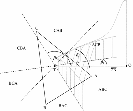
The division of the candidate plane into the six sectors that define the six rankings, and the volume of the wedge (the integral under the spherical bivariate normal distribution centered at \(O\)) that describes the probability that a randomly chosen voter ranks the three candidates in the order ABC
To match the variance of the angles that we determine from observed election data, we parameterize the Dirichlet distribution so that each of the three shares is multiplied by the common constant 73.5008. Dividing the three values in the text by this number yields three shares that sum to 1.
For example, if candidate \(A\) is the winner of voting situation \(R\), then the four pairs of rankings are (ABC, BAC), (ACB, CAB), (BAC, BCA), (CAB, CBA).
In three-candidate elections in which voters must submit full rankings, we treat a truncated ballot for candidate \(X\) as half a ballot for each of the two rankings with \(X \)first. This treatment permits us to examine truncated rankings with two rules, the Kemeny rule and the Coombs rule, that do not permit ballots listing only a single candidate.
The definition of SCC requires that the winner for \(R\) be the unique winner.

References
Arrow K (1951) Social choice and individual values, 1st edn. New York (2nd edn., New Haven, 1963)
Black D (1958) The theory of committees and elections. Cambridge University Press, Cambridge
Brams SJ (1982) The AMS nominating system is vulnerable to truncation of preferences. Not Am Math Soc 29:136–138
Chamberlin JR, Cohen M (1978) Toward applicable social choice theory: a comparison of social choice functions under spatial model assumptions. Am Polit Sci Rev 72:1341–1356
Chamberlin JR, Featherston F (1986) Selecting a voting system. J Polit 48(2):347–369
Condorcet MJAN (1785) “Essai sur l’application de l’analyse à la probabilité des décisions rendues à la pluralité des voix”. L’Imprimerie Royale, Paris
Coombs CH (1964) A theory of data. Wiley, New York
Copeland AH (1951) A ‘reasonable’ social welfare function”. Mimeo, University of Michigan, Department of Mathematics, Seminar on Applications of Mathematics to the Social Sciences
de Borda J-C (1784) Mémoire sur les élections au scrutin”. Histoire de l’Academie Royale des Sciences, Paris
Felsenthal DS (2012) Review of paradoxes afflicting procedures for electing a single candidate. In: Felsenthal DS, Machover M (eds) Electoral systems: paradoxes, assumptions, and procedures. Springer, Berlin, pp 19–91
Fishburn PC (1974a) Paradoxes of voting. Am Polit Sci Rev 68:537–546
Fishburn PC (1974b) On the sum-of-ranks winner when losers are removed. Discret Math 8:25–30
Fishburn PC (1977) Condorcet social choice functions. SIAM J Appl Math 33:469–489
Fishburn PC (1982) Monotonicity paradoxes in the theory of elections. Discret Appl Math 4:119–134
Fishburn PC, Brams SJ (1983) Paradoxes of preferential voting. Math Mag 56:207–214
Gehrlein W (2006) Condorcet’s paradox. Springer, Berlin
Gehrlein W, Lepelley D (2011) Voting paradoxes and group coherence: the Condorcet efficiency of voting rules. Springer, Berlin
Good IJ, Tideman TN (1976) From individual to collective ordering through multidimensional attribute space. Proc R Soc Lond Ser A 347:371–385
Henry M, Mourifié I (2011) Euclidean revealed preferences: testing the spatial voting model. J Appl Econ. doi:10.1002/jae.1276
Hoag CG, Hallett GH (1926) Proportional representation. Macmillan, New York
Kemeny J (1959) Mathematics without numbers. Daedalus 88:577–591
Laslier J-F (2011) Lessons from in situ tests during French elections. In: Dolez B, Grofman B, Laurent A (eds) In situ and laboratory experiments on electoral law reform: French presidential elections. Springer, Heidelberg, pp 90–104
Laslier J-F (2012) And the loser is plurality voting. In: Felsenthal DS, Machover M (eds) Electoral systems: paradoxes, assumptions, and procedures. Springer, Berlin, pp 327–351
Lepelley D, Merlin V (2001) Scoring run-off paradoxes for variable electo-rates. Econ Theory 17:53–80
Merrill S (1984) A comparison of efficiency of multicandidate electoral systems. Am J Polit Sci 28:23–48
Nanson E (1883) Methods of elections. Trans Proc R Soc Vic 19:197–240
Nurmi H (1992) An assessment of voting system simulations. Public Choice 73:459–487
Nurmi H (1999) Voting paradoxes and how to deal with them. Springer, Berlin
Nurmi H (2012) On the relevance of theoretical results to voting system choice. In: Felsenthal DS, Machover M (eds) Electoral systems: paradoxes, assumptions, and procedures. Springer, Berlin, pp 255–274
Plassmann F, Tideman TN (2011) How to assess the frequency of voting paradoxes and strategic voting opportunities in actual elections. Mimeo. Available at http://papers.ssrn.com/sol3/papers.cfm?abstract_id=1911286
Saari DG (2001) Decisions and elections; explaining the unexpected. Cambridge University Press, Cambridge
Smith JH (1973) Aggregation of preferences with variable electorate. Econometrica 41:1027–1041
Stern H (1993) Probability models on rankings and the electoral process. In: Flieger M, Verducci JS (eds) Probability models and statistical analysis for ranking data. Springer, Berlin, pp 173–195
Tideman TN (2006) Collective decisions and voting. Ashgate, Burlington
Tideman TN, Plassmann F (2012) Modeling the outcomes of vote-casting in actual elections. In: Felsenthal DS, Machover M (eds) Electoral systems: paradoxes, assumptions, and procedures. Springer, Berlin, pp 217–251
Young P (1974) An axiomatization of Borda’s rule. J Econ Theory 9:43–52
Young P (1988) condorcet’s theory of voting. Am Pol Sci Rev 82: 1231–1244
Acknowledgments
We thank two anonymous referees for their helpful comments and suggestions. All remaining errors are ours
Author information
Authors and Affiliations
Corresponding author
Appendices
Appendix 1: Simulating elections with the spatial model
1.1 A.1.1 A spatial model of vote-share probabilities
The spatial model of voting represents a conceptualization of the distribution of voter ideal points and the locations of candidates in candidate space. Good and Tideman (1976) describe the philosophy and the technical details of the spatial model that we use; here we summarize its essential elements. Consider the case of \(m\,=\,3\) candidates. There are two sub-cases to be considered. The first is that the three candidates are collinear, that is, all three lie in a single line. In this case, the candidate that is in the middle will not be the last choice of any voter. Since every candidate is the last choice of some voters in the vast preponderance of the results for elections with three candidates that we have seen, we neglect this case and consider the more general case in which the positions of three candidates are not collinear. In this case the locations of the three candidates define a plane, namely the plane that we call candidate space. Label the candidates \(A,\,B\), and \(C\), so that the 3! = 6 different strict rankings are ABC, ACB, CAB, CBA, BCA, and BAC. The six strict rankings form a voting situation that describes how many ballots voters have cast for each of the six rankings.
We assume that the locations of voter ideal points in candidate space follow a circularly symmetric bivariate normal distribution. The probability that a voter chosen at random will place the three candidates in a particular order (e.g., ABC) is the integral of the density function of voter ideal points over the portion of the plane where the order of the distances to the three candidates is the order prescribed by the ranking whose probability is being calculated. The portions of the plane assigned to the six rankings of the three candidates are delineated by the perpendicular bisectors of the line segments connecting pairs of candidates. Figure 3 shows, for specific locations of the three candidates, the division of the candidate plane into the six sectors that define the six rankings. The figure also shows the volume of the triangular wedge (the integral under the spherical multivariate normal distribution centered at \(O)\) whose integral describes the probability that a randomly chosen voter ranks the three candidates in the order ABC.Footnote 34
While there are six degrees of freedom in the locations of the three candidates, there are only four degrees of freedom in the probabilities determined by the integrals. One degree of freedom is lost because, if the positions of the three candidates are rotated around the mode of the distribution of voter ideal points, the pattern of perpendicular bisectors rotates by the same amount, and the integrals are unchanged. A second degree of freedom is lost because, if the locations of the three candidates are moved the same distance toward or away from the point that is equidistant from them, the perpendicular bisectors and hence the integrals are unchanged.
There are different ways to use the remaining four degrees of freedom to describe the structure of the spatial model. We found that the following parameterization makes it easiest to simulate rankings that are very similar to the voting situations that we observe in actual elections. We first place the intersection of the three perpendicular bisectors of the triangle formed by the three candidates (that is, the triangle’s circumcenter \(T\)) at the origin of a coordinate system, and we rotate the coordinate system so that the center of voter ideal points \(O\) is on its horizontal axis. We then use the first degree of freedom for the horizontal distance OT, and the remaining three degrees of freedom for the angles formed by the line \(\overline{OT}\) and the three perpendicular bisectors that describe the boundaries between pairs of the six strict rankings. To simulate data with the spatial model, we adopt distributions for the parameters based on the analysis of real voting data in Plassmann and Tideman (2011). In particular, we assume that \(\overline{OT}\) follows a Weibull distribution with scale parameter \(\alpha \,=\,0.6858\) and shape parameter \(\beta \,=\,2.4608\), and that the three angles follow a Dirichlet distribution with parameters \(\delta _{1}\,=\,26.47,\,\delta _{2}\, =\,23.37\), and \(\delta _{3}~=~23.65\).Footnote 35
1.2 A.1.2 A model of vote-casting outcomes
The spatial model yields a vote share probability \(p_{r}\) for each of the six strict rankings \(r\), with \(\Sigma p_{r}~=~1\). To complete the model of vote-casting, it is necessary to describe the relationship between the vote share probabilities (six real numbers) and the number of ballots that \(n\) voters submit for each of the six rankings (six integers). We assume that the \(p_{r}\)s represent the expected shares of the ballots. We also assume that the distribution of the vector of \(p_{r}\)s does not vary with the size of the electorate. To formalize these assumptions, let \(n_{r}\) be the number of ballots submitted for ranking \(r\), with \(\Sigma n_{r}=n\) and \(r=1,\ldots ,6\), and let \(N_{r}\) be a random variable that describes the distribution of \(n_{r}\). If voters cast their ballots independently of each other, then in a given election in which the expected vote shares are given by a vector of \(p_{r}\)s, the six \(N_{r}\)s follow a multinomial distribution with \(E[N_{r}]= np_{r}\) (and thus \(E[{N_r /n}]=p_r),\,Var[N_{r}]=np_{r}\,(1 - p_{r})\), and Cov [\(N_{r},\,N_{s}]=-np_{r}p_{s}\). One way of accommodating dependent ballots is to assume that the six \(n_{r}\)s follow a multinomial-Dirichlet distribution with \(E[N_{r}]=np_{r},\,Var[N_{r}]=np_{r}(1 - p_{r})\Psi \), and \(Cov[N_{r},\,N_{s}]=- np_{r}p_{s}\Psi \), where \(\Psi = (\psi +n)/(\psi + 1)\). The parameter \(\psi \) describes the additional variance that is introduced through the Dirichlet distribution; in the limit as \(\psi \) approaches infinity, the multinomial-Dirichlet distribution approaches the multinomial distribution. Plassmann and Tideman (2011) show that the multinomial distribution leads to less variation among simulated ballots than what is observed in ballots from actual elections, while the variation among ballots simulated with a multinomial-Dirichlet distribution with \(\psi ~=~330\) is very close to the variation among observed ballots. Thus a specified distribution for the \(p_{r}\)s leads to a distribution of election outcomes, for any size of electorate, that can be parameterized and simulated.
1.3 A.1.3 A model of voter behavior versus a model of vote-casting outcomes
The spatial model can be interpreted either as a model of voter behavior or as part of a model of vote-casting outcomes. It is important to distinguish the two interpretations. When viewed as a model of voter behavior, the task would be to identify the positions of the ideal points in actual elections. Knowledge of these positions would explain why one observes a particular voting situation. The key question would be whether observed voting situation can be interpreted as revealed preferences that provide information about the positions of the ideal points. This question has received considerable attention in the literature; Henry and Mourifié (2011) assess and reject the validity of the spatial model of voting when it is interpreted as a model of voter behavior.
In contrast, when the spatial model serves as a model of vote share probabilities and thus as part of a model of vote-casting outcomes, the focus is on the distribution of voting situations rather than the positions of ideal points. The task is to parameterize the spatial model so that the model of vote-casting outcomes yields a distribution of voting situations that corresponds to the distribution of observed voting situations. Knowledge of the positions of ideal points is not required for this task. Thus our work is neither related to nor affected by the literature on revealed preferences. We adopt the spatial model as a model of vote-casting outcomes solely because, among all contenders for a model of vote share probabilities of which we are aware, it comes closest to describing the distribution of observed voting situations, not because we want to defend it as a model of voter behavior.
Appendix 2: Estimating the frequencies of five voting paradoxes
Let “voting rule \(X\)” be the voting rule for which the frequency of occurrence of a paradox is to be determined. Let \(P\) be the number of occurrences of the paradox, where \(P\,=\,0\) before the first voting situation is drawn. Let \(N\) be the number of voting situations to be drawn.
1.1 A.2.1 The strong lack of monotonicity paradox
-
1.
Use the calibrated spatial model to draw a voting situation \(R\).
-
2.
Use voting rule \(X\) to determine the winner of \(R\).
-
3.
There are four pairs of rankings across which the winner is ranked in consecutive positions.Footnote 36 Consider each of these four pairs in turn, starting with the first pair. If the ranking in which the winner is ranked lower has at least one vote, then decrease the number of votes for that ranking by one and increase the number of votes for the other ranking by 1. Denote the new voting situation by \(R^\prime \). If the ranking in which the winner is ranked lower has no votes, then continue with the next pair of rankings. If this was the fourth pair of rankings, then continue with Step 1.
-
4.
Use voting rule \(X\) to determine the winner of \(R^\prime \).
-
5a.
(Ignoring ties) If voting rule \(X\) chooses different winners for \(R\) and \(R^\prime \), then increment \(P\) by 1. Continue with Step 1.
-
5b.
(Accounting for ties) If voting rule \(X\) chooses either (1) different winners for \(R\) and \(R^\prime \), or (2) the same winner for \(R\) and \(R^\prime \) and the winner is unique for \(R\) but not unique for \(R^\prime \), then increment \(P\) by 1. Continue with Step 1.
-
6.
If \(P\) was not incremented in Step 5, then the following must be true: voting rule \(X\) chooses the same winner for the two voting situations. Continue with Step 3 with a different pair of rankings. After the fourth pair, continue with Step 1.
-
7.
Determine the frequency of occurrence as \(P/N\).
1.2 A.2.2 The strong truncation paradox
Steps 1–2 and 4–7 are the same as in A.2.1
-
3.
Consider each of the six possible strict rankings in turn, starting with the first ranking. Denote this ranking by \(r\). If ranking \(r\) has at least one vote, then decrease the number of votes for ranking \(r\) by one-half. Identify the ranking \(r^\prime \) that has the same highest-ranked candidate as ranking \(r\), and increase the number of votes for ranking \(r^\prime \) by one-half.Footnote 37 Denote the new voting situation by \(R^\prime \). If ranking \(r\) has no votes, then continue with the next ranking. If ranking \(r\) is the sixth ranking, then continue with Step 1.
1.3 A.2.3 The strong no-show paradox
Steps 1–2 and 4–7 are the same as in A.2.1
-
3.
Consider each of the six possible strict rankings in turn, starting with the first ranking. Denote this ranking by \(r\). If ranking \(r\) has at least one vote, then decrease the number of votes for ranking \(r\) by one. Denote the new voting situation by \(R^\prime \). If ranking \(r\) has no votes, then continue with the next ranking. If ranking \(r\) is the sixth ranking, then continue with Step 1.
1.4 A.2.4 Violations of the Subset Choice Consistency (SCC) Condition
Steps 1–2 are the same as in A.2.1
-
3.
If the winner of voting situation \( R\) is not unique, then continue with Step 1.Footnote 38
-
4.
Consider, in turn, each of the two candidates who did not win, starting with the first of these candidates. Eliminate this candidate. Use \(R\) to assemble the voting situation \(R^{\mathrm{short}}\) for the ensuing two-candidate election.
-
5.
Use voting rule \(X\) to determine the winner for \(R^{\mathrm{short}}\) (this is the majority rule winner for all 14 voting rules that we consider).
-
6a.
(Ignoring ties) IF the winner for \(R^{\mathrm{short}}\) is not the same as the winner for \(R\), THEN increment \(P\) by 1. Continue with Step 1.
-
6b.
(Accounting for ties) IF (1) the winner for \(R^{\mathrm{short}}\) is not the same as the winner for \(R\), or (2) the winner for \(R^{\mathrm{short}}\) is not unique (there is a two way tie that involves the winner of \(R)\), THEN increment \(P\) by 1. Continue with Step 1.
-
7.
If \(P\) was not incremented in Step 6, then the following must be true: the winner for \(R^{\mathrm{short}}\) is the same as the winner for \(R\). Continue with Step 4 with the other candidate. After the second candidate, continue with Step 1.
-
8.
Determine the frequency of occurrence as \(P/N\).
1.5 A.2.5 The reinforcement paradox
We examine only the version of the reinforcement paradox for which the two elections under consideration either have the same number of voters or have a number of voters that differs by exactly 1 across the elections. When sampling the elections for the results reported in Table 12, we assumed that the number of voters in each of the two individual elections sum to the number of voters listed in the header of each column.
-
1.
Use the spatial model to draw two voting situations, \(R\) and \(R^\prime \).
-
2.
Use voting rule \(X\) to determine the winners for \(R\) and \(R^\prime \).
-
3.
If the winners of \(R\) and \(R^\prime \) are not the same, then continue with Step 1.
-
4.
Combine \(R\) and \(R^\prime \) to form a new voting situation \(R^{\prime \prime }\).
-
5.
Use voting rule \(X\) to determine the winner for \(R^{\prime \prime }\).
-
6.
EITHER the winners for \(R,\,R^\prime \), and \(R^{\prime \prime }\) are unique, OR some/all winners are not unique but one decides to ignore ties. One of the following must be true:
-
6a.
The winner for \(R^{\prime \prime }\) IS NOT the same as the winner for \(R\) and \(R^\prime \). If true, then increment \(P\) by 1 and continue with Step 1.
-
6b.
The winner for \(R^{\prime \prime }\) IS the same as the winner for \(R\) and \(R^\prime \). If true, then continue with Step 1.
-
6a.
-
7.
Reaching Step 7 implies that the winners for \(R,\,R^\prime \), and \(R^{\prime \prime }\) are not unique and that one decides not to ignore ties. One of the following must be true:
-
7a.
The winner of \(R^{\prime \prime }\) is tied with another candidate and the winners of \(R\) and/or \(R^\prime \) are tied with the same candidate. If true, then continue with Step 1.
-
7b.
The winner of \(R^{\prime \prime }\) is tied with another candidate and the winners of \(R\) and/or \(R^\prime \) are either not tied or tied with a different candidate. If true, then increment \(P\) by 1 and continue with Step 1.
-
7c.
The winner of \(R^{\prime \prime }\) is not tied and the winners of \(R\) and/or \(R^\prime \) are tied with another candidate. If true, then increment \(P\) by 1 and continue with Step 1.
-
7a.
-
8.
Determine the frequency of occurrence as \(P/N\).
Rights and permissions
About this article
Cite this article
Plassmann, F., Tideman, T.N. How frequently do different voting rules encounter voting paradoxes in three-candidate elections?. Soc Choice Welf 42, 31–75 (2014). https://doi.org/10.1007/s00355-013-0720-8
Received:
Accepted:
Published:
Issue Date:
DOI: https://doi.org/10.1007/s00355-013-0720-8