
Abstract
This paper describes the experimental setup, procedure, and results obtained, concerning the dynamics of a body lying on a floor, attached to a hinge, and exposed to an unsteady flow, which is a model of the initiation of rotational motion of ballast stones due to the wind generated by the passing of a high-speed train. The idea is to obtain experimental data to support the theoretical model developed in Sanz-Andres and Navarro-Medina (J Wind Eng Ind Aerodyn 98, 772–783, (2010), aimed at analyzing the initial phase of the ballast train-induced-wind erosion (BATIWE) phenomenon. The experimental setup is based on an open circuit, closed test section, low-speed wind tunnel, with a new sinusoidal gust generator mechanism concept, designed and built at the IDR/UPM. The tunnel’s main characteristic is the ability to generate a flow with a uniform velocity profile and sinusoidal time fluctuation of the speed. Experimental results and theoretical model predictions are in good agreement.
1 Introduction
A wind tunnel equipped with a gust generation mechanism has been developed as part of a research program on the ballast pick-up phenomenon generated by high-speed trains (more specifically, ballast train-induced-wind erosion or BATIWE), to study the initiation of motion of a ballast stone lying on the track due to the aerodynamic force produced by a time-dependent wind. If this force is great enough, the body can start to rotate around the most rearward supporting contact point (RSCP) of the stone. If the stone has some previous sliding motion over the sleeper or other stones in the ballast bed, it is assumed that this sliding motion will be blocked by the physical interference at this RSCP, and only rotation around RSCP will be allowed from this moment onwards. In Sanz-Andres and Navarro-Medina (2010), this motion is modeled by considering the dynamics of the rotation of the body around a pivoting point fixed to the floor, under the effect of the gravity field and the time-dependent aerodynamic loads produced by a non-steady incoming flow. If, due to the aerodynamic moment, the object obtains enough rotation speed, it can start to roll, then begin to jump, hitting the floor and bouncing, and eventually acquiring the vertical speed that is necessary to initiate flight (Quinn et al. 2009). This rotation initiation phase is an intermediate phase between the two stages generally considered, namely, the initial static equilibrium without motion and the final flight (Kwon and Park 2006). In this intermediate phase, both the rotational dynamics of the body and the gust characteristics of the incoming flow should be taken into account in order to determine whether, once the motion is initiated, it leads either to a frustrated motion or to a successful one. To analyze this problem, a non-linear mathematical model has been developed by Sanz-Andres and Navarro-Medina (2010), which can be simplified by linearizing the formulation, based on the consideration that the incoming flow is an almost steady flow changing slightly due to a sinusoidal perturbation.
The train-induced flow field is turbulent, with some singular higher peaks. This can be appreciated in the results of measurements performed on the track reported by Quinn et al. (2009). We assume that the stone will be moved by an individual gust of this turbulent flow. This gust should be both intense and last long enough to be able to move the stone. We also assume that the shape of the singular gust is a sinusoidal peak. It is convenient for the modelization from the analytical point of view and the experimental point of view (to simulate in a gust wind tunnel). In both cases, although the sinusoidal variation is defined for all times, only the interval of time starting at the instant when the net moment acting on the stone becomes positive is considered. Hence, each peak of the sinusoidal variation is individually considered, that is, the sinusoidal variation is seen as a series of individual gusts.
The main goal of the work reported here is to validate the above-mentioned theoretical model by simulating in a wind tunnel this intermediate phase in similar conditions to those considered in the theoretical model. In this regard, an open circuit, closed test section, low-speed wind tunnel with a new sinusoidal gust generator mechanism concept has been built at the IDR/UPM. Speed measurements in the test section have been carried out to determine the wind tunnel performances. The maximum gust frequency achieved is about 10 Hz, and the maximum wind speed is approximately 20 m/s. The test section size is 0.39 m × 0.54 m, which is large enough to meet the size requirements for experiments with stone models. This low-cost, gust wind tunnel can also be used for related studies, such as the starting of soil erosion, initiation of debris flight, or determination of non-steady bluff body drag.
BATIWE is a relatively new phenomenon, but it can be traced back to the flight of wind-borne objects, which in different configurations has received a great amount of interest from the scientific community since the mid-twentieth century. In this regard, three related problems can be outlined: soil eolian erosion (Owen 1964), flying debris (Baker 2007; Lin et al. 2006; Richards et al. 2008), and ballast pick-up by high-speed trains (Kwon and Park 2006). Concerning soil eolian erosion, the chain reaction that appears is of relevance for BATIWE, leading to a process called saltation (Bagnold 1941). The research concerning saltation includes, among others, wind tunnel testing (Rice et al. 1995), 2D numerical simulation (Werner and Haff 1998), studying it as a simulation of the cascade collision and ejection of ions (Ta and Dong 2007), and sand-bed impact tests (Rice et al. 1995; Rice et al. 1996; Werner and Haff 1998). The cascade collision can help to explain the maintenance of saltation, but unfortunately, it does not help to explain the starting process.
In the case of BATIWE, when a high-speed train exceeds a critical speed, it produces a wind speed close to the track high enough to start the motion of the ballast elements, eventually leading to stone rolling (Kwon and Park 2006). If they get enough energy, they can jump and then initiate a saltation-like chain reaction. This chain reaction could appear when the stones that have jumped return to the track floor and hit the resting stones, transmitting to them a part of the momentum that the flying stones have obtained from the wind generated by the train. These high energy impacts give impulse to the hit stones, and some of them start to move, feeding the chain reaction. The expelled stones can produce damage to the train and the infrastructure. Particularly, the initiation of flight of ballast due to the pass of a high-speed train has been studied by Kwon and Park (2006) by performing field and wind tunnel experiments. These authors have also developed a simple mathematical model of the trajectory, once the motion has started, that is, without considering the phase of rotational motion initiation.
Also in relation with BATIWE, Quinn et al. (2009) make reference to the mechanism of initiation of the ballast particle flight. Before the initiation of flight, a roll-jump process has been found with ballast stones by Kwon and Park (2006). As above-mentioned, the initial rotation together with the rolling–jumping phase is an intermediate phase between the initial equilibrium and the final flight, a phase that is more relevant in the case of a time-varying, gusty flow, like the one generated by a passing train.
In Sanz-Andres and Navarro-Medina (2010), a theoretical model of this rotational motion initiation phase has been developed, which takes into account the dynamics of the body and the gust characteristics in order to determine whether, once initiated, the motion leads to either a frustrated motion or a successful one. In order to check this theoretical model, a flow with a sinusoidal perturbation of an otherwise steady wind speed should be obtained in the test section, while keeping the velocity vector direction horizontal, and with some acceptable degree of uniformity in the velocity across the wind tunnel section (uniform velocity profile).
Several studies have been done concerning the design of mechanisms to create a flow with velocity fluctuations in a wind tunnel in order to study the response of structures to gust excitation. However, their characteristics are far from those required by the present study, for several reasons. In the work of Tang et al. (1996), a rotating slotted cylinder mechanism is used, which can produce a controllable single or multiple harmonic gust along lateral and longitudinal combined directions of the wind tunnel, while the harmonic longitudinal gust amplitude depends on the transversal position. However, such a mechanism is not appropriate for the present work because it does not fulfill the uniform velocity profile requirement.
A similar setup, but based on an active control mechanism composed of arrays of plates, airfoils, and velocity sensors, in a two-dimensional wind tunnel, is used to achieve a large-scale turbulent flow whose velocity spectra is fitted to a target one similar to natural wind spectra (Kobayashi and Hatanaka 1992) or to obtain a target time history of the wind velocity (Kobayashi et al. 1994). In these cases, both along-wind and vertical gusts are obtained, the mean velocity is nearly uniform along the lateral direction (as it should be in a two-dimensional wind tunnel) but not along the vertical one, and therefore, a uniform velocity profile is not obtained.
Hermann (1978) developed a fluidic jet control apparatus that consists of a nozzle with elongated plates, which are positioned downstream of the exit port on opposite sides, and two rotating valves for controlling the flow supply. A device with two of these nozzles can be used to provide both transverse and longitudinal gusts, the latter only in the middle plane between the nozzles and not uniformly across the test section as is needed here. Other authors involved in gust generation for wind tunnels have considered the generation of transverse disturbances of the flow but not on modulus variation of otherwise uniform velocity profiles of the wind velocity.
An apparatus for selectively generating transverse wave motion of the air flow in a wind tunnel has been developed by Loftin (1961). This transverse velocity component is achieved by rotating two airfoil vanes positioned in each of the side walls upstream of the test section. Haan and Sarkar (2006) developed an active gust generation mechanism in a wind tunnel, although their aim was to obtain a single step gust, of a large magnitude velocity change within the shortest possible time, but not a sinusoidal one.
Other examples are the gust generator for testing small anemometers has been developed by Hölling et al. (2007), or the active grid system for producing artificial wind speed is reported in Kang et al. (2003). In the present work, to fulfill the above-mentioned requirements (namely, a uniform velocity profile flow, an almost steady speed with a small sinusoidal time fluctuation), an open circuit, low-speed wind tunnel with a new gust generator mechanism concept has been set up at the IDR/UPM.
The contents of this paper are organized as follows. In Sect. 2, the mathematical model developed by Sanz-Andres and Navarro-Medina (2010) is summarized, and the conditions for the starting and continuation of the motion are presented. As the problem is a non-linear one, in order to obtain some useful analytical results, a first-order formulation of the non-linear problem is developed and its solution is obtained, valid for small amplitude motions, which allows us to analyze the influence of the initial conditions in the success of the rotational motion. The sinusoidal fluctuation of speed considered in the linearized problem should also be reproduced in the wind tunnel in order to compare the theoretical model with experimental observations. In Sect. 3, the wind tunnel is described. In Sect. 4, the characteristics and performances of the wind tunnel with sinusoidal gust generation capability, designed to obtain a non-steady flow, are described. In Sect. 5, the experimental setup and some results obtained from experiments performed with stone models are presented, and these data are compared with the theoretical predictions. Finally, in Sect. 6, conclusions are drawn.
2 Summary of the theoretical model
In this section, the mathematical model of Sanz-Andres and Navarro-Medina (2010) on the initiation of the rotational motion of a stone lying on a horizontal plane is summarized. The model is based on the stone dynamics equation, which is formulated taking into account both gravity and aerodynamic forces. These aerodynamic forces are the result of the interaction between the train-generated gust and the stones. Although the aerodynamic forces are non-steady, under appropriate conditions, a quasi-steady aerodynamic load model can be employed. As a result of the analysis, a condition for the start of the motion is obtained, which involves the Tachikawa number (a kind of Froude number). Also, the role of the aerodynamic characteristics of the stone is clarified, which are described in terms of the zero aerodynamic moment line (ZML) of the stone and the aerodynamic moment coefficient, c m.
As the problem is a very complex one, in order to extract some preliminary interesting results, it should be simplified to some suitable extent. Following this line, let us consider the geometry and the nomenclature of the problem displayed in Fig. 1. A stone, which is lying on a horizontal wall, can rotate around the RSCP point A, which is the trailing contact point, due to the action of the aerodynamic loads produced by a time-dependent incoming flow U(t), while restrained by the action of the gravity force. A material line AC, or “chord”, is used as a reference for the several different directions considered. The reference for the aerodynamic loads, the ZML, is the direction of the mean wind that produces zero aerodynamic moment with regard to point A. The dynamics of the stone is described by the equation of the angular acceleration produced by the applied torque:
where I is the moment of inertia with regard to point A; ρ a the air density; A Fp the plan form area; R the characteristic stone dimension (e.g., radius of the sphere circumscribing the stone); c m the coefficient of aerodynamic moment with regard to point A; M p the stone mass; g the acceleration of gravity; d cmA the distance between the center of mass and the pivoting point A; θ cm = θ L + δ Lcm, where δ Lcm is the angle between the ZML and the center of mass line, θ L = β + δ CL, β is the angle between the stone chord and the horizontal plane, δ CL the angle between the stone chord and the ZML; and \( U\left( t \right) = U_{0} f\left( t \right) \), where U 0 is the time-averaged incoming speed, and f(t) is the dimensionless wind speed variation with time. The first term inside the brackets is the aerodynamic moment with regard to point A, assuming a quasi-steady behavior. The second term in Eq. 1 is just the moment of the gravity force, with regard to point A.
In order to write Eq. 1 in dimensionless form, the dimensionless time can be defined as \( T = t/t_{\text{crg}} \), based on the characteristic time of the rotational motion of the body due to the effect of gravity forces, t crg,
thus obtaining
where \( \dot{\theta }_{\text{L}} = \frac{{{\text{d}}\theta_{\text{L}} }}{{{\text{d}}t}} = \frac{1}{{t_{\text{crg}} }}\frac{{{\text{d}}\theta_{\text{L}} }}{{{\text{d}}T}} = \frac{1}{{t_{\text{crg}} }}\theta_{\text{L}}^{\prime } \), and K 0 is the Tachikawa number (corresponding to the mean velocity U 0 and including the factor R/d cmA), defined as
The analysis of the solutions of Eq. 3 is focused on the conditions leading to the starting of the motion. In this regard, the conditions to be fulfilled at a time instant t 0 for the body to start the rotation around point A are: (a) equilibrium of applied moment, \( \theta_{{{\text{L}}0}}^{\prime \prime } = 0 \), from Eq. 3 and (b) increasing acceleration \( \theta_{{{\text{L}}0}}^{\prime \prime \prime } > 0 \). Even though the stone starts to move at t 0 (which is the classic assumption employed in erosion studies), the successful continuation of the motion is not guaranteed. Only if the gust duration and intensity are large enough, the stone will obtain enough energy to overcome the restoring effect of gravity forces. In such a case, when the stone’s center of mass reaches the upper position, the gravity restoring torque disappears, and, if the rotation angle increases further, the restoring character will change to a destabilizing action, leading to a continuation of the motion (thereafter referred to as “successful motion”).
However, if the aerodynamic forces are not able to impulse the stone to reach this highest position, the stone will fall back toward its initial position and, therefore, the rolling motion will be frustrated. The determination of the relationship between the parameters that defines the limit of the initial conditions leading to either a frustrated motion or a successful one is based on Eq. 3. In a general case, the determination of initial conditions leading to successful motion implies the numerical integration of Eq. 3 with a suitable definition of the dimensionless wind variation f(T). Fortunately, before trying to solve this complex problem, it is possible to obtain some very helpful information by analyzing a simplified version of the problem obtained by linearization of Eq. 3 assuming that the angles are small, the wind velocity is high enough, and the gust intensity is small compared with the mean wind speed. That is, \( f(T) = 1 + \varepsilon { \sin }\omega t = 1+ \varepsilon { \sin }\Upomega T,\;\varepsilon \ll 1 \), where ω is the angular frequency and Ω is the dimensionless angular frequency
where t cn = 2π/ω is the period of the sinusoidal gust. The motion can be studied by considering small amplitude deviations Θ from a mean value θ Lm, such that θ L = θ Lm × (1 + εΘ), \( \varepsilon \ll 1 \), where θ Lm is the solution of the equilibrium (\( \theta_{L}^{\prime \prime } = 0 \) in Eq. 1), which coincides with the steady excitation case ε = 0.
Once the solution of the linear version of Eq. 3 is obtained, it can be shown that if the stone is at rest at T = T 0, with increasing acceleration, that is, the initial conditions are \( \Uptheta_{0}^{\prime } = \Uptheta_{0}^{\prime \prime } = 0,\;\Uptheta_{0}^{\prime \prime \prime } > 0 \), the stability condition for the initial condition Θ0 (following Sanz-Andres and Navarro-Medina (2010)) can be written as
with Θ0 < 0, which means that the initial value of θ L, θ L0 (defined as θ L0 = θ Lm(1 + εΘ0)), is smaller than the mean value, θ Lm, by an amount ε|Θ0|θ Lm. c mα is the slope of the curve of the aerodynamic moment coefficient against the angle of attack. In physical variables, condition (6) can be written as
where two limit cases for the gust effect can be identified:
-
Limit L: long-duration gust X → 0 (t cn ≫ t crg), θ LlimL = θ Lm (1 − 2 ε).
-
Limit S: short-duration gust X → ∞ (t cn ≪ t crg), θ LlimS = θ Lm = 1/(K 0 c mα).
In the case of long-duration gusts, the effect is the same as that of a quasi-steady flow, that is, the instantaneous speed can be taken as a permanent speed (1 + ε), and the effect on the aerodynamic moment is proportional to 1 + 2ε. Therefore, the limit value corresponds to that which defines the equilibrium at maximum speed. In the case of short-duration gusts, the limit angle is due to the mean value of the aerodynamic force, as the dynamical system given by Eq. 3 filters out the high frequency gusts. Equation 7 can be rewritten as
where it can be seen that the extreme cases L and S can be displayed as two straight lines in a logarithmic plot (Fig. 2). The limit case S is represented as a fixed line, while the position of the line corresponding to case L depends on the value of ε. The region between both lines represents all feasible configurations leading to the starting of successful motion (for some value of X, \( 0 \le X < \infty \)). The size of this region can be defined by the vertical distance between the two lines, which is \( 2\varepsilon \left( { 1+ \, X} \right)^{ - 1/ 2} {\text{loge}} \).

Variation of the limit angle θ Llim with the parameter K 0 c mα. Long-duration (limit L, X → 0) and short-duration (limit S, X = ∞) gusts
3 Wind tunnel description
To check the results of the theoretical model summarized in Sect. 2, a uniform velocity profile flow with a sinusoidal fluctuation of velocity magnitude, while keeping the velocity vector direction horizontal, is required in the wind tunnel test section. To fulfill these requirements, an open circuit, low-speed wind tunnel has been built at the IDR/UPM (Fig. 3). The maximum gust frequency obtained is approximately 10 Hz, and the maximum wind speed is about 20 m/s. The test section size is 0.39 m × 0.54 m.

Sketch of the wind tunnel with the gust generation system: (1) centrifugal fans; (2) transition chamber; (3) metallic duct structure; (4) and (5) lower and upper test chamber, respectively; (6) test section window; (7) pressure probe rake; (8) gust motor; (9) turning gates and gearwheels; (10) test chamber splitter plate; (11) flow quality conditioning elements; and (12) stone model
Air flow in the wind tunnel is generated by two 0.66 m diameter centrifugal fans (Tecnifan TSA-serie R), powered by two 15 kW electrical motors, controlled by a MOELLER DV6-340-15 k frequency inverter. The fan rotational speed, ω F, is the parameter used to control the mean velocity inside the wind tunnel. Air is propelled by these fans (Fig. 3) through a 0.8 m length transition chamber followed by a 2 m length test chamber. Both chambers are made with wooden plates, which are attached to a metallic duct structure.
The working chamber is 0.8 m height and 0.54 m width; although to meet the goal of obtaining a uniform velocity profile, the chamber is divided vertically into two equal parts by means of a horizontal wooden wall. Each part is of 0.54 m width and 0.39 m height. The gust generation is based on a periodic pressure drop concept applied alternatively to the two contiguous test chambers. To achieve the alternative pressure drop, a turning gate is located at the downstream extreme of each test chamber (Fig. 4) in such a way that the phase angle difference is 90°. Therefore, at the time instant when the upper gate blocks the corresponding cross section, the lower gate is completely open, allowing the air to flow freely. As a consequence, the gust generation system produces a flow that goes alternatively through either the upper or lower chamber.

Picture of the gust generation mechanism: (1) gust motor; (2) chain; (3) gearwheels; (4) gust motor mounting support; (5) metallic duct structure; (6) turning gates; (7) test chamber splitter plate; (8) photoelectric proximity switch; (9) turning gate support tubes fixed to the rotating axis
Each turning gate is composed of two rectangular steel plates 1 mm thick and 380 mm × 520 mm sides, which are screwed to 3 steel support tubes fixed to a rotation axis. The steel plates can be positioned at different places along the support tubes, so that the gate chord can be modified, leading to a larger or smaller test section blockage ratio b rg. The turning gate rotation axes are mounted on bearings. One gearwheel is mounted at one end of each gate axis. These two gears are engaged to each other, and to a third gearwheel mounted on the axis of a direct current electric motor, by using a roller chain. The turning gate rotation frequency, or gust frequency f G, is controlled by the motor, which is a 1120 W Mavilor MO-1000 STD model.
A 355 mm × 301 mm rectangular polymethyl methacrylate window is placed in the lower test chamber wall at the appropriate axial position to allow for good visibility of the stone models during tests (Figs. 5, 6). The lower test chamber can be accessed through a gate placed in the floor to facilitate the mounting of the models. All stone models are mounted on wooden base plates, placed close to the window, on the lower test chamber floor, using the access gate.

Picture of the testing area in wind tunnel, showing the reference total pressure probe (1), the semi-spherical model (2), the total pressure probe rake (3), and the screwed rod (4). The air flow is from left to right

Pictures of the models tested: a hemisphere; b flat plane; c square prism; and d hexagonal prism
At a distance of 300 mm downstream from the test chamber entrance, flow quality conditioning elements are placed in order to obtain fluid flows with different values of turbulence intensity. The configurations or arrangements of these flow quality conditioning elements considered here are:
-
C: a clear entrance (no flow quality enhancement);
-
H: a honeycomb 50 mm wide screen with 5 mm cell size;
-
HG: the previous configuration, adding just downstream from the honeycomb, a 5.2 mm cell square grid of 0.8 porosity, made of 0.7 mm diameter wire; and
-
HF: configuration H, adding upstream from the honeycomb, a 15 mm wide foam screen.
4 Flow quality characterization
To determine the flow quality and wind tunnel performances, the wind speed has been measured using total pressure tubes and pressure transducers. Wind velocity profiles can be obtained by using a 13 total pressure probe rake (see Fig. 5), placed at a distance of 0.82 m from the test chamber entrance, whose 2 mm external and 1 mm internal diameter tubes are connected to a Scanivalve 48J7-289 pressure transducer. The total pressure probes are separated 30 mm from each other, and the height of the lowest probe from the floor is 15 mm. The pressure transducers are previously calibrated by using a Druck DPI 610 LP calibrator. The Scanivalve equipment includes a pressure signal amplifier and a channel selector for changing the measuring pressure probe. Channel control and data acquisition are commanded by a computer running a LabView program. Data processing is based on a Matlab program. The velocity measurements performed by using the Scanivalve equipment are identified by V zSC, where z is the vertical position of the probe (in the reference frame defined in Fig. 3, which is positioned at the entrance of the 2 m long test chamber).
With the purpose of taking speed measurements with a higher signal-to-noise ratio, another total pressure probe is included, called here ‘11ST’, which is placed at z = 108 mm and at x = 850 mm away from the working chamber entrance. The speed measured with the ‘11ST’ probe is referred to as V 11ST hereafter. This probe is a brass 5 mm external and 4 mm internal diameter tube, and it is connected to the high pressure port of a low pressure range differential transmitter (Sensor Technics BTEL5P05D1A) by using an 8 mm external and 4.5 mm internal diameter Teflon tube. The internal diameter of the ‘11ST’ probe is wider than the diameter of the probe connected to the pressure transducer of the Scanivalve system, therefore this large diameter allows for improved measurements to be obtained, taking into account that the larger a tube’s internal diameter, the smaller the pressure signal distortion in unsteady pressure measurements. The sensor pressure range is from −500 to 500 Pa, which is suitable for dynamic pressure measurements inside the test section. The maximum limit of the frequency range of the pressure transmitter is approximately 1,000 Hz, higher than the frequency of the gusts created in the wind tunnel.
There are two static pressure taps, one for the Scanivalve system and the other for the 11ST sensor. Both static pressure taps are placed at the same axial position just below the pressure probe noses and connected to the low pressure ports of the transducers. As the tubes from both static pressure and total pressure taps have the same length, adverse effects such as those due to phase delays in the unsteady pressure measurements are avoided. Besides, for the low frequency range (f G < 10 Hz), this length (0.5 m) is short enough to consider the pressure attenuation small (Iberall 1950).
A photoelectric proximity switch (Sick WT150-N132), which gives a pulse at the vertical position of the turning gate of the lower test chamber, is used to determine the gust frequency f G. The three analog signals, one from the Scanivalve, one from the ‘11ST’ pressure transmitter, and the proximity switch signal, are amplified and converted by an IO Tech ADC 488/16-A converter and then sent to a computer. The sampling data rate is 2 kHz. The vertical profiles of the wind speed horizontal component have been measured in Navarro-Medina (2010) and are uniform enough to consider the experimental results reasonably valid. A more detailed description of the wind tunnel and its performances can also be found in the above-mentioned reference.
In order to characterize the time variation of the wind tunnel speed, the velocity V 11ST (measured by the “11ST” probe) is fitted to a sinusoidal function Y(t) for each configuration case, identified by specific values of the tunnel parameters b rg, f G, and ω F, and for each configuration C, H, HG, and HF. This function is
where V 11STm is the mean speed, V 11STa and b/(2π) the amplitude and the frequency of the gust, respectively, and c the phase angle. The ‘Trust-Region Reflective Newton’ method has been used to obtain the fitted curve. In Fig. 7, the instantaneous speed measured with the 11ST pressure measuring system is shown, together with the sinusoidal fitted curve, and the proximity switch signal, which indicates the time instant of maximum test section blockage. Graphs corresponding to a given configuration, changing only one of the parameters, in order to analyze the influence of mean flow speed (proportional to fan rotational speed ω F), gust frequency (f G), flow conditioning configuration, and gust amplitude (which depends on b rg), respectively, are shown in Fig. 7. The values of parameters of each configuration and their respective plots are collected in Table 1. A good agreement between the time variation of velocity signals and the sinusoidal approximation can be seen. It should be remarked that the valleys of sinusoidal curve occur close to the moments (a little out of phase), in which the lower turning gate is in the vertical position, as expected. By increasing the fan rotational speed ω F, the mean flow speed increases, but the gust amplitude also increases in such a way that the dimensionless amplitude ε increases too, as is shown in Fig. 7a. Varying the gust frequency f G, the mean speed V 11STm, and the gust amplitude V 11STa is not substantially modified, as shown in Fig. 7b. Concerning the influence of the flow conditioning configuration (Fig. 7c), scattering (related to flow turbulence intensity of the stream flow), the mean speed V 11STm, and the gust amplitude V 11STa, decrease successively for the configurations C, H, HG, and HF. An exception is for V 11STm from the clear to honeycomb configurations. By increasing b rg, some reduction in the mean speed and increase in the gust amplitude can be observed (see Fig. 7d).


Variation with the time t of the reference velocity V 11ST (dot line) together with the curve fitting to sinusoidal variation Y (solid line), a increasing the fan speed; b increasing the gust frequency; c changing the flow conditioning configuration; d increasing the gate chord length (or the section blockage ratio). Configuration cases are shown in Table 1
A linear variation with ω F of mean speed V 11STm, and gust amplitude V 11STa, is shown in Figs. 8 and 9, respectively. As is shown in Fig. 8, the mean flow speed for the steady case (where the test section gate is open) is higher than for the cases with gusts (where the test chamber is periodically partially blocked by the turning gates). This difference of mean flow speed, among the steady and gusty cases, is not so great for the HF configuration. An explanation for this fact could be that the pressure drop in the foam screen used in this case, placed only in the lower test chamber entrance, but not in the upper chamber, is large, therefore the air flows easier through the upper chamber than the lower chamber for both the steady and gusty cases. Concerning the gust amplitude, its variation with ω F is generally linear (see the case HF from Fig. 9), although in some cases, there are deviations from the linear variation (i.e., case C from Fig. 9). By increasing ω F, the gust amplitude V 11STa decreases, except for case C when ω F is 900 min−1. In any case, for each successive configuration C, H, HG, and HF, the differences between the curves (V 11STa) decrease.

Variation with fan rotational speed (ω F) of mean reference speed V 11STm, for several gust frequencies (f G = 0, 1.8, 2.9, 4.6 y 7.3 Hz); flow conditioning cases C, H, HG, and HF; and a section blockage ratio b rg = 0.49

Variation with fan rotational speed (ω F) of gust amplitude V 11STa, for several gust frequencies (f G = 0, 1.8, 2.9, 4.6 y 7.3 Hz); flow conditioning cases C, H, HG, and HF; and a section blockage ratio b rg = 0.49
5 Experimental setup and results
5.1 Stone model setup
A set of tests has been conducted in the above-mentioned gust wind tunnel to check the agreement between theoretical predictions and experimental results, namely, the variation of the limit angle θ Llim with the parameter K 0 c mα. In order to meet this goal, some stone models were selected to be tested inside the wind tunnel with the gust generator described above. Some regular shapes were chosen, such as hemi-spherical, flat plate, and both square and hexagonal prisms (Fig. 6). The hemi-spherical model is a 2 mm thick and 100 mm diameter polycarbonate shell with a wooden base plate attached with a hinge to the mounting base on the test chamber floor. The hinge simulates the RSCP point, which remains fixed. The flat plate, made of wood, is square, and both the square and the hexagonal prisms are made of necuron. In Table 2, the mass and dimensions of all stone models are compiled. The angle of attack of the model can be changed by using a screwed rod placed upstream of the hinge (Fig. 5), which allows the experimenter to change the supporting point height. There is a margin of error in the supporting point height of some ±0.8 mm, which is due both to the manual positioning of the zero angle level (±0.4 mm) and to the appreciation of the experimenter of the instant of initiation of the successful motion of the stone model (±0.4 mm), which leads to an equivalent error in the angle of attack of some 2°.
After placing the stone model in a horizontal position, and setting the flow quality and gust amplitude (blockage ratio b rg), each test run is performed by sweeping the parameters mean flow speed (depending on ω F) and gust frequency (f G). Each value of the limit angle θ Llim is obtained by slowly changing the stone model angle of attack, while keeping constant the mean flow speed, and at the same time carefully watching for two phenomena: first the initiation of the stone’s movement (frustrated motion initiations), and then at the limit angle, when the successful motion occurs (the model rotation surpasses the vertical position). For steady cases (f G = 0 Hz), turning gates are blocked at the position that allows the stream to flow freely through the lower test chamber, therefore blocking the upper test chamber.
5.2 Aerodynamic parameters of the stone models
In the first place, the values of the unknown aerodynamic parameters of the model, the slope of the curve of variation of aerodynamic moment coefficient vs the angle of attack, c mα, and the angle between the stone chord and the zero moment line, δ CL (Fig. 1), are needed to calculate the limit angle of the stone’s successful motion initiation, θ Llim. For this purpose, steady wind speed tests have been performed. As an example of the results of those tests, the variation with the angle of attack of the aerodynamic moment coefficient with regard to point A, c m(β), for several cases, is shown in Fig. 10. The cases of hemi-spherical, flat plate, square, and hexagonal prism models are shown in Fig. 10a, b, c, and d, respectively. The values of the function c m(β) are determined by using the moment equilibrium equation, which establishes that the aerodynamic moment is equal to the gravity force moment at a given angle of attack and a given wind speed at the instant of the start of successful motion. It should be noted that the slope of the fitting straight line is taken as c mα and that δ CL = −β 0, where the angle β 0 is defined as c m(β 0) = 0. The values of these parameters should only depend on the model geometry, but in case C (clear entrance), they also depend on the flow quality, as can be seen in Fig. 10a. A possible explanation is that in case C, the turbulence intensity is considerably larger than in the other cases, and non-steady effects can appear, which have an influence in determining of c m(β) due to the difficulty in visually discriminating the instant of successful motion. The variation of the aerodynamic moment coefficient with the angle of attack is quite linear in hemi-spherical and flat plate cases (Fig. 10a, b). For the prismatic models (see Fig. 10c, d), this variation is linear with the angle of attack for angles smaller than a critical one, but it becomes constant for larger angles.

Variation with the angle of attack, β, of the aerodynamic moment coefficient with regard to the model rotating point A, c m (β), for several types of object: a Hemisphere; b flat plate; c square prism; and d hexagonal prism. Flow quality conditioning cases: C clear, H honeycomb, HG honeycomb plus grid, HF honeycomb plus foam. M 0 object mass
5.3 Determination of θ Llim
Once these crucial aerodynamic parameters were determined, tests devoted to the determination of the successful initiation of motion of the hemi-spherical stone model were performed, whose results are plotted in Fig. 11. The limit angle between the horizontal plane and the Zero Moment Line, θ Llim, is plotted against both the mean wind speed U 0, Fig. 11a, and the parameter K 0 c mα, Fig. 11b. Theoretical calculations based on Eq. 7 are also plotted in Fig. 11 together with the experimental results. In the theoretical model, two limit cases were predicted: the low frequency gust case (lower limit) and the steady speed case (upper limit), which coincides with the high frequency gust case. To check this result, three values of the frequency of turning gate rotation are displayed, for both theoretical predictions and experimental results, as follows: the steady case, a low frequency gust and a high frequency one. As presented in Fig. 11, in the high-speed range (or large values of K 0 c mα), the three resultant experimental curves appear in the expected order as predicted by the theoretical model: the steady case curve as the upper limit, the low frequency case curve in the lower position, and the high frequency case curve in the middle. Furthermore, as the velocity increases, experimental results show a better agreement with theoretical predictions, as a consequence of the better accuracy of the linearized model in the high speed, low angle of attack range. In the low speed range, which implies high angles of attack, the predictions of the linearized model are not accurate.

Variation with a mean speed U 0, or b the parameter K 0 c mα, of the angle between the horizontal plane and the Zero Moment Line in the successful motion initiation instant, θ Llim. Experimental results for several values of f G (circles, 0 Hz; squares, 2.9 Hz; diamonds, 7.3 Hz) and theoretical predictions (solid line, 0 Hz; dashed line, 2.9 Hz; dotted line, 7.3 Hz). Case: blockage ratio b rg = 0.69; case H (honeycomb screen); hemisphere; and M 0 = 37 g (model mass)
In Fig. 12, experimental results for the four stone model shapes are displayed in logarithmic plots of the variation of θ Llim versus the parameter K 0 c mα, showing that the curves for the hemi-spherical body and the flat plate are straight lines (Fig. 12a, b). For the prismatic bodies, two regions appear which can be identified by the difference in slope. This fact can be explained taking into account that the form of the aerodynamic moment coefficient variation with the angle of attack also shows two different regions (Fig. 10).

Experimental results. Variation with the parameter K 0 c mα, of the angle between the horizontal plane and the Zero Moment Line at the successful motion initiation instant, θ Llim, for several types of object: a hemisphere, b flat plate, c square prism, and d hexagonal prism. M 0: object mass. f G = 0 Hz (circles), 2.9 Hz (squares), 7.3 Hz (asterisk). Blockage ratio b rg = 0.69. ε: gust semi-amplitude divided by mean speed U 0
5.4 Validity of the similarity parameter K 0 c mα
One interesting point is the analysis of the suitability of using the parameter K 0 c mα to rearrange the experimental results, as suggested by the theoretical model. In this regard, the results obtained with the hemi-spherical model are shown in Fig. 13 at the same gust frequency, but with several flow conditioning configurations in each plot. In the theoretical model, it was found that the limit value of θ L for successful motions of the stone model depends only on the parameter K 0 c mα if ε and Ω are constant. This theoretical prediction is confirmed by the results shown in Fig. 13. The small difference between curves for different flow conditioning configurations (Fig. 13b, c) is a consequence of the limited capacity of the current gust wind tunnel mechanism to keep constant the value of dimensionless amplitude ε along a given curve (whose variation is displayed in the legend of Fig. 13), and also for different configurations.

Experimental results. Variation of the angle between the horizontal plane and the Zero Moment Line in the successful motion initiation instant, θ Llim, with the parameter K 0 c mα for the hemisphere. a f G = 0 Hz; b f G = 2.9 Hz; and c f G = 7.3 Hz. Blockage ratio b rg = 0.69. Case H, honeycomb (circles), case HG, honeycomb plus grid (squares), case HF, honeycomb plus foam (asterisk). ε: gust semi-amplitude divided by mean speed U 0
The value of K 0 c mα in the case of a stone placed on a sleeper can be estimated assuming U 0 = 20 m/s, ρ a = 1.2 kg/m3, M p = 0.1 kg, R = d cmA, A Fp = 16 cm2 and c mα in the range from 1 to 3. The values of K 0 c mα thus obtained are between 0.3 and 2. These values are included in the range of values that give rise to the motion of the stone (Figs. 12, 13). The velocity of the flow acting on the stones has been estimated form the results on page 4 of Quinn et al. (2009).
6 Conclusions
The study of the effect of wind on several bodies lying on a flat floor, a configuration that is a model of one of the phases of the BATIWE phenomenon, has been presented; the main parameters influencing the phenomenon of the starting of the rotational motion have been identified; and the relationship among them that leads to a successful motion has been obtained. Two limits, for long and short-duration gusts, have been identified. To allow for the comparison of the results predicted by the theoretical model with experimental results (based on a uniform flow with sinusoidal gusts), a wind tunnel with a new gust generation mechanism has been set up. A great flexibility has been considered in the wind tunnel design to allow for the change of the parameters involved, the flow quality, and the wind gust amplitude.
The performance of the wind tunnel varying its control parameters has been determined. It has been shown that the vertical profile of the horizontal component of velocity is uniform enough to consider the experimental results valid, although the different vertical profiles of velocity associated with the flow quality conditioning elements should be taken into account when calculating the mean wind speed at the test object location height. Each flow conditioning configuration has been characterized in terms of flow turbulence intensity, mean speed, and gust amplitude. Depending on future aims, for instance, increasing the mean wind speed while keeping constant either the absolute or the dimensionless gust amplitudes, new improvements in the wind tunnel will be needed, such as an active control system. For instance, a good quality gust flow, with different amplitudes and frequencies, can be obtained by using honeycomb plus a foam layer. Otherwise, by not placing screens at the entrance of the test chamber, a somewhat larger noise can also been obtained. The final choice of the appropriate configuration for each test will depend on the flow requirements, such as the mean flow velocity, the frequency and amplitude of the gust, and the high frequency fluctuation background intensity.
The unknown aerodynamic parameters of the tested models, as the slope of the curve of variation of the aerodynamic moment coefficient against the angle of attack, and the angle between the stone chord and the zero moment line have been determined. It has been shown that the variation of the aerodynamic moment coefficient with the angle of attack is quite linear in hemi-spherical and flat plate cases, but for the prismatic models, this variation has two regions. In the first region, for angles smaller than a critical one, the variation is linear with the angle of attack, but it becomes constant for angles greater than a critical value. This behavior has been observed in experiments in the wind tunnel with prismatic stone models.
The theoretical model predicts that the results will be found in the region bound by two limits: the low frequency gust case (lower limit) and the steady speed case (upper limit), which coincides with the high frequency gust case. This prediction has been validated by the experimental results performed with several stone models. Besides, as velocity increases, experimental results have shown a better agreement with the theoretical predictions, which can be explained bearing in mind that the higher the velocity, the lower the starting angle, and consequently, the linear approximation considered in the derivation of the theoretical results is more realistic.
Another conclusion of the theoretical model was that the results depend only on stone and flow parameters grouped as K 0 c mα, which is the Tachikawa number, K 0, times the slope of the curve of variation of the aerodynamic moment coefficient versus the angle of attack, c mα, at a given dimensionless amplitude and gust frequency. This theoretical prediction has been verified by the experimental results.
Concerning the experiments with the stone models, the experimental configuration inside the wind tunnel is similar, but simplified, to the situation on the railway track of a ballast stone lying on a sleeper (or railroad tie). In the wind tunnel configuration, the values of stone characteristics, such as the mass and dimensions of the stone, and its orientation with respect to wind direction. Wind characteristics, such as mean speed, duration and amplitude of a single-frequency gust and turbulence intensity are known and controllable, unlike the situation on the railway track. Indeed, in the real BATIWE problem, the parameters neither have well specified values of size, shape, mass or position, nor are they deterministic (e.g., the gust duration and intensity). However, they can be described with appropriate probability density functions. Therefore, the future work should be based mainly on statistical analysis, while making use of Eqs. 7 or 8 for the stability limits deduced from the present deterministic studies (as advanced in Sanz-Andres and Navarro-Medina 2010).
Abbreviations
- A Fp :
-
Plan form area
- b rg :
-
Blockage ratio of the rotating gates
- C :
-
Flow quality conditioning configuration
- c m :
-
Coefficient of aerodynamic moment with regard to the rearward supporting contact point (RSCP) A (Fig. 1)
Fig. 1 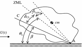
Sketch of the configuration considered. Definition of angles. ZML zero moment line, cm center of mass, AC chord
- c mα :
-
Slope of the curve of the coefficient of the aerodynamic moment with regard to point A versus angle of attack
- d cmA :
-
Distance between the center of mass and the point A
- f(t):
-
Dimensionless fluctuation of wind speed
- f G :
-
Gust frequency
- g :
-
Acceleration of gravity
- h :
-
Wind tunnel test section height
- I :
-
Moment of inertia with regard to point A
- K 0 :
-
Tachikawa number corresponding to the mean wind velocity U 0
- M p :
-
Stone mass
- M 0 :
-
Mass of objects tested in the wind tunnel
- R :
-
Characteristic stone dimension, e.g. radius of the sphere circumscribing the stone
- T :
-
Dimensionless time
- t :
-
Time
- t cn :
-
Characteristic time of the gust, period of the excitation
- t crg :
-
Characteristic time of the stone rotational motion due to gravity
- U(t):
-
Wind speed (Fig. 1)
- U 0 :
-
Mean wind speed
- V 11ST :
-
Reference wind speed in the wind tunnel test section
- V 11STm :
-
Mean reference wind speed
- V 11STa :
-
Amplitude of the reference wind speed fluctuation
- V zSC :
-
Wind speed measured with the Scanivalve equipment probe placed at height z
- V zSCm :
-
Time-averaged wind speed at height z
- V zSCmv :
-
Mean speed across the wind tunnel test section, of time-averaged wind speed at height z
- ω :
-
Angular frequency
- ω F :
-
Rotational speed of the wind tunnel fan
- X :
-
Gust parameter
- x :
-
Longitudinal coordinate of the wind tunnel reference frame (Fig. 3)
- z :
-
Vertical coordinate of the wind tunnel reference frame
- α :
-
Angle of attack, angle between the horizontal plane and a reference line of the stone
- β :
-
Angle between the stone chord and the horizontal plane (Fig. 1)
- δ CL :
-
Angle between the stone chord and the zero moment line (Fig. 1)
- δ Lcm :
-
Angle between the zero moment line and the center of mass line (Fig. 1)
- ε :
-
Dimensionless amplitude of the sinusoidal wind fluctuation
- Ω:
-
Dimensionless angular frequency
- Θ:
-
Stretched angular position of the zero moment line
- Θ0lim :
-
Limit value of initial stretched angular position θ 0 for stable evolution
- ρ a,ρ p :
-
Density of air, of stone, respectively
- θ cm :
-
Angle between the center of mass line and the horizontal plane
- θ L :
-
Angle between the zero moment line and the horizontal plane (Fig. 1)
- θ Llim :
-
Limit value of θ L for stable evolution
- θ Lm :
-
Mean value of θ L
- 0:
-
Initial value (unless otherwise defined)
- limL:
-
Long gust limit
- limS:
-
Short gust limit

References
Bagnold RA (1941) The physics of blown sand and desert dunes. Chapman and Hall, London
Baker CJ (2007) The debris flight equations. J Wind Eng Ind Aerodyn 95:329–353
Haan FL Jr, Sarkar PP (2006) Development of an active gust generation mechanism on a wind tunnel for wind engineering and industrial aerodynamics applications. Wind Struct 9(5):369–386
Hermann V (1978) Fluidic oscillating jet for high frequency gust tunnel. US Patent 4074568
Hölling M, Schulte B, Barth S, Peinke J (2007) Sphere anemometer—a faster alternative solution to cup anemometry. J Phys Conf Ser 75:1–6
Iberall AS (1950) Attenuation of oscillatory pressures in instrument lines. J Res Natl Bur Stand 45:85–108
Kang HS, Chester S, Meneveau C (2003) Decaying turbulence in an active-grid-generated flow and comparisons with large-eddy simulation. J Fluid Mech 480:129–160
Kobayashi H, Hatanaka A (1992) Active generation of wind gust in a two-dimensional wind tunnel. J Wind Eng Ind Aerodyn 41–44:959–970
Kobayashi H, Hatanaka A, Ueda T (1994) Active simulation of time histories of strong wind gust in a wind tunnel. J Wind Eng Ind Aerodyn 53:315–330
Kwon HB, Park CS (2006) An experimental study on the relationship between ballast-flying phenomenon and strong wind under high-speed train. In: Proceedings of 7th world congress on railway research. Montreal
Lin N, Letchford C, Holmes JD (2006) Investigations on plate-type windborne debris, part I, experiments wind tunnel and in full scale. J Wind Eng Ind Aerodyn 94:51–76
Loftin LK (1961) Wind tunnel airstream oscillating apparatus. US Patent 3005339
Navarro-Medina F (2010) Levantamiento de balasto en las líneas de ferrocarril de alta velocidad (in Spanish). Universidad Politécnica de Madrid, Doctoral Thesis
Owen PR (1964) Saltation of uniform grains in air. J Fluid Mech 20(2):225–242
Quinn AD, Hayward M, Baker CJ, Schmid F, Priest JA, Powrie W (2009) A full-scale experimental and modelling study of ballast flight under high speed trains. J Rail Rapid Transit Proc Inst Mech Eng 224(2):61–74
Rice MA, Willetts BB, McEwan IK (1995) An experimental study of multiple grain-size ejecta produced by collisions of saltating grains with a flat bed. Sedimentology 42:695–706
Rice MA, Willetts BB, McEwan IK (1996) Observation of collisions of saltating grains with a granular bed from high-speed cine-film. Sedimentology 43:21–31
Richards PJ, Williams N, Laing B, McCarty M, Pond M (2008) Numerical calculation of the three-dimensional motion of wind-borne debris. J Wind Eng Ind Aerodyn 96:2188–2202
Sanz-Andres A, Navarro-Medina F (2010) The initiation of rotational motion of a lying object caused by wind gusts. J Wind Eng Ind Aerodyn. 98:772–783
Ta WQ, Dong ZB (2007) Simulation on sand grain/bed collision mechanism: cascade collision and ejection. Geomorphology 89:348–357
Tang DM, Cizmas PGA, Dowell EH (1996) Experiments and analysis for gust generator in a wind tunnel. J Aircr 33(1):139–148
Werner BT, Haff PK (1998) The impact process in aeolian saltation: two-dimensional simulations. Sedimentology 35:189–196
Acknowledgments
The study covered in this paper has been carried with financial support from Administracion de Infraestructuras Ferroviarias (ADIF) and Patentes Talgo S.A. The authors would like to thank Miguel Rodriguez from ADIF, and Emilio García and David Pérez Rodriguez from Patentes Talgo S.A. for fruitful discussions and suggestions.
Author information
Authors and Affiliations
Corresponding author
Rights and permissions
About this article
Cite this article
Navarro-Medina, F., Sanz-Andres, A. & Perez-Grande, I. Gust wind tunnel study on ballast pick-up by high-speed trains. Exp Fluids 52, 105–121 (2012). https://doi.org/10.1007/s00348-011-1201-4
Received:
Revised:
Accepted:
Published:
Issue Date:
DOI: https://doi.org/10.1007/s00348-011-1201-4