On the Vanishing Electron-Mass Limit in Plasma Hydrodynamics in Unbounded Media

Abstract

We consider the zero-electron-mass limit for the Navier–Stokes–Poisson system in unbounded spatial domains. Assuming smallness of the viscosity coefficient and ill-prepared initial data, we show that the asymptotic limit is represented by the incompressible Navier–Stokes system, with a Brinkman damping, in the case when viscosity is proportional to the electron-mass, and by the incompressible Euler system provided the viscosity is dominated by the electron mass. The proof is based on the RAGE theorem and dispersive estimates for acoustic waves, and on the concept of suitable weak solutions for the compressible Navier–Stokes system.

1 Introduction

Singular limits arise frequently in the process of model reduction in fluid mechanics. In this paper we consider the limit of vanishing ratio electron mass/ion mass in a hydrodynamic model for plasma confined to an unbounded spatial domain Ω⊂R ³.

1.1 Equations

For a given (constant) density N _i of positively charged ions, the time evolution of the electron density n _e=n _e(t,x) and the electron velocity u=u(t,x) is governed by the system of equations

(1.1)

(1.2)

(1.3)

where m _e is the ratio of the electron/ions mass, p is the electron pressure, Φ is the electric potential, τ is the relaxation time, and $\mbox{$\mathbb{S}$}$ denotes the viscous stress tensor,

$$ \mathbb{S}(\nabla_x\mathbf{u}) = \tilde{\mu}\biggl( \nabla_x\mathbf{u}+ \nabla_x^t \mathbf{u}- \frac {2}{3} \mathrm{div}_x\mathbf{u}\mathbb{I} \biggr),\quad \tilde{\mu}> 0. $$

(1.4)

The interested reader may consult Anile and Pennisi (1992), Jüngel and Peng (2000, 2001) for the physical background and a detailed derivation of the model.

We suppose that the electron velocity satisfies the slip boundary conditions

$$ \mathbf{u}\cdot\mathbf{n}|_{\partial\varOmega} = 0, \bigl[\mathbb{S} ( \nabla_x\mathbf{u}) \mathbf{n}\bigr] \times\mathbf{n}|_{\partial\varOmega} = 0, $$

(1.5)

and the boundary is electrically insulated,

$$ \nabla_x\varPhi\cdot\mathbf{n}|_{\partial\varOmega} = 0. $$

(1.6)

As the underlying spatial domain is unbounded, we also prescribe the far-field behavior:

$$ \mathbf{u}(x) \to0 ,\qquad \varPhi(x) \to0 \quad \mbox{as}\ |x| \to \infty. $$

(1.7)

Our goal is to study the singular limit and identify the limit problem for m _e→0 under the condition

• $\tilde{\mu}\approx m_{\mathrm {e}}$, or

• $\tilde{\mu}/ m_{\mathrm {e}} \to0$ as m _e→0.

1.2 Ill-prepared Initial Data

For m _e=ε ², $\mu_{\varepsilon}= \tilde{\mu}/\varepsilon^{2}$, problem (1.1)–(1.7) is reminiscent of the low Mach (incompressible) limit of the Navier–Stokes system that have been investigated in a number of recent studies, see the survey papers by Danchin (2002), Gallagher (2005), Masmoudi (2006), and Schochet (2005), and the references cited therein. The zero-electron-mass limit for the inviscid fluid was treated recently by Ali and Chen (2011), Ali et al. (2010), see also Chen et al. (2011). In the latter case, it is shown that the system becomes neutral, meaning n _e→N _i, while the limit velocity field v satisfies a damped Euler system

(1.8)

(1.9)

supplemented with the impermeability condition,

$$ \mathbf{v} \cdot\mathbf{n}|_{\partial\varOmega} = 0. $$

(1.10)

In Alì et al. (2010), Chen et al. (2011), the authors consider the periodic boundary conditions and well-prepared initial data

$$n_{\mathrm {e}}(0, \cdot) = N_{\mathrm {i}} + \varepsilon^2 N_{0,\varepsilon}, \qquad \mathbf{u}(0, \cdot) = \mathbf{u}_{0, \varepsilon}, \qquad \mathrm{div}_x \mathbf{u}_{0, \varepsilon} = 0. $$

In this paper, we focus on the ill-prepared data, specifically,

(1.11)

(1.12)

In particular, the gradient part of the velocity field will develop fast oscillations in the asymptotic limit ε→0.

1.3 Spatial Domain

In contrast with (Alì et al. 2010), we consider the physically relevant (unbounded) domains with boundaries. Similarly to Farwig, Kozono, and Sohr (2005), we focus on the class of uniform C ³ domains of type (α,β,K). Specifically, for each point of x ₀∈∂Ω, there is a function h∈C ³(R ²), $\| h \|_{C^{3}(R^{2})} \leq K$, and

$$U_{\alpha, \beta,h} = \bigl\{ (y, x_3) \ | h(y) - \beta< x_3 < h(y) + \beta,\ |y| < \alpha \bigr\} $$

such that, after suitable translation and rotation of the coordinate axes, x ₀=[0,0,h(0)] and

Additional hypotheses imposed on the class of domains are stronger for the inviscid limit, so we consider the two cases separately.

1.3.1 Hypotheses in the Case of Constant Viscosity

Since our method leans essentially on dispersion of acoustic waves, we suppose that

• the point spectrum of the Neumann Laplacian Δ_N in L ²(Ω) is empty,

in particular, the domain Ω must be unbounded. Although the absence of eigenvalues for the Neumann Laplacian represents, in general, a delicate and highly unstable problem (see Davies and Parnovski 1998), there are numerous examples of such domains—the whole space R ³, the half-space, exterior domains, unbounded strips, tube-like domains and waveguides, see D’Ancona and Racke (2010).

1.3.2 Hypotheses in the Case of Inviscid Limit

The absence of eigenvalues for the Neumann Laplacian is apparently not sufficient to carry over the inviscid limit. We need stronger dispersion provided by the so-called L ¹–L ^∞ estimates well known for the acoustic equation in R ³, cf. Sect. 7.1 below. More specifically, we focus on the class of physically relevant domains represented by infinite waveguides in the spirit of D’Ancona and Racke (2010). We suppose that

$$ \varOmega\subset R^3, \qquad \varOmega= B \times R^L ,\quad L=1,2,3, $$

(1.13)

where

(1.14)

Obviously, the domains satisfying (1.13) and (1.14) belong to the class of uniform C ³ domains of type (α,β,K), and the point spectrum of the Neumann Laplacian is empty. A peculiar feature of the present problem is that propagation of acoustic waves is governed by a wave equation of Klein–Gordon type (see Sect. 5), where dispersion is enhanced by the presence of “damping”. In particular, we recover the L ¹–L ^∞ estimates even in the case of infinite tubes (L=1) under the Neumann boundary conditions, see Sect. 7.1.

1.4 Asymptotic Limit

By analogy with the low Mach number limits, we expect the limit velocity to satisfy the incompressible Navier–Stokes system with a Brinkman type damping if μ _ε =const>0, and the Euler system (1.8)–(1.10) in the inviscid limit μ _ε →0.

In comparison with the low Mach number limit, the main difficulty here is the presence of the extra term

$$\frac{1}{\varepsilon^2} n_{\mathrm {e}} \nabla_x\varPhi= \frac{n_{\mathrm {e}} - N_{\mathrm {i}} }{\varepsilon} \nabla_x \Delta^{-1}_{\mathrm {N}} \biggl[ \frac{ n_{\mathrm {e}} - N_{\mathrm {i}} }{\varepsilon} \biggr] + \frac{N_{\mathrm {i}}}{\varepsilon^2} \nabla_x\varPhi $$

in the momentum equation (1.2). While the gradient component $\frac{N_{\mathrm {i}}}{\varepsilon^{2}} \nabla_{x}\varPhi$ can be easily incorporated into the pressure in the limit system, the quantity

$$\frac{ n_{\mathrm {e}} - N_{\mathrm {i}} }{\varepsilon} \nabla_x\Delta^{-1}_{\mathrm {N}} \biggl[ \frac{ n_{\mathrm {e}} - N_{\mathrm {i}} }{\varepsilon} \biggr] $$

should “disappear” in the course of the limit process ε→0. To achieve this, the dispersive estimates based on the celebrated RAGE theorem will be used.

Another difficulty lies in the fact that the quantity

$$\frac{ n_{\mathrm {e}} - N_{\mathrm {i}} }{\varepsilon} \nabla_x\Delta^{-1}_{\mathrm {N}} \biggl[ \frac{ n_{\mathrm {e}} - N_{\mathrm {i}} }{\varepsilon} \biggr] $$

is (known to be) only locally integrable; for global analysis, it must be written in the form

$$\frac{ n_{\mathrm {e}} - N_{\mathrm {i}} }{\varepsilon} \nabla_x\Delta^{-1}_{\mathrm {N}} \biggl[ \frac{ n_{\mathrm {e}} - N_{\mathrm {i}} }{\varepsilon} \biggr] = \frac{1}{\varepsilon^2} \biggl( \mathrm{div}_x( \nabla_x\varPhi\otimes \nabla_x\varPhi) - \frac{1}{2} \nabla_x| \nabla_x\varPhi|^2 \biggr), $$

meaning as an element of the dual space W ^−1,1.

Last but not least, we point out that the analysis of the inviscid limit leans heavily on the fact that the propagation of acoustic waves is governed by the Klein–Gordon wave equation, yielding effective dispersion on the waveguide like domains specified in Sect. 1.3.2.

The paper is organized as follows. In Sect. 2, we introduce the concept of suitable weak solution to system (1.1)–(1.7) that proved to be very convenient for studying the inviscid limits, cf. Feireisl et al. (2010). Section 3 contains the main results. In Sect. 4, we summarize the uniform bounds independent of the scaling parameter ε. Section 5 is devoted to the acoustic equation and the resulting dispersive estimates. Finally, in Sect. 6, we show convergence toward the incompressible Navier–Stokes system in the case of non-degenerate viscosity, while Sect. 7 completes the proof of the inviscid limit.

2 Suitable Weak Solutions

Motivated by the general theory developed by Ruggeri and Trovato (2004), we assume that the electron pressure p satisfies

(2.1)

Next, we introduce the standard Helmholtz decomposition of a vector field v,

$$\mathbf{v} = \mathbf{H}[ \mathbf{v} ] + \mathbf{H}^\perp[\mathbf{v}], $$

with

$$\mathbf{H}^\perp= \nabla_x\varPsi,\qquad\Delta\varPsi= \mathrm {div}_x\mathbf{v}\quad \mbox{in}\ \varOmega,\qquad ( \nabla_x\varPsi- \mathbf{v}) \cdot\mathbf {n}|_{\partial \varOmega} = 0. $$

As shown by Farwig et al. (2005), the linear operator

$$\mathbf{H} \ \mbox{is bounded in} \ L^2 \cap L^q ( \varOmega; R^3 ) \ \mbox{for}\ 2 < q < \infty, \ \mbox{and in}\ L^2 + L^q (\varOmega) \ \mbox{for} \ 1 < q \leq2 $$

as soon as Ω is a C ²-domain of type (α,β,K) introduced in Sect. 1.3. Moreover, the norm of H in the aforementioned spaces depends solely on the parameters (α,β,K). As a matter of fact, the domains considered in the present paper belong to the higher regularity class C ³ for several technical reasons that will become clear in the course of the proof of the main results.

Following Feireisl et al. (2011) we say that a trio n _e, u, Φ is a suitable weak solution to system (1.1)–(1.7) in (0,T)×Ω, supplement with the initial conditions n _e(0,⋅)=n ₀, u(0,⋅)=u ₀ if:

• the functions n _e, u, Φ belong to the regularity class

  

• the equation of continuity (1.1) is satisfied in the sense of renormalized solutions (see DiPerna and Lions 1989),

  

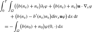
  (2.2)

  for any test function $\varphi\in C^{\infty}_{c}([0,T) \times\overline {\varOmega})$ and any b∈C ^∞[0,∞), $b' \in C^{\infty}_{c}[0,\infty)$;

• the momentum equation (1.2), together with the slip boundary condition (1.5), is satisfied in a weak sense,

  

  (2.3)

  for any test function $\varphi\in C^{\infty}_{c}([0,T) \times\overline {\varOmega}; R^{3})$, φ⋅n|_[0,T)×∂Ω =0;

• the electric potential Φ is given by formula

  $$ \nabla_x\varPhi(s, \cdot) = \nabla_x \varPhi_{0} - \int_0^s \mathbf{H}^\perp[ n_{\mathrm {e}} \mathbf{u}] \, \mathrm{d}t, $$

  (2.4)

  where

  $$ \Delta\varPhi_{0} = n_0 - N_{\mathrm {i}} \quad\mbox{in}\ \varOmega,\qquad \nabla_x \varPhi_0 \cdot \mathbf{n} |_{\partial\varOmega} = 0; $$

  (2.5)

• the relative entropy inequality

  

  (2.6)

  holds for a.a. s∈[0,T] and all test functions r, U such that

  

  where

  

  (2.7)

  with

  $$E(n_{\mathrm {e}}, r) \equiv H(n_{\mathrm {e}}) - H'(r) (n_{\mathrm {e}} - r) - H(r) $$

  and

  $$P \equiv H',\qquad H(n) \equiv n \int_1^n \frac{p(s)}{s^2}\,\mathrm{d}s. $$

It can be deduced from (2.4) that

(2.8)

meaning Φ is a (strong) solution of Poisson equation (1.3). In particular, by virtue of the standard (local) elliptic regularity,

$$ \varPhi(t, \cdot) \in W^{2,5/3}(K) \quad \mbox{for any compact} \ K \subset\overline{\varOmega}. $$

(2.9)

The relative entropy inequality (2.6), introduced in Feireisl et al. (2011), plays the role of a “distance” between a given (weak) solution n _e, u and a pair of “test” functions r, U. The existence of global-in-time suitable weak solutions to the compressible Navier–Stokes system in a bounded spatial domain and the no-slip boundary conditions was proved in Feireisl et al. (2011, Theorem 3.1) with the help of the approximation scheme introduced in Feireisl et al. (2001). Adaptation of the method to the present problem requires only straightforward modifications. Recently, we have shown that (2.6) can be replaced by a weaker stipulation, namely by the standard energy inequality in the form

(2.10)

see Feireisl et al. (2012). More specifically, any weak solution satisfying the energy inequality (2.10) is a suitable weak solution.

The main advantage of working directly with suitable weak solutions is that the relative entropy inequality (2.6) already implicitly includes the stability estimates necessary to perform the inviscid limit.

3 Main Results

We start by introducing the scaled system. To simplify notation, we set m _e=ε ², n _e=n _ε , u=u _ε , Φ=Φ _ε , and $N_{\mathrm {i}} = \overline{n}$—a positive constant. Accordingly, the system of equations (1.1)–(1.3) reads

(3.1)

(3.2)

(3.3)

with the viscous stress

$$ \mathbb{S}_\varepsilon(\nabla_x \mathbf{u}_{\varepsilon }) = {\mu_\varepsilon} \biggl( \nabla_x \mathbf{u}_{\varepsilon }+ \nabla_x^t \mathbf{u}_{\varepsilon }-\frac{2}{3} \mathrm{div}_x\mathbf {u}_{\varepsilon }\mbox{$\mathbb{I}$} \biggr), \quad \mu_\varepsilon> 0. $$

(3.4)

System (3.1)–(3.3) is supplemented with the boundary conditions

(3.5)

(3.6)

and

$$ \mathbf{u}_{\varepsilon }(x) \to0 , \qquad \varPhi_\varepsilon(x) \to0 \quad \mbox{as}\ |x| \to \infty. $$

(3.7)

3.1 Ill-prepared Initial Data

Taking

$$r \equiv\overline{n},\qquad \mathbf{U} \equiv0 $$

as test functions in the relative entropy inequality (2.6) we obtain

(3.8)

where

$$ n_\varepsilon= n_{0,\varepsilon}, \qquad \mathbf{u}_{\varepsilon }(0, \cdot) = \mathbf{u}_{0, \varepsilon} $$

(3.9)

and

$$ \varPhi_{0, \varepsilon} = \Delta^{-1}_{\mathrm{N}} [ n_{0,\varepsilon} - \overline{n}] $$

(3.10)

are the initial data.

Consequently, the initial data must be chosen in such a way that the expression on the right-hand side of (3.8) remains bounded for ε→0. Accordingly, we suppose that

(3.11)

(3.12)

Moreover, the functions N _0,ε must be taken so that $\varPhi_{0,\varepsilon} = \varepsilon\Delta^{-1}_{N} [ N_{0,\varepsilon} ]$ satisfy

$$ \{ \nabla_x\varPhi_{0,\varepsilon} \}_{\varepsilon> 0} \ \mbox{bounded in} \ L^2\bigl(\varOmega;R^3\bigr). $$

(3.13)

3.2 Asymptotic Limit for Positive Viscosity Coefficients

Our first result concerns the asymptotic limit in the case μ _ε =μ>0.

Theorem 3.1

Let Ω⊂R ³ be an (unbounded) C ³-domain of type (α,β,K) specified in Sect. 1.3 and such that the point spectrum of the Neumann Laplacian Δ_N in L ²(Ω) is empty. Suppose that the viscosity coefficient μ _ε =μ>0 is independent of ε and that the pressure p satisfies (2.1). Let {n _ε ,u _ε ,Φ _ε } _ε>0 be a sequence of suitable weak solutions to the scaled system (3.1)–(3.7), emanating from the initial data satisfying (3.11)–(3.13).

Then

$$ \mathrm{ess} \sup_{t \in(0,T)} \| n_{\varepsilon }- \overline{n} \|_{L^2 + L^{5/3}(\varOmega)} \leq\varepsilon c, $$

(3.14)

and, at least for a suitable subsequence,

$$\mathbf{u}_{0,\varepsilon} \to\mathbf{U}_0 \quad \mbox{\textit{weakly in}}\ L^2 \bigl(\varOmega;R^3 \bigr), $$

(3.15)

for any compact K⊂Ω, where U is a weak solution to the incompressible (damped) Navier–Stokes system in (0,T)×Ω,

(3.16)

(3.17)

with

$$ \mathbf{U} \cdot\mathbf{n} |_{\partial\varOmega} = 0, \qquad \bigl[ \mathbb{S}(\nabla_x\mathbf{U}) \mathbf{n}\bigr] \times \mathbf{n}|_{\partial\varOmega} = 0, $$

(3.18)

and

$$ \mathbf{U}(0, \cdot) = \mathbf{H}[\mathbf{U}_0]. $$

(3.19)

Remark 3.1

Momentum equation (3.17), together with the slip boundary conditions (3.18) and the initial condition (3.19), are understood in the weak sense, specifically, the integral identity

(3.20)

for any test function $\varphi\in C^{\infty}_{c}([0,T) \times\overline {\varOmega}; R^{3})$, div _x φ=0, φ⋅n| _∂Ω =0.

3.3 Inviscid Limit

Our second result concerns the case of vanishing viscosity coefficient μ _ε ↘0. In this case, the limit velocity field is expected to satisfy the incompressible Euler system (1.8)–(1.10). As is well known, this system possesses a local-in-time solution

$$ \mathbf{v} \in C\bigl([0,T_{\max}); W^{k,2}( \varOmega)\bigr),\qquad \nabla_x\varPi\in C\bigl([0,T_{\max}); W^{k-1,2}(\varOmega)\bigr) $$

(3.21)

provided

$$\mathbf{v}(0, \cdot) = \mathbf{v}_0 \in W^{k,2}( \varOmega), \quad k > 5/2,\ \mathrm{div}_x\mathbf{v}_0 = 0,\ \mathbf{v}_0 \cdot \mathbf{n}|_{\partial\varOmega} = 0, $$

and provided Ω=R ³, Ω is a half-space, or Ω is an (exterior) domain with compact boundary. The life-span T _max depends solely on $\| \mathbf{v}_{0} \|_{W^{k,2}(\varOmega;R^{3})}$, see Alazard (2005), Isozaki (1987), Secchi (1985), among others. As a matter of fact, the damping term $\frac{1}{\tau} \mathbf{v}$ in (1.9) may extend the life-span of regular solutions, in particular if the initial data are small in comparison with 1/τ. In a very interesting recent paper, Chae (2004) showed that a smooth solution of (1.8)–(1.10) exists globally in time provided Ω=R ³, and $\tau< T^{\mathrm{E}}_{\max}$, where $T^{\mathrm{E}}_{\max}$ is the life span of the regular solution of the undamped Euler system emanating from the same initial data.

Theorem 3.2

In addition to hypotheses of Theorem 3.1, assume that Ω⊂R ³ is an infinite waveguide specified in Sect. 1.3.2. Moreover, we suppose that

$$\mu_\varepsilon\searrow0, $$

and that the initial data satisfy

$$N_{0,\varepsilon} \to N_0 \quad \mbox{(\textit{strongly}) \textit{in}}\ L^2( \varOmega),\qquad \mathbf{u}_{0,\varepsilon} \to\mathbf{u}_0 \quad \mbox{(\textit{strongly}) \textit{in}} \ L^2 \bigl(\varOmega;R^3 \bigr) $$

as ε→0, where

$$\mathbf{v}_0 = \mathbf{H}[\mathbf{u}_0] \in\ W^{k,2} \bigl(\varOmega;R^3 \bigr) , \quad k > 5/2. $$

Moreover, suppose that the damped Euler system (1.8)–(1.10), with the initial datum v ₀, possesses a regular solution v defined on a time interval [0,T _max) satisfying (3.21).

Then

$$ \mathrm{ess} \sup_{t \in(0,T)} \| n_{\varepsilon }- \overline{n} \|_{L^2 + L^{5/3}(\varOmega)} \leq\varepsilon c, $$

(3.22)

and

$$\mathrm{ess} \sup_{t \in(0,T_{\mathrm{loc}})} \bigg\Vert\mathbf{H} \biggl[ \sqrt{ \frac{n_{\varepsilon }}{{\overline{n}}}} \mathbf{u}_{\varepsilon } \biggr] - \mathbf {v} \bigg\Vert_{L^2 (\varOmega;R^3)} \to0, $$

$$\sqrt{\frac{n_{\varepsilon }}{{\overline{n}}}} \mathbf{u}_{\varepsilon }\to\mathbf {v} \quad \mbox{\textit{in}}\ L^{q} \bigl(0,T_{\mathrm{loc}}; L^2 \bigl(K; R^3 \bigr) \bigr)\ \mbox{\textit{for any compact}}\ K \subset\varOmega, \ 1 \leq q < \infty, $$

for any T _loc<T _max, T _loc≤T.

Remark 3.2

The proof of Theorem 3.2 leans essentially on the L ¹–L ^∞ bounds for acoustic waves established in Sect. 7.1. Thus the conclusion of Theorem 3.2 remains valid as soon as these bounds are available. Note that Isozaki (1987) established similar estimates on exterior domains in R ³.

The rest of the paper is devoted to the proof of Theorems 3.1 and 3.2.

4 Uniform Bounds

For the ill-prepared initial data, all desired uniform bounds follow from the energy inequality (3.8). Introducing the essential and residual parts of a quantity h,

where

we get the following list of estimates:

(4.1)

(4.2)

$$ \begin{array}{rcl} \mathrm{ess} \displaystyle\sup_{t \in(0,T)} \bigg\Vert\biggl[ \displaystyle\frac{ n_{\varepsilon }- \overline{n} }{\varepsilon} \biggr]_{\mathrm{ess}} (t, \cdot) \bigg\Vert_{L^2(\varOmega)} &\leq& c , \\[12pt] \mathrm{ess} \displaystyle\sup_{t \in(0,T)} \int_{\varOmega} [n_{\varepsilon }]^{5/3}_{\mathrm{res}} (t,\cdot ) \,\mathrm{d} x \leq\varepsilon^2 c, \end{array} $$

(4.3)

$$ \mathrm{ess} \sup_{t \in(0,T)} \int_{\varOmega} [1]_{\mathrm{res}} (t, \cdot) \,\mathrm{d} x \leq \varepsilon^2 c, $$

(4.4)

and

$$ \mu_\varepsilon\int_0^T \int _{\varOmega} \bigg\vert\nabla_x\mathbf {u}_{\varepsilon }+ \nabla_x\mathbf{u}_{\varepsilon }^t - \frac{2}{3} \mathrm {div}_x\mathbf{u}_{\varepsilon }\mbox{$\mathbb{I}$} \bigg\vert^2 \,\mathrm{d} x \, \mathrm{d} t\leq c, $$

(4.5)

where all generic constants are independent of ε.

Estimates (4.3)–(4.5) can be combined to deduce a bound on the velocity field in the Sobolev space L ²(0,T;W ^1,2(Ω;R ³)), which is relevant in the proof of Theorem 3.1. To this end, we report the following version of Korn’s inequality, which may be of independent interest.

Proposition 4.1

Let Ω⊂R ³ be a C ²-uniform domain of type (α,β,K) introduced in Sect. 1.3.

Then there exists δ>0, depending solely on the parameters (α,β,K), such that

(4.6)

for any measurable set V, |V|<δ, and for all w∈W ^1,2(Ω;R ³).

Proof

In view of the standard decomposition technique and partition of unity, it is enough to show (4.6) on each set

$$U^-_{\alpha, \beta, K} = \bigl\{ (y, x_3) \ | h(y) - \beta< x_3 < h(y) ,\ |y| < \alpha \bigr\}. $$

Revoking the result (Bucur and Feireisl 2009, Proposition 4.1), we have

(4.7)

As a matter of fact, the constant c in (4.7) depends only the Lipschitz constant of the function h and width of U ⁻ given in terms of α, β.

Furthermore, we have

$$| U^-_{\alpha, \beta, K} | \geq2 \delta> 0 $$

for a certain δ(α,β,K)>0. In particular,

$$|U^- \setminus V| > \delta\quad \mbox{for any measurable set}\ V, \ |V| < \delta. $$

Now, arguing by contradiction, we construct sequences

$$h_n \to h \quad \mbox{in} \ C^1 \bigl( |y| \leq\alpha \bigr), $$

$$\{ V_n \}_{n=1}^\infty,\quad |V_n| < \delta, $$

and

$$\{ \mathbf{w}_n \}_{n=1}^\infty, \quad \|\mathbf{w}_n \|_{W^{1,2}(U^-_n;R^3)} = 1, $$

such that

$$\biggl( \bigg\Vert\nabla_x\mathbf{w}_n + \nabla_x^t \mathbf{w}_n - \frac{2}{3} \mathrm{div}_x\mathbf{w}_n \mbox {$\mathbb{I}$} \bigg\Vert^2_{L^2(U^-_n; R^{3 \times3})} + \int_{U^-_n \setminus V_n} | \mathbf{w}_n|^2 \,\mathrm{d} x \biggr) \to0 \quad \mbox{as}\ n \to \infty. $$

Because the domains $U^{-}_{n}$ are uniformly Lipschitz, we can extend w _n as $\tilde{\mathbf{w}}_{n}$ on the cylinder

$$U = \bigl\{ (y, x_3) \, | \, |x_3| < 2 + \beta+ \alpha K, \ |y| < \alpha \bigr\} $$

in such a way that

$$\| \tilde{\mathbf{w}}_n \|_{W^{1,2} (U; R^3)} \leq c(\alpha, \beta, K) \| \mathbf{w}_n \|_{W^{1,2}(U^-_n; R^3)}. $$

Since W ^1,2(U;R ³) is compactly embedded into L ²(U;R ³), we may use (4.7) to deduce that

$$\tilde{\mathbf{w}}_n \to\mathbf{w}\quad\mbox{in} \ W^{1,2} \bigl(U; R^3 \bigr), $$

where

(4.8)

On the other hand,

$$ \int_U 1_{U^-_n \setminus V_n} | \mathbf{w}_n|^2 \, \mathrm{d} x\to \int _U \chi|\mathbf{w}|^2 \, \mathrm{d} x= 0, $$

(4.9)

where

$$1_{U^-_n \setminus V_n} \to\chi\quad\mbox{weakly-(*) in} \ L^\infty (\varOmega), \ \chi\geq0, \ \int_{U} \chi\ \mathrm{d} x> 0. $$

However, relation (4.8) implies that w is a (nonzero) conformal Killing vector (see Reshetnyak 1994) vanishing, by virtue (4.9), on a set of positive measure, which is impossible. □

Thus, finally, taking V the “residual set”, V=supp[1]_res we may combine the estimates (3.8), (4.4), and (4.5) with Proposition 4.1 to conclude that

$$ \mu_\varepsilon\int_0^T \| \mathbf{u}_{\varepsilon }\|^2_{W^{1,2}(\varOmega ;R^3)} \, \mathrm{d} t\leq c. $$

(4.10)

5 Acoustic Equation

As already pointed out, the essential piece of information necessary to carry out the asymptotic limit is contained in the oscillatory component of the velocity field responsible for propagation of acoustic waves. Introducing new variables

$$N_\varepsilon= \frac{n_{\varepsilon }- \overline{n}}{\varepsilon}, \qquad \mathbf{V}_\varepsilon= n_{\varepsilon }\mathbf{u}_{\varepsilon } $$

we can formally rewrite system (3.1) and (3.2) in the form

$$ \varepsilon\partial_t N_\varepsilon+ \mathrm{div}_x\mathbf {V}_\varepsilon= 0, $$

(5.1)

(5.2)

supplemented by the boundary condition

$$\mathbf{V}_\varepsilon\cdot\mathbf{n}|_{\partial\varOmega} = 0. $$

The system (5.1) and (5.2) is usually called the acoustic equation, see Lighthill (1978). Its (rigorous) weak formulation reads

$$ \int_0^T\!\!\int_{\varOmega} ( \varepsilon N_\varepsilon\partial_t \varphi+ \mathbf{V}_\varepsilon \cdot\nabla_x\varphi) \,\mathrm{d} x \, \mathrm{d} t= - \varepsilon\int_{\varOmega} N_{0,\varepsilon} \varphi(0, \cdot) \,\mathrm{d} x $$

(5.3)

for any $\varphi\in C^{\infty}_{c}([0,T) \times\overline{\varOmega})$, and

(5.4)

for any $\varphi\in C^{\infty}_{c}([0,T) \times\overline{\varOmega };R^{3})$, ∇ _x φ⋅n| _∂Ω =0. Moreover, we rewrite

Furthermore, it follows directly from the uniform bounds established in (3.8)–(4.5) that (5.4) can be written as

(5.5)

for any $\varphi\in C^{\infty}_{c}([0,T) \times\overline{\varOmega };R^{3})$, ∇ _x φ⋅n| _∂Ω =0, where

$$ \bigl\{ \mbox{$\mathbb{G}$}^1_\varepsilon\bigr \}_{\varepsilon> 0} \quad \mbox{is bounded in}\ L^\infty\bigl(0,T; L^1\bigl(\varOmega; R^{3 \times3}\bigr)\bigr), $$

(5.6)

and

$$ \bigl\{ \mbox{$\mathbb{G}$}^2_\varepsilon\bigr \}_{\varepsilon> 0} \quad \mbox{is bounded in}\ L^2\bigl(0,T; L^2\bigl(\varOmega; R^{3 \times3}\bigr)\bigr). $$

(5.7)

5.1 Neumann Laplacian

At this stage, it is convenient to rewrite the acoustic system (5.3) and (5.5) in terms of a single self-adjoint operator ${\mathcal{A}}$ in L ²(Ω), specifically,

$$\mathcal{A} = - p'(\overline{n}) \Delta_N + \overline{n} \mbox {$\mathbb{I}$}, $$

with

Given the regularity of the boundary ∂Ω, it can be shown that

(5.8)

Furthermore, since Ω is of uniform C ³-class, the classical elliptic theory yields

$$ {\mathcal{D}}\bigl(\mathcal{A}^2\bigr) \subset C^{2 + \nu} \cap W^{2, \infty} (\overline{\varOmega}) $$

(5.9)

for a certain ν>0. We remark that all we need is only uniform C ^2+ν-regularity of the boundary instead of C ³.

5.2 Acoustic Equation—Abstract Formulation

In view of (5.8) and (5.9), and the uniform bounds established in (5.6) and (5.7), the acoustic equations (5.3) and (5.5) can be written in concise form:

$$ \int_0^T \int _{\varOmega} ( \varepsilon N_\varepsilon\partial_t \varphi+ \mathbf{V}_\varepsilon \cdot\nabla_x\varphi) \,\mathrm {d} x \, \mathrm{d} t= - \varepsilon\int_{\varOmega} N_{0,\varepsilon} \varphi(0, \cdot) \,\mathrm{d} x $$

(5.10)

for any $\varphi\in C^{\infty}_{c}([0,T) \times\overline{\varOmega})$, and

(5.11)

for any $\varphi\in C^{1}([0,T); {\mathcal{D}}(\mathcal{A}^{2}))$, with

$$ \{ F_\varepsilon\}_{\varepsilon> 0}\ \mbox{bounded in}\ L^2\bigl(0,T; L^2(\varOmega)\bigr). $$

(5.12)

Indeed, in view of the bounds (5.6), (5.7), and 5.9,

$$\varphi\mapsto\int_{\varOmega} \bigl( \mbox{$\mathbb {G}$}^1_\varepsilon+ \mbox{$\mathbb{G}$}^2_\varepsilon \bigr) (t,\cdot) : \nabla^2 \varphi \,\mathrm{d} x $$

can be viewed as a bounded linear form on the Hilbert space ${\mathcal{D}}(\mathcal{A}^{2})$; whence, by Riesz representation theorem

$$\int_{\varOmega} \bigl( \mbox{$\mathbb{G}$}^1_\varepsilon+ \mbox {$\mathbb{G}$}^2_\varepsilon \bigr) (t,\cdot) : \nabla^2 \varphi \,\mathrm{d} x = \int_{\varOmega} \mathcal{A}^2 \bigl[f_\varepsilon(t,\cdot) \bigr] \mathcal{A}^2 [\varphi] \,\mathrm {d} x \equiv\int _{\varOmega} F_\varepsilon(t, \cdot) \mathcal{A}^2 [ \varphi] \,\mathrm{d} x. $$

Thus, using the standard variation-of-constants formula, we obtain

(5.13)

(5.14)

where Z _ε is interpreted as

(5.15)

in particular,

(5.16)

Note that the spectrum of the operator $\mathcal{A}$ is the half-line $[\overline{n}, \infty)$.

5.3 Application of RAGE Theorem

With the explicit formulas (5.13) and (5.14) at hand, we are ready to show local energy decay for N _ε and the acoustic waves represented by the gradient component H ^⊥[V _ε ]. To this end, we employ the following version of the celebrated RAGE theorem, see Cycon et al. (1987, Theorem 5.8):

Theorem 5.1

Let H be a Hilbert space, ${A}: {\mathcal{D}}(A) \subset H \to H$ a self-adjoint operator, C:H→H a compact operator, and P _c the orthogonal projection onto the space of continuity H _c of A, specifically,

$$H = H_{\mathrm{c}} \oplus\mathrm{cl}_H \bigl\{ \mathrm{span} \{ w \in H \ | \ w \ \mbox{\textit{an eigenvector of}} \ A \} \bigr\}. $$

Then

$$ \bigg\Vert\frac{1}{\tau} \int_0^\tau \exp(-\mathrm{i} tA ) C P_{\mathrm{c}} \exp( \mathrm{i} tA ) \, \mathrm{d} t \bigg\Vert_{{\mathcal{L}}(H)} \to0 \quad \mbox{\textit{as}}\ \tau \to\infty. $$

(5.17)

We apply Theorem 5.1 to H=L ²(Ω), $A = - \sqrt {{\mathcal{A}}}$, $C = \chi^{2} G(\mathcal{A})$, with $\chi\in C^{\infty}_{c} (\varOmega)$, χ≥0. In accordance with hypotheses of Theorem 3.1, the point spectrum of $\mathcal{A}$ is empty, and we deduce that

$$ \int_0^T \bigg\Vert\chi G( \mathcal{A}) \exp\biggl( \mathrm{i} \sqrt{ \mathcal{A} } \frac{t}{\varepsilon} \biggr) [X] \bigg\Vert^2_{L^2(\varOmega)} \, \mathrm{d} t\leq\omega(\varepsilon) \| X \|_{L^2(\varOmega)}^2, $$

(5.18)

where ω(ε)→0 as ε→0. In particular, going back to (5.13) and (5.14) we may infer that

$$\biggl\{ t \mapsto\int_{\varOmega} N_\varepsilon(t, \cdot) G( \mathcal{A} )[\varphi] \,\mathrm{d} x \biggr\} \to0 \quad \mbox{in}\ L^2(0,T), $$

and, similarly,

$$\biggl\{ t \mapsto\int_{\varOmega} \mathbf{V}_\varepsilon\cdot \nabla_x \bigl( G( \mathcal{A} )[\varphi] \bigr) \,\mathrm{d} x \biggr\} \to0 \quad \mbox{in}\ L^2(0,T) $$

as ε→0 for any $G \in C^{\infty}_{c}(\overline{n}, \infty )$, $\varphi \in C^{\infty}_{c}({\varOmega})$. Thus, by means of a density argument,

$$ N_\varepsilon\to0 \quad \mbox{in}\ L^q\bigl(0,T; \bigl(L^2 + L^{5/3}\bigr)_{\mathrm{weak}\mbox{-}(*)}(\varOmega)\bigr)\ \mbox{for any} \ 1 \leq q < \infty, $$

(5.19)

while

(5.20)

6 Compactness of the Solenoidal Part—Proof of Theorem 3.1

In this section, we complete the proof of Theorem 3.1. To begin, we remark that relation (3.14) follows directly from (4.3), while (4.10) implies that

$$ \mathbf{u}_{\varepsilon }\to\mathbf{U}\quad\mbox{weakly in}\ L^2\bigl(0,T; W^{1,2}\bigl(\varOmega;R^3\bigr) \bigr), $$

(6.1)

at least for a subsequence as the case may be. Moreover, the vector field U is solenoidal and satisfies the impermeability condition U⋅n| _∂Ω =0.

Next, the uniform bounds (4.2) and (4.3), together with the standard elliptic theory, yield

(6.2)

which, combined with (5.19), yields

(6.3)

Taking $\varphi= C^{\infty}_{c}((0,T) \times\varOmega;R^{3})$, div _x φ=0, as a test function in the momentum equation (2.3) and making use of (6.3), we deduce that

$$ \bigl\{ \mathbf{H}[n_{\varepsilon }\mathbf{u}_{\varepsilon }] \bigr \}_{\varepsilon> 0} \ \mbox {is precompact in}\ C_{\mathrm{weak}\mbox{-}(*)}\bigl([0,T]; L^2 + L^{5/4}\bigl(\varOmega; R^3\bigr)\bigr). $$

(6.4)

Indeed the only quantity term reads

$$\frac{1}{\varepsilon^2} n_{\varepsilon }\nabla_x\varPhi_\varepsilon= \frac {\overline{n}}{\varepsilon^2} \nabla_x \varPhi_\varepsilon+ \frac{n_{\varepsilon }- \overline{n}}{\varepsilon} \nabla_x\frac {\varPhi_\varepsilon}{\varepsilon}, $$

where the former term is a gradient, while the latter satisfies (6.3).

Putting together (5.20), (6.1), (6.4), with (3.14), we deduce the desired conclusion

$$ \mathbf{u}_{\varepsilon }\to\mathbf{U} \quad \mbox{(strongly) in} \ L^2\bigl((0,T) \times K; R^3\bigr) \ \mbox{for any compact}\ K \subset\varOmega. $$

(6.5)

With relations (6.3) and (6.5) at hand, it is not difficult to perform the limit ε→0 in the weak formulation of momentum equation (3.2) to obtain (3.20).

We have proved Theorem 3.1.

7 Zero Viscosity Limit—Proof of Theorem 3.2

Our ultimate goal is to prove Theorem 3.2. The basic tool here is the relative entropy inequality (2.6) satisfied by the suitable weak solutions. Taking n _e=n _ε , u=u _ε , $r = \overline{n}$ in the rescaled variant of (2.6) we obtain

(7.1)

with

(7.2)

Furthermore, we take

$$\mathbf{U} = \mathbf{U}_{\varepsilon, \delta} = \mathbf{v} + \nabla_x \varPsi_{\varepsilon, \delta}, $$

where v is the (unique) solution of the damped Euler system (1.8)–(1.10), emanating from the initial data v ₀=H[u ₀], and ∇ _x Ψ _ε,δ mimics the oscillatory part of the velocity field. Specifically, we take

$$ \varepsilon\partial_t s_{\varepsilon, \delta} + \Delta \varPsi_{\varepsilon, \delta} = 0, $$

(7.3)

(7.4)

which is nothing other than a slightly modified homogeneous part of the acoustic system (5.10) and (5.11). The initial data are taken in the form

(7.5)

where the brackets [⋅] _δ denote a suitable regularization operator specified in Sect. 7.1 below.

Keeping (7.3)–(7.4) in mind, we can rewrite the remainder (7.2) in the form

(7.6)

Moreover, we compute

and

$$\int_{\varOmega} \frac{1}{2} n_\varepsilon \partial_t |\nabla_x \varPsi_{\varepsilon, \delta} |^2 \,\mathrm{d} x = \int_{\varOmega } \frac{1}{2} (n_\varepsilon- \overline{n}) \partial_t |\nabla_x \varPsi_{\varepsilon, \delta} |^2 \,\mathrm{d} x + \int_{\varOmega} \frac{1}{2} \overline{n} \partial_t |\nabla_x \varPsi_{\varepsilon, \delta} |^2 \,\mathrm{d} x, $$

where, by virtue of (7.3) and (7.4),

Next, we have

where

$$\frac{1}{\varepsilon} \int_{\varOmega} \Delta\varPsi_{\varepsilon ,\delta} N_\varepsilon \,\mathrm{d} x = - \int_{\varOmega} \partial_t s_{\varepsilon,\delta} N_\varepsilon \,\mathrm{d} x. $$

Finally,

Summing up the previous considerations we may infer that

(7.7)

where

7.1 Dispersive Estimates of the Oscillatory Component

Our goal is to show that solutions s _ε,δ , Ψ _ε,δ of the homogeneous “acoustic” equations (7.3) and (7.4) decay to zero in the L ^∞ norm as ε→0 for any positive time t. To this end, we start with the total energy balance

(7.8)

yielding, in particular, existence and uniqueness of (weak) solutions to problem of (7.3) and (7.4) provided the initial data are smooth and decay sufficiently fast for |x|→∞.

Taking advantage of the special geometry of waveguides, we consider the functions w _k (z), z∈B—the eigenfunctions of the Neumann Laplacian −Δ_N,B in the (bounded) domain B⊂R ^3−L:

The smoothing operators [g] _δ , g=g(x), x=[y,z] are defined as

$$ [g]_\delta(y,z) = \sum_{0 \leq k < 1/\delta} \kappa_\delta(y) * \bigl( \psi_\delta(y) A_k [g](y) \bigr) w_k(z), $$

(7.9)

where

$$A_k[g] (y) = \frac{1}{|B|} \int_B g(y,z) w_k(z) \, \mathrm{d}z, $$

$\psi_{\delta}\in C^{\infty}_{c}(R^{L})$ is a cut-off function,

$$0 \leq\psi_\delta\leq1, \ \psi_\delta(y) = \left \{ \begin{array}{l@{\quad}l} 1 & \mbox{for}\ |y| < 1/\delta, \\[3pt] 0 & \mbox{for}\ |y| > 2/\delta, \end{array} \right . $$

and κ _δ is a family of standard regularizing kernels in the y-variable.

A short inspection of (7.3) and (7.4) yields

$$ s_{\varepsilon, \delta} (t,x) = \exp\biggl( \frac{t}{2\tau} \biggr) \tilde{s}_{\varepsilon, \delta} \biggl( \frac{t}{\varepsilon}, x \biggr), $$

(7.10)

where $\tilde{s}_{\varepsilon, \delta}$ is the unique solution of the Klein–Gordon equation

$$\partial^2_{t,t} \tilde{s}_{\varepsilon, \delta} - p'(\overline{n}) \Delta\tilde{s}_{\varepsilon, \delta} + \biggl( \overline{n} - \frac{1}{4} \frac{\varepsilon^2}{\tau_2} \biggr) \tilde{s}_{\varepsilon, \delta} = 0,\qquad\nabla_x \tilde{s}_{\varepsilon, \delta} \cdot \mathbf{n}|_{\partial\varOmega } = 0, $$

emanating from the initial data

$$ \tilde{s}_{\varepsilon, \delta} (0, \cdot) = \frac{1}{\overline{n}} [N_{0,\varepsilon}]_{\delta},\ \partial_t \tilde{s}_{\varepsilon, \delta} (0, \cdot) = - \Delta [\varPsi_{0,\varepsilon}]_\delta. $$

(7.11)

Consequently, thanks to the specific choice of the smoothing operators (7.9), solutions $\tilde{s}_{\varepsilon, \delta}$ take the form

$$\tilde{s}_{\varepsilon, \delta}(t,x) = \sum_{0 \leq k \leq1/\delta} S_{k, \varepsilon, \delta} (t,y) w_k(z), $$

where S _k (t,⋅) solve the Klein–Gordon equation

$$ \partial^2_{t,t} S_{k,\varepsilon, \delta} - p'(\overline{n}) \Delta_y S_{k,\varepsilon, \delta} + \biggl( \overline{n} - \frac{1}{4} \frac {\varepsilon^2}{\tau^2} + p'( \overline{n}) \lambda_k \biggr) S_{k,\varepsilon, \delta} = 0 $$

(7.12)

for y belonging to the “flat” space R ^L, and with the initial data uniquely determined through (7.11). Thus, employing the standard L ¹–L ^∞ estimates for the Klein–Gordon equation (7.12) (see for instance Lesky and Racke 2003, Lemma 2.4), we have

Going back to (7.10) we may infer that

$$ \big\| s_{\varepsilon, \delta}(t, \cdot) \big\|_{L^\infty(\varOmega)} \leq \omega(t_0, \varepsilon, \delta),\quad t \in[t_0, T], \ t_0 > 0, $$

(7.13)

and, using (7.3),

$$ \big\| \Delta\varPsi_{\varepsilon, \delta}(t, \cdot) \big\|_{L^\infty (\varOmega)} \leq\omega(t_0, \varepsilon, \delta),\quad t \in[t_0, T], \ t_0 > 0, $$

(7.14)

where ω(t ₀,ε,δ)→0 if ε→0 for any fixed t ₀>0, δ>0.

Finally, we claim the standard energy bounds

$$ \| \nabla_x\varPsi_{\varepsilon, \delta} \|_{L^\infty (0,T;W^{m,2}(\varOmega;R^3))} \leq c (m, \delta), $$

(7.15)

$$ \| s_{\varepsilon, \delta} \|_{L^\infty(0,T;W^{m,2}(\varOmega ;R^3))} \leq c(m, \delta), \quad m = 0,1,\dots, $$

(7.16)

where the constants are independent of ε for any fixed δ>0.

7.2 Asymptotic Limit ε→0

Our next goal is to let ε→0 in (7.7), and, in particular, in the remainder Q _ε,δ .

• 1. We have

  

  where

  

  and

  

  Since

  $$n_{\varepsilon }\mathbf{u}_{\varepsilon }= [ \sqrt{ n_{\varepsilon }} ]_{\mathrm{ess}} \sqrt{n_{\varepsilon }} \mathbf{u}_{\varepsilon }+ [\sqrt{ n_{\varepsilon }}]_{\mathrm{res}} \sqrt{n_{\varepsilon }} \mathbf{u}_{\varepsilon }, $$

  where, by virtue of the estimates (4.1) and (4.3),

  $$[\sqrt{n_{\varepsilon }}]_{\mathrm{ess}} \sqrt{n_{\varepsilon }} \mathbf{u}_{\varepsilon }\to \overline{n} \mathbf{U} \quad \mbox{weakly-(*) in}\ L^\infty \bigl(0,T; L^2 \bigl( \varOmega;R^3 \bigr) \bigr),\ \mathrm{div}_x\mathbf{U} = 0, $$

  while

  $$[\sqrt{n_{\varepsilon }}\,]_{\mathrm{res}} \sqrt{n_{\varepsilon }} \mathbf{u}_{\varepsilon }\to0 \quad \mbox{in}\ L^\infty \bigl(0,T; L^{5/4}(\varOmega) \bigr), $$

  we get

  $$\mathrm{ess} \sup_{t \in(0,T_{\mathrm{loc}})} \bigg\vert\int_{\varOmega} n_{\varepsilon }\nabla_x \varPi\cdot\mathbf{u}_{\varepsilon } \, \mathrm{d} x \bigg\vert\to0 \quad \mbox{for}\ \varepsilon\to0. $$

  Similarly, we use (7.15) to observe that

  $$\biggl\{ t \mapsto\int_{\varOmega} \nabla_x\varPi\cdot \nabla_x\varPsi_{\varepsilon, \delta} \,\mathrm{d} x \biggr\} \to0 \quad \mbox{in}\ L^2(0,T_{\mathrm{loc}})\ \mbox{as} \ \varepsilon\to0 $$

  for any fixed δ>0.

  Thus we conclude that

  

  (7.17)

  where

  $$ h^1_{\varepsilon, \delta} \to0 \quad \mbox{in} \ L^2(0,T_{\mathrm{loc}}) \ \mbox{as}\ \varepsilon\to0. $$

  (7.18)

• 2. Taking advantage of the fact that div _x v=0 we can write

  $$\int_{\varOmega} n_{\varepsilon }\partial_t \nabla_x\varPsi_{\varepsilon, \delta} \cdot \mathbf{v} \,\mathrm{d} x = \varepsilon\int_{\varOmega} N_\varepsilon\partial_t \nabla_x\varPsi_{\varepsilon, \delta} \cdot\mathbf{v} \,\mathrm{d} x, $$

  where ε∂ _t ∇ _x Ψ _ε,δ can be expressed by means of (7.4). Using (7.15) and (7.16) we conclude that

  $$ \bigg\vert \int_{\varOmega} n_{\varepsilon } \partial_t \nabla_x\varPsi_{\varepsilon, \delta} \cdot \mathbf{v} \,\mathrm{d} x \bigg\vert= h^2_{\varepsilon, \delta}, $$

  (7.19)

  with

  $$ h^2_{\varepsilon, \delta} \to0 \quad \mbox{in}\ L^2(0,T_{\mathrm{loc}})\ \mbox{as}\ \varepsilon\to0. $$

  (7.20)

• 3. Using (7.14) and (7.15), we show that

  

  (7.21)

  with

  $$ h^3_{\varepsilon, \delta} \to0 \quad \mbox{in}\ L^2(0,T_{\mathrm{loc}}) \ \mbox{as}\ \varepsilon\to0. $$

  (7.22)

• 4. Now,

  

  (7.23)

• 5. Next, in accordance with (4.3) and (7.14), (7.15),

  

  (7.24)

• 6. Finally, using (5.19), (6.2), and (6.3), we infer that

  $$ \bigg\vert \int_{\varOmega} N_\varepsilon \nabla_x\biggl( \frac{ \varPhi_\varepsilon}{\varepsilon} \biggr) \cdot\mathbf{U}_{\varepsilon, \delta } \,\mathrm{d} x \bigg\vert = h^5_{\varepsilon, \delta} \to0 \quad \mbox{in}\ L^2(0,T) \ \mbox {as}\ \varepsilon\to0. $$

  (7.25)

Using estimates (7.17)–(7.25) in (7.7) we conclude that

(7.26)

where

$$ h^6_{\varepsilon, \delta} \to0 \ \mbox{in} \ L^2(0,T_{\mathrm{loc}}) \quad \mbox{as} \ \varepsilon\to0. $$

(7.27)

Now, we claim that

$$\mathrm{ess} \sup_{t \in(0,T)} \bigg\Vert\sqrt{ \frac{ E(n_{\varepsilon }, \overline{n})}{\varepsilon^2} } - \sqrt{ \frac{p'(\overline{n})}{ 2 \overline{n}}} N_\varepsilon \bigg\Vert_{L^{4/3}(\varOmega)} \to0 \quad \mbox{as}\ \varepsilon\to0. $$

Indeed we have

where

while

Consequently, relation (7.26) can be written in the form

(7.28)

with

$$h^7_{\varepsilon, \delta} \to0 \quad \mbox{in}\ L^2(0,T_{\mathrm{loc}}) \ \mbox{as}\ \varepsilon\to0. $$

Applying Gronwall’s lemma we therefore get

where

Thus, letting ε→0 we obtain

$$ \mathrm{ess} \sup_{\varepsilon\to0} \sup_{s \in(0, T_{\mathrm{loc}})}\int _{\varOmega} \biggl( \frac{1}{2} n_\varepsilon| \mathbf{u}_{\varepsilon }- \mathbf {v} - \nabla_x \varPsi_{\varepsilon, \delta} |^2 \biggr) (s, \cdot) \, \mathrm{d} x \le \chi(\delta), $$

(7.29)

where the function χ is determined in terms of the initial data, and χ(δ)→0 as δ→0.

7.3 Asymptotic Limit δ→0

Letting δ→0 in (7.29) we may infer that

$$ \mathbf{H}[\sqrt{n}_{\varepsilon }\,\mathbf{u}_{\varepsilon }]\to \sqrt{\overline{n}}\, \mathbf{v}\quad\mbox{in $L^{2}\bigl(0,T_{\mathrm{loc}};L^{2} \bigl(K;R^{3}\bigr)\bigr)$}, $$

(7.30)

$$ \mathbf{H}^\perp[\sqrt{n}_{\varepsilon }\, \mathbf{u}_{\varepsilon }]\to0 \quad\mbox{in $L^{2}\bigl(0,T_{\mathrm{loc}};L^{2} \bigl(K;R^{3}\bigr)\bigr)$} $$

(7.31)

for any compact K⊂Ω.

The relations (7.30) and (7.31) complete the proof of Theorem 3.2.

References

Alazard, T.: Incompressible limit of the nonisentropic Euler equations with the solid wall boundary conditions. Adv. Differ. Equ. 10(1), 19–44 (2005)
Alì, G., Chen, L.: The zero-electron-mass limit in the hydrodynamic model for plasmas. Nonlinearity 24, 2745–2761 (2011)
Alì, G., Chen, L., Jüngel, A., Peng, Y.-J.: The zero-electron-mass limit in the hydrodynamic model for plasmas. Nonlinear Anal. 72, 4415–4427 (2010)
Anile, A.M., Pennisi, S.: Thermodynamics derivation of the hydrodynamical model for charge transport in semiconductors. Phys. Rev. B 46, 186–193 (1992)
Bucur, D., Feireisl, E.: The incompressible limit of the full Navier–Stokes–Fourier system on domains with rough boundaries. Nonlinear Anal., Real World Appl. 10, 3203–3229 (2009)
Chae, D.: Remarks on the blow-up of the Euler equations and the related equations. Commun. Math. Phys. 245(3), 539–550 (2004)
Chen, L., Chen, X., Zhang, C.: Vanishing electron mass limit in the bipolar Euler–Poisson system. Nonlinear Anal., Real World Appl. 12(2), 1002–1012 (2011)
Cycon, H.L., Froese, R.G., Kirsch, W., Simon, B.: Schrödinger Operators: With Applications to Quantum Mechanics and Global Geometry. Texts and Monographs in Physics. Springer, Berlin (1987)
Danchin, R.: Zero Mach number limit for compressible flows with periodic boundary conditions. Am. J. Math. 124, 1153–1219 (2002)
D’Ancona, P., Racke, R.: Evolution equations in non-flat waveguides (2010). arXiv:1010.0817
Davies, E.B., Parnovski, L.: Trapped modes in acoustic waveguides. Q. J. Mech. Appl. Math. 51(3), 477–492 (1998)
DiPerna, R.J., Lions, P.-L.: Ordinary differential equations, transport theory and Sobolev spaces. Invent. Math. 98, 511–547 (1989)
Farwig, R., Kozono, H., Sohr, H.: An L q-approach to Stokes and Navier–Stokes equations in general domains. Acta Math. 195, 21–53 (2005)
Feireisl, E., Novotný, A., Petzeltová, H.: On the existence of globally defined weak solutions to the Navier–Stokes equations of compressible isentropic fluids. J. Math. Fluid Mech. 3, 358–392 (2001)
Feireisl, E., Novotný, A., Petzeltová, H.: Suitable weak solutions to the compressible Navier–Stokes system: from compressible viscous to incompressible inviscid fluid flows. Preprint (2010)
Feireisl, E., Novotný, A., Sun, Y.: Suitable weak solutions to the Navier–Stokes equations of compressible viscous fluids. Indiana Univ. Math. J. 60, 611–632 (2011)
Feireisl, E., Jin, B.J., Novotný, A.: Relative entropies, suitable weak solutions, and weak-strong uniqueness for the compressible Navier–Stokes system. J. Math. Fluid Mech. (2012). doi:10.1007/s00021-011-0091-9
Gallagher, I.: Résultats récents sur la limite incompressible. In: Séminaire Bourbaki, vol. 2003/2004. Astérisque 299, Exp. No. 926, vii, 29–57 (2005)
Isozaki, H.: Singular limits for the compressible Euler equation in an exterior domain. J. Reine Angew. Math. 381, 1–36 (1987)
Jüngel, A., Peng, Y.-J.: A hierarchy of hydrodynamic models for plasmas. Zero-electron-mass limits in the drift-diffusion equations. Ann. Inst. Henri Poincaré, Anal. Non Linéaire 17(1), 83–118 (2000)
Jüngel, A., Peng, Y.-J.: A hierarchy of hydrodynamic models for plasmas. Quasi-neutral limits in the drift-diffusion equations. Asymptot. Anal. 28(1), 49–73 (2001)
Lesky, P.H., Racke, R.: Nonlinear wave equations in infinite waveguides. Commun. Partial Differ. Equ. 28, 1265–1301 (2003)
Lighthill, J.: Waves in Fluids. Cambridge University Press, Cambridge (1978)
Masmoudi, N.: Examples of singular limits in hydrodynamics. In: Dafermos, C., Feireisl, E. (eds.) Handbook of Differential Equations, III. Elsevier, Amsterdam (2006)
Reshetnyak, Yu.G.: Stability Theorems in Geometry and Analysis. Mathematics and Its Applications, vol. 304. Kluwer Academic, Dordrecht (1994). Translated from the 1982 Russian original by N.S. Dairbekov and V.N. Dyatlov, and revised by the author, Translation edited and with a foreword by S.S. Kutateladze
Ruggeri, T., Trovato, M.: Hyperbolicity in extended thermodynamics of Fermi and Bose gases. Contin. Mech. Thermodyn. 16, 551–576 (2004)
Schochet, S.: The mathematical theory of low Mach number flows. Math. Model. Numer. Anal. 39, 441–458 (2005)
Secchi, P.: Nonstationary flows of viscous and ideal incompressible fluids in a half-plane. Ric. Mat. 34(1), 27–44 (1985)
Acknowledgements
The work of E.F. was supported by Grant 201/09/0917 of GA ČR as a part of the general research programme of the Academy of Sciences of the Czech Republic, Institutional Research Plan AV0Z10190503.
The work of A.N. was partially supported by the general research programme of the Academy of Sciences of the Czech Republic, Institutional Research Plan AV0Z10190503.
Author information
Authors and Affiliations
Corresponding author
Additional information
Communicated by Robert V. Kohn.
Rights and permissions
About this article
Cite this article
Donatelli, D., Feireisl, E. & Novotný, A. On the Vanishing Electron-Mass Limit in Plasma Hydrodynamics in Unbounded Media. J Nonlinear Sci 22, 985–1012 (2012). https://doi.org/10.1007/s00332-012-9134-5
Received:
Accepted:
Published:
Issue Date:
DOI: https://doi.org/10.1007/s00332-012-9134-5