
Abstract
In this article a semi-analytical approach is employed to obtain dimensionless heat transfer correlations for forced convection from isothermal circular cylinders with active ends and different aspect ratios \( (l/d \le 8) \) in laminar axial air flows. Then, using the present results and previous works, the modeling is extended to higher aspect ratios \( (l/d \ge 8) \)) as long as the entire flow field remains completely laminar. Validations of the present work are done not only with the available data on drag coefficients but with previous works for long cylinders with inactive ends and long spheroids. Two general correlations are also developed for a rough estimate of forced convection heat transfer from isothermal cylinders with active ends and arbitrary aspect ratios in the range of \( \frac{1}{2} \le \frac{l}{d} \le 8 \) and \( l/d \ge 8 \).
1 Introduction
Forced convection heat transfer from isothermal or isoflux bodies (cylinder, sphere, cone or cube) is an important problem in science and engineering. A diverse range of applications are typically encountered, including heat transfer from printed circuit boards with low profile chip-on-board packages, cooling of electronic packages, transformers, thermal spreaders, cooling or heating of food items, heat exchangers or packed beds designs. Forced convection heat transfer from spheres has been studied extensively. However, similar works for other geometries such as cuboids or blunt cylinder bodies are very few, if none. A cursory inspection of available literature reveals the preponderance of studies involving the flows of air, i.e. with a Prandtl number value of 0.7, for example see [1–3]. Pop et al. [4] studied the steady incompressible laminar mixed convection boundary layer flow along a rotating vertical slender cylinder with an isothermal wall. They solved transformed coupled nonlinear partial differential equations numerically using the Keller box method. Richelle et al. [5] examined momentum and thermal boundary layers along a yarn of circular cross section in an axial flow for two types of boundary conditions: semi-infinite body and continuous moving surface, using finite difference scheme. Agarwal et al. [6] investigated momentum and thermal boundary layers for power-law fluid over a thin needle numerically under wide range of kinematic and physical conditions. Wiberg and Lior [7] measured local convective heat transfer coefficient on a two-diameter long cylinder in an axial flow of air. The Reynolds number based on the cylinder diameter was between 8.9 × 10⁴ and 6.17 × 10⁵. Sawchuk and Zamir [8] presented a quasi-similar solutions for boundary layer on a circular cylinder in axial flows using a Keller-box numerical scheme; their solution cover a wide range of cylinder radii from very small (needle case) to very large (Blasius case). Bourne and Davies [9] developed a method of calculating the distribution of rate of heat transfer into a laminar incompressible boundary layer from the surface of a cylinder being at a constant temperature and the flow parallel to the cylinder axis. Seban and Bone [10] gave a solution for the case of the laminar boundary layer of an incompressible fluid on the exterior of a cylinder with flow parallel to the cylinder axis. They evaluated the local skin-friction and heat transfer coefficients and compared them with the similar parameters for the flow over a flat plate; the effect of the curvature is shown to be significant in some practical cases. Nowak and Stachel [11] studied the heat transfer process on the external wall of a heated cylinder for laminar axial flows under high pressure conditions, experimentally. Their investigations were aimed at determination of the limits of existence of mixed convection and explanation of the influence of free convection on the disturbances of heat transport during laminar flow of a medium. They also demonstrated the intensification of heat transfer process occurring during a flow under conditions of high pressures. Besides, some experimental investigations have been performed for estimation of drag coefficients of a cylinder for different situations [12]. It includes drag coefficient as a function of length to diameter ratio in incompressible axial flows, drag coefficient of a cylinder in subsonic flow as a function of Mach number and estimation of drag and pressure forces on a cylinder in axial flow for Mach numbers between 0.5 and 8.
In this article, laminar forced convection heat transfer from isothermal cylinders of different aspect ratios, in axial fluid flows, is studied through a semi-analytical method. To fulfill this, Nu–Re relations for different aspect ratios, namely 1/2, 1, 2, 4, 8 are presented. In addition, a general correlation for an estimate of forced convection heat transfer from a cylinder with \( \frac{1}{2} \le \frac{l}{d} \le 8 \) is also given. Then, using the obtained results and some previous works the modeling is extended to higher aspect ratios (\( l/d \ge 8 \)) as long as all flow field remains completely laminar.
1.1 Governing equations
For incompressible Newtonian fluid with constant properties and neglecting viscous dissipation term, the simplified energy equation becomes [1]:
where T is temperature, t time, k, ρ and c are thermal conductivity, density and specific heat, respectively. \( \nabla^{2} \) is the Laplacian operator and \( \frac{DT}{Dt} \) is material derivative of temperature. For heat transfer in continuous fluid it is possible to simplify Eq. 1 when flow Peclet number (Pe) is large. For high Peclet number the temperature varies only in thin layer adjacent to the particle. In this region the gradient of temperature normal to the surface is much larger than the gradient parallel to the surface. The thin thermal boundary layer approximation consists of neglecting diffusion parallel to the surface and retaining only the term involving the derivative normal to the surface on the right-hand side of Eq. 1. Formally this requires Pe → ∞, which for most particular situations means Pr → ∞ for any finite Reynolds number. This approximation is often reasonable down to Pr of order unity. The body shape and the appropriate boundary layer coordinates are sketched in Fig. 1. The x coordinate is parallel to the surface while the y coordinate is normal to the surface. The distance from the axis of symmetry to the surface is R. Equation 1 subjected to the thin thermal boundary layer approximation then becomes [1]:
With boundary conditions:
Here u x and u y are velocity components in the direction of x and y, respectively. T s is particle surface temperature and T ∞ is the flow temperature. In the thin layer adjacent to the particle surface the overall continuity equation may be written as [1]:
Since we only require u x and u y near the surface, the following approximation may be used.
where ζ s is the surface vorticity, given by:
This is so, because \( (\partial u_{y} /\partial x)_{y = 0} = 0 \) for all points on the body surface. Combination of Eqs. 2–7 yields an equation which may be solved to give temperature profiles from which heat transfer rate may be found. The average Nusselt number may be obtained from [1]:
where
Here X M is the maximum value of X and A is the body surface area. Also, d e and A e are the diameter and surface area of the volume equivalent sphere, respectively. Besides, h is the convection heat transfer coefficient and U is the external flow velocity.
2 Methodology
Equation 9 has been used for evaluating Nusselt number of cylinders with aspect ratios of: 1/2, 1, 2, 4, 8 in axial incompressible flows of air. Here, as an example, the procedure is explained for a cylinder with l/d = 1; to do so, Eq. 9 may be rewritten as:
In the above equation, A is the lateral surface area of the cylinder.
Based on the parameters shown in Fig. 2, the following relations can be written:
Substituting Eq. 20 in Eq. 17,
Based on Fig. 2, one can write:
Now, by substituting Eq. 22 in Eq. 18, one gets:
To evaluate an average Nusselt number from Eq. 13, the integral of this equation should be calculated, first. In contrast to Ξ that can be expressed as a mathematical function for simple geometries, ζ s should be estimated numerically. For this reason, flow field around cylinders was solved numerically for different Reynolds numbers. The calculations will lead to have the values of ζ s as a function of X which in turn give the required average Nusselt number values.
Two-dimensional flow of an incompressible fluid with a uniform velocity over a cylinder, of diameter d placed in an infinite medium is simulated by considering the flow in a tubular domain with the cylinder symmetrically on the tube axis. Slip boundary conditions, uniform velocity inlet and outflow were prescribed on the walls, left cross-section area and right cross-section of the tube, respectively. No-slip boundary condition was also considered on the cylinder surface. The length and diameter of the tubular domain are L and D; the cylinder is situated at an up stream distance of s (Fig. 3).

Mathematical model and domain
2.1 Numerical scheme
Because of axisymmetry, in the present numerical modeling the grid needs to be generated only in the half of the radial plane of the domain with axisymmetry boundary condition on the axis of the tube. A domain independence study has been carried out so the selected domain is large enough to include all the effects of body on the flow.
A non-uniform grid was generated by dividing computational domain into 5 sub-domains. This has the advantage that grid points can be clustered in the regions of large gradients and relatively coarse in the regions of minor interest. Figure 4 shows the schematic representation of non-uniform computational grid structures near the cylinder.

Schematic representation of non-uniform computational grid of cylinder
The finite volume method on a staggered grid has been used to discretize and solve the governing equations with an implicit scheme. The pressure terms are discretized using standard scheme and the momentum terms are discretized using the first order upwind. SIMPLE algorithm was employed to solve the equations. The final equations were solved using Gauss–Seidel iterative algorithm [13].
3 Results
3.1 Grid independency study
To study the grid independency, the average Nusselt numbers were calculated for different grids; for instance, the results of unity aspect ratio cylinder are shown in Table 1. The presented results are for the maximum Reynolds number to make sure that the flow remains laminar.
3.2 Cylinders with aspect ratios of \( \frac{1}{2} \le \frac{l}{d} \le 8 \)
The following general expression for laminar convection heat transfer (natural and/or forced) from three dimensional isothermal convex bodies was first developed by Yovanovich [14, 15]:
Lee et al. [16] have shown that the characteristic length \( \sqrt A \) in the above equation is a superior choice for bodies of arbitrary shape. \( Nu_{\sqrt A }^{ \circ } \) is conduction limit (value of Nu as Re → 0) which can be found by either analytical or numerical methods as discussed by Yovanovich [13], Jafarpur [17] and Bigdely [18]. Values of \( Nu_{\sqrt A }^{ \circ } \) for cylinders for \( \frac{1}{2} \le \frac{l}{d} \le 8 \) are reported in Table 2 for quick reference. A general correlation can also be obtained from Symthe’s correlation of capacitance solution [19, 20]:
and for \( l/d \ge 8 \) from Yovanovich et al. [21]:
Finally, \( Nu_{\sqrt A ,\,l.b.l} \), is the convective Nusselt number obtained for the laminar boundary layer solution of the given geometry. In other words, \( Nu_{\sqrt A ,\,l.b.l} \) based on Eq. 9 would be:
With \( C_{\sqrt A } \)(or C d ), calculated for \( \frac{1}{2} \le \frac{l}{d} \le 8 \), are given in Table 3. Thus, for the cylinders examined in this work and based on Eq. 24 the following correlations (Pr = 0.72) can be constructed as:
-
l/d = 8
$$ Nu_{d} = 0.7725 + 0.2276\,Pr^{1/3} \,Re_{d}^{1/2} \quad \quad \quad \quad 1 \le Re_{d} \le 1,000 $$(28)$$ Nu_{d} = 0.7725 + 0.3626\,Pr^{1/3} \,Re_{d}^{0.424} \quad \quad \quad \,1 \le Re_{d} \le 1,000 $$(29) -
l/d = 4
$$ Nu_{d} = 0.9854 + 0.2939\,Pr^{1/3} \,Re_{d}^{1/2} \quad \quad \quad \quad 1 \le Re_{d} \le 1,000 $$(30)$$ Nu_{d} = 0.9854 + 0.4538\,Pr^{1/3} \,Re_{d}^{0.429} \quad \quad \quad \quad \,\,1 \le Re_{d} \le 1,000 $$(31)
-
l/d = 2
$$ Nu_{d} = 1.2564 + 0.4307\,Pr^{1/3} \,Re_{d}^{1/2} \quad \quad \quad \quad 1 \le Re_{d} \le 160 $$(32)$$ Nu_{d} = 1.2564 + 0.6592\,Pr^{1/3} \,Re_{d}^{2/5} \quad \quad \quad \quad \quad 1 \le Re_{d} \le 160 $$(33)
-
l/d = 1
$$ Nu_{d} = 1.5828 + 0.5506\,Re_{d}^{1/2} \,Pr^{1/3} \quad \quad \quad \quad \;\;1 \le Re_{d} \le 100 $$(34)$$ Nu_{d} = 1.5828 + 0.7638\,Re_{d}^{0.417} \,Pr^{1/3} \quad \quad \quad \quad 1 \le Re_{d} \le 100 $$(35)
-
l/d = 1/2
$$ Nu_{d} = 1.9261 + 0.6469\,Pr^{1/3} \,Re_{d}^{1/2} \quad \quad \quad \quad 1 \le Re_{d} \le 100 $$(36)$$ Nu_{d} = 1.9261 + 0.8381\,Pr^{1/3} \,Re_{d}^{0.433} \quad \quad \quad \quad 1 \le Re_{d} \le 100 $$(37)
The above correlations can be rewritten with Nusselt and Reynolds based on square root of total surface area as follows, which ɛ is the average difference of each correlation when compared with the present numerical data (curve fitting error).
-
l/d = 8
$$ Nu_{\sqrt A } = 3.992 + 0.5174\,Pr^{1/3} \,Re_{\sqrt A }^{1/2} \quad 5 \le Re_{\sqrt A } \le 5170\quad \varepsilon = 10.2\% $$(38)$$ Nu_{\sqrt A } = 3.992 + 0.9347\,Pr^{1/3} \,Re_{\sqrt A }^{0.424} \quad 5 \le Re_{\sqrt A } \le 5,170 \quad \varepsilon = 1.9\% $$(39)
-
l/d = 4
$$ Nu_{\sqrt A } = 3.705 + 0.5698\,Pr^{1/3} \,Re_{\sqrt A }^{1/2} \quad \quad \quad \quad 3.7 \le Re_{\sqrt A } \le 3,760\quad \varepsilon = 10.57\% $$(40)$$ Nu_{\sqrt A } = 3.705 + 0.9673\,Pr^{1/3} \,Re_{\sqrt A }^{0.429} \quad \quad \quad \quad 3.7 \le Re_{\sqrt A } \le 3760\quad \varepsilon = 3.315\% $$(41)
-
l/d = 2
$$ Nu_{\sqrt A } = 3.521 + 0.7211\,Pr^{1/3} \,Re_{\sqrt A }^{1/2} \quad \quad \quad \quad 2.8 \le Re_{\sqrt A } \le 445 \quad \varepsilon = 7.66\% $$(42)$$ Nu_{\sqrt A } = 3.521 + 1.223\,Pr^{1/3} \,Re_{\sqrt A }^{2/5} \quad \quad \quad \quad 2.8 \le Re_{\sqrt A } \le 445\quad \varepsilon = 0.838\% $$(43)
-
l/d = 1
$$ Nu_{\sqrt A } = 3.436 + 0.8112\,Re_{\sqrt A }^{1/2} \,Pr^{1/3} \quad \quad \quad \quad 2 \le Re_{\sqrt A } \le 220\quad \varepsilon = 5.633\% $$(44)$$ Nu_{\sqrt A } = 3.436 + 1.2\,Re_{\sqrt A }^{0.417} \,Pr^{1/3} \quad \quad \quad \quad 2 \le Re_{\sqrt A } \le 220\quad \varepsilon = 0.558\% $$(45)
-
l/d = 1/2
$$ Nu_{\sqrt A } = 3.414 + 0.8613\,Pr^{1/3} \,Re_{\sqrt A }^{1/2} \quad \quad \quad \quad 1.7 \le Re_{\sqrt A } \le 177 \quad \varepsilon = 4.13\% $$(46)$$ Nu_{\sqrt A } = 3.414 + 1.16\,Pr^{1/3} \,Re_{\sqrt A }^{0.433} \quad \quad \quad \quad 1.7 \le Re_{\sqrt A } \le 177\quad \varepsilon = 0.835\% $$(47)
It can be observed that correlations show greater difference (with the presented numerical results) when the exponent of 1/2 is applied to Reynolds number rather than when this exponent calculated optimally. The reason may be appreciable differences in local flow conditions for this problem as compared to the case of sphere heat transfer problem with exponent of 1/2 [22]. The coefficients C d and \( C_{\sqrt A } \) can be expressed as functions of aspect ratio (l/d) for each correlation given in the range of \( \frac{1}{2} \le \frac{l}{d} \le 8 \):
b is the Reynolds exponent when it is calculated optimally (Eqs. 29, 31, 33, 35, 37).
To show curve fitting accuracy, the predictions based upon Eqs. 38 and 40 (correlations for aspect ratios 8 and 4) are compared with those of Eq. 49, in Figs. 5 and 6. The average differences are 1.75% and 0.82% for l/d = 4 and l/d = 8, respectively.


No previous research found in the literature on convection heat transfer from cylinders in axial flow, which include the ends effect. For this reason, the validation of numerical solution is conducted by comparing the drag coefficient of the present results for the examined geometries with those of previous data [23] as shown in Table 4. It should be pointed out that the numerical solution does not involve the energy equation and Nusselt number is estimated by combining the analytical part of method, namely Eq. 9 and the conduction limit (i.e., Eq. 24). In order to show the validation of the solver used in the current work a general numerical solution was also carried out to estimate average Nusselt number for a cylinder with unity aspect ratio (l/d = 1) co-oriented with the flow at three different Reynolds numbers. The outputs have been compared with the results obtained through the thermal boundary layer approximation in Table 5. As this table shows, the differences do not exceed 6%. A comparison is also done with the results of Bourne and Davies [9] as well as Seban and Bone [10] for l/d = 8 as demonstrated in Fig. 7 (for the range of Reynolds number stated by Bourne and Davies [9]). These works (excluding the present work) are without end effects and Bourne and Davies [9] also did not include conduction limit. Therefore, for the relatively high aspect ratio the comparison is very good (the maximum differences are 7.1% and 10.3% with the results of Bourne and Davies [9] and those of Seban and Bone [10], respectively). In Fig. 8 the results of present study (cylinder with l/d = 8) is also compared with the correlation given by Culham et al. [24] for a cuboid with square cross section and equivalent aspect ratio in axial flow condition with the average difference of 6.9%. Figure 9 compares the result of Seban and Bone [10] and the spheroid of Culham et al. [24] with the present result for a cylinder with l/d = 5 that has a very good agreement especially with the spheroid (average differences do not exceed 4.4%).


Comparison of the present study with the square cross-sectional cuboid of Culham et al. [24] for l/d = 8

3.3 Cylinders with arbitrary aspect ratio
Figures 10 and 11 demonstrate the present modeling of Nu–Re relations based on diameter and on square root of surface area, respectively. As Fig. 11 depicts, all data almost collapse onto a single curve; for this reason, a general expression based on the data of Fig. 11 with average values of conduction limit would be:
which may be used as rough estimates of forced convection from axisymmetric isothermal cylinders with \( \frac{1}{2} \le \frac{l}{d} \le 8 \) in axial laminar flows. Moreover, to have a correlation for cylinders with higher aspect ratios (\( 8 \le l/d \)) based on the work of Seban and Bone [10] (for air Pr = 0.715) namely,
the following expression is extracted for \( C_{\sqrt A } \) and for \( 8 \le l/d \):

Present results of Nu d versus Re d for aspect ratios of \( \frac{1}{2} \le \frac{l}{d} \le 8 \)

Present results of \( Nu_{\sqrt A } \) Vs \( {Re}_{\sqrt A } \) for aspect ratios of \( \frac{1}{2} \le \frac{l}{d} \le 8 \)
Figure 12 compares Eq. 53 with correlations presented in this study for aspect ratios equal to 4, 6 and 8. On the other hand, Fig. 13 shows \( C_{\sqrt A } \) versus l/d for Seban and Bone [10] correlation and this work (Eq. 49), for \( 1 \le l/d \le 16 \). By close examination of Figs. 12 and 13 in addition to the use of Eqs. 26 and 49 suggests that the following correlation can be developed for laminar convection heat transfer from constant temperature cylinders in axial flow with \( 8 \le l/d \) and (Pr = 0.715):

Comparison of the present study with Seban and Bond [10] for three different aspect ratios a l/d = 8 b l/d = 6 c l/d = 4

It should be kept in mind that the above correlation is applicable as long as the entire flow field remains laminar.
4 Conclusions
In the present study a semi-analytical method is employed to investigate forced convection heat transfer from cylinders with active ends and different aspect ratios in laminar axial air flows. In addition, the drag coefficients for cylinders in this work were also in close agreement with the available data. Based on obtained Nusselt numbers, ten correlations of Nu–Re are given for cylinders with aspect ratios of 1/2, 1, 2, 4, 8. Moreover, a general correlation for rough estimates of forced convection heat transfer from isothermal cylinders with aspect ratio in the range of \( \frac{1}{2} \le \frac{l}{d} \le 8 \) is presented, as well. Finally based on the results of the present study and the work of Seban and Bone [10] a correlation is given for cylinders with higher aspect ratios namely \( 8 \le l/d \) in laminar flow regime. It is worth to emphasis that all correlations developed in this article are for cylinders with active ends.
Abbreviations
- A :
-
Body surface area (m2)
- A e :
-
Surface area of the volume equivalent sphere (m2)
- b :
-
Reynolds’ exponent for best curve fitting (Eqs. 29, 31, 33, 35, 37, 39, 41, 43, 45, 47)
- c :
-
Specific heat (J/kg K)
- \( C_{\sqrt A } \) :
- C d :
- D :
-
Diameter of tubular domain (m) (Fig. 3)
- d :
-
Diameter (m)
- d e :
-
Diameter of the volume equivalent sphere (m)
- h :
-
Convection heat transfer coefficient (W/m2 K)
- k :
-
Thermal conductivity (W/m K)
- L :
-
Length of tubular domain (Fig. 3)
- l :
-
Cylinder length (m)
- Nu :
-
Nusselt number
- \( Nu_{\sqrt A } \) :
-
Nusselt number based on square root of surface area
- \( Nu_{\sqrt A ,\,l.b.l} \) :
-
Convective Nusselt number obtained for the laminar boundary layer solution
- \( Nu_{\sqrt A }^{ \circ } \) :
-
Conduction limit based on square root of surface area
- \( Nu_{d}^{ \circ } \) :
-
Conduction limit based on diameter
- Nu d :
-
Nusselt number based on diameter
- Pe :
-
Peclet number
- Pr :
-
Prandtl number
- R :
-
The distance from the axis of symmetry to the surface of the body (m), (Fig. 1)
Fig. 1 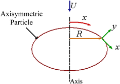
Coordinates for thin thermal boundary layer approximation
- Re :
-
Reynolds number
- Re d :
-
Reynolds numbers based on diameter
- \( Re_{\sqrt A } \) :
-
Reynolds numbers based on square root of surface area
- s :
-
Upstream distance (m) (Fig. 3)
- T :
-
Temperature (K)
- T s :
-
Body surface temperature (K)
- T ∞ :
-
Flow temperature (K)
- t :
-
Time (s)
- U :
-
External flow velocity (m/s)
- u x :
-
Velocity component in the direction of x (m/s)
- u y :
-
Velocity component in the direction of y (m/s)
- v :
-
Axis of abscissa in Fig. 2
Fig. 2 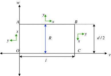
Geometric parameters of cylindrical body
- w :
-
Axis of ordinate in Fig. 2
- x :
-
Coordinate parallel to the surface of the body (Fig. 1)
- X :
-
Dimensionless x, Eq. 10
- X M :
-
Maximum value of X
- y :
-
Coordinate normal to the surface of the body (Fig. 1)
- α :
-
Thermal diffusivity (m2/s)
- ɛ :
-
Average error of curve fitting
- ζ s :
-
Surface vorticity (s−1)
- Ξ:
-
Dimensionless R, Eq. 11
- ρ :
-
Density (kg/m3)


References
Clift R, Grace GR, Weber ME (1978) Bubbles, drops and particles. Academic Press, New York
Polyanin AD, Kutepov AM, Vyazmin AV, Kazenin DA (2002) Hydrodynamics, mass and heat transfer in chemical engineering. Taylor and Francis, London
Kreith F, The CRC (2000) Handbook of thermal engineering. The mechanical engineering handbook series. CRC Press/Springer, New York
Pop I, Kumari M, Nath G (1989) Combined free and forced convection along a rotating vertical cylinder. Int J Eng Sci 27(3):193–202
Richelle E, Tasse R, Riethmuller ML (1995) Momentum and thermal boundary layer along a slender cylinder in axial flow. Int J Heat Fluid Flow 16:99–l05
Agarwala M, Chhabraa RP, Eswaranb V (2002) Laminar momentum and thermal boundary layers of power-law fluids over a slender cylinder. Chem Eng Sci 57:1331–1341
Wiberg R, Lior N (2005) Heat transfer from a cylinder in axial turbulent flows. Int J Heat Mass Transf 48:1505–1517
Sawchuk SP, Zamir M (1992) Boundary layer on a circular cylinder in axial flow. Int J Heat Fluid Flow 13(2):184–188
Bourne DE, Davies DR (1958) Heat transfer through the laminar boundary layer on a circular cylinder in axial incompressible flow. QJMAM 11(1):52–66
Seban RA, Bond R (1951) Skin -friction and heat-transfer characteristics of a laminar boundary layer on a cylinder in axial incompressible flow. J Aeronaut Sci 18:671–675
Nowak W, Stachel AA (2005) Convection heat transfer during an air flow around a cylinder at low Reynolds number regime. J Eng Phys Thermophys 78(6):1214–1221
Hoerner SF (1965) Fluid-dynamic drags (Published by the Author)
Patankar S (1987) Numerical heat transfer and fluid flow. Hemisphere, Washington, DC
Yovanovich MM (1987) Natural convection from isothermal spheroids in the conductive to laminar flow regimes. In: Proceedings of AIAA 22nd Thermophysics Conference, June 8–10, Honolulu, Hawaii
Yovanovich MM (1988) General expression for forced convection heat and mass transfer from isothermal spheroids. In: Proceedings of AIAA 26th Aerospace Science meeting, January 11–14, Reno, Nevada
Lee S, Yovanovich MM, Jafarpur K (1991) Effects of geometry and orientation on laminar natural convection from isothermal bodies. J Themophys Heat Transf 5:208–216
Jafarpur K (1992) Analytical and experimental study of laminar free convection heat transfer from isothermal convex bodies of arbitrary shape. Ph. D. thesis, University of Waterloo, Canada
Bigdely MR (1998) Conduction limit calculation using panel method. M.S thesis, Shiraz University, Shiraz, Iran
Smythe WR (1956) Charged right circular cylinder. J Appl Phys 27(8):917–920
Smythe WR (1962) Charged right circular cylinder. J Appl Phys 33(10):2966–2967
Yovanovich MM, Culham JR, Lee S (1996) Natural convection from horizontal circular and square toroids and equivalent cylinders. 96–1838 at the 31st AIAA Thermophysics Conference, June 18–20, New Orleans, LA
McAdams (1954) Heat transmission. 3rd edn. McGraw-Hill, New York
White FM (2003) Fluid mechanics. 5th edn. McGraw-Hill Series in Mechanical Engineering
Culham JR, Yovanovich MM, Teertstra P, Wang C-S, Refai-Ahmed G, Min-Tain Ra (2001) Simplified analytical models for forced convection heat transfer from cuboids of arbitrary shape. J Electron Packag 123:182–188
Author information
Authors and Affiliations
Corresponding author
Rights and permissions
About this article
Cite this article
Hadad, Y., Jafarpur, K. Laminar forced convection heat transfer from isothermal cylinders with active ends and different aspect ratios in axial air flows. Heat Mass Transfer 47, 59–68 (2011). https://doi.org/10.1007/s00231-010-0669-4
Received:
Accepted:
Published:
Issue Date:
DOI: https://doi.org/10.1007/s00231-010-0669-4