
Abstract
A multi-objective evolutionary search algorithm using a travelling salesman algorithm and genetic algorithm for flow-shop scheduling is proposed in this paper. The initial sequence is obtained by solving the TSP. The initial population of the genetic algorithm is created with the help of a neighbourhood creation scheme known as a random insertion perturbation scheme, which uses the sequence obtained from TSP. The proposed algorithm uses a weighted sum of multiple objectives as a fitness function. The weights are randomly generated for each generation to enable a multi-directional search. The performance measures considered include minimising makespan, mean flow time and machine idle time. The performance of the proposed algorithm is demonstrated by applying it to benchmark problems available in the OR-Library.
1 Introduction
Flow-shop scheduling deals with the sequencing of processing jobs, where each job is to be processed with an identical sequence of machines or stages. In a flow shop, each operation (except the first) has exactly one predecessor and each operation (except the last) has exactly one direct successor [1]. Each job requires a specific sequence of operations to be carried out for the job to be completed. The flow shop problem is a NP problem [2]. Heuristic search algorithms are more suitable in coming closer to an optimal solution at a faster rate when solving such problems. Very few researchers have tried using a genetic algorithm with multiple objectives. A multi-objective genetic algorithm for flow-shop scheduling is proposed in this paper. The objectives considered are minimisation of makespan time, minimisation of machine idle time and minimisation of mean completion time.
2 Review of flow shop literature
Rajendran and Zeigler [3] developed a heuristic procedure with the objective of minimising the makespan, where setup, processing and removal times were separable. The heuristic was evaluated by a large number of randomly generated problems.
Dipak Leha and Mukerjee [4] proposed a genetic algorithm based methodology with a view toward minimising the makespan of the schedule generated in a flow shop environment. Minimisation of makespan results in maximisation of overall resource utilisation. This algorithm is tested computationally and compared with the best existing heuristic algorithm. It yields a superior solution but the execution time is higher. Chen et al. [5] generated a genetic algorithm based heuristic for flow shop problems and compared the computational results of the heuristic with the results of existing heuristics.
Dudek et al. [6] reviewed flow shop sequencing research since 1954 that was devoted to the static deterministic case in which n jobs are to be processed through a shop in which the processing times at each stage are fixed. They also comment on NP completeness, selection criteria for optimisation and the lack of application of this work in industry. Widmer and Hertz [7] proposed a new heuristic method for solving m-machine, n-job flow-shop scheduling problems. It is composed of two phases: the first phase finds an initial sequence using an analogy with the travelling salesman problem and the second improves the solution using a tabu search technique.
Chen et al. [8] proposed a GA-based heuristic for continuous flow shop problems with total flow time as the criteria. The effects of several crucial factors of GA on the performance of the heuristic for the problems are explored. Murata et al. [9] applies GA to a flow-shop scheduling problem and examines the hybridisation of the GA with other search algorithms.
Taillard [10] proposed 260 randomly generated scheduling problems, the size of which is greater than that of the rare examples published and which correspond to real dimensions of industrial problems.
Rajendran [11] developed a new heuristic for a flow-shop and flow-line based manufacturing cell with the bi-criteria of minimising makespan and total flow time of jobs. Santos et al. [12] investigated scheduling procedures that seek to minimise the makespan in a static flow shop within a multiple processor scheduling environment. The development is performed to achieve good initial sequence for multiple processors.
Sharada Priyadarshini and Rajendran [13] consider the presence of different buffer space requirements for jobs and constraints on buffer capacity between machines for the problem of scheduling in a permutation flow shop. They proposed the generalised formulation of recursive equations for timetabling of jobs in a buffer constrained flow shop.
Fischera et al. [14] considered genetic algorithm efficiency in solving a pure flow-shop scheduling problem. Different formulations of the crossover operator ad setting of control parameters were investigated in order to obtain enhanced performances in the determination of minimum makespan schedules. Mulkens [15] stated that new iterative techniques like GA have proven to be efficient. They showed that those techniques may even be better than the Johnson algorithm for 2- and 3-machine cases. A comparison is also made with multi-machine flow shop CDS and NEH heuristics.
Lee et al. [16] considered GA for general machine scheduling problems and traditional job shop scheduling, flow-shop scheduling and open shop scheduling. Zegordi et al. [17] proposed a simulated annealing algorithm for the flow-shop scheduling problem. From the computational results, they showed that the solutions obtained by the proposed method were superior to those of traditional heuristics.
Wen et al. [18] proposed an algorithm using tabu search and reported that the results obtained were superior compared to other heuristic methods. Taillard et al. [19] performed a comparative study of the best heuristic methods to solve the flow shop sequencing problem and also proposed a parallel tabu search algorithm. They indicated that tabu search heuristic performs better.
Ponnambalam et al. [20] performed an extensive evaluation of constructive and improvement flow-shop scheduling heuristics and proposed a GA-based improvement heuristic. They reported that among the constructive heuristics, the NEH heuristic performs well and that a GA-based heuristic performs much better among all of these, including the proposed GA for the makespan objective.
3 State of the art
As the flow shop problems fall in the area of NP hard, complete enumerative techniques must be used to solve these problems. As problem size increases, this approach is not computationally practical. For this reason, researchers have constantly focused on developing heuristics for hard problems. Most of the existing heuristics are for the m-machine, n-job flow shop problem with makespan as the criterion.
Only very few researchers applied hybrid multi-objective evolutionary search algorithms to flow shop problems. There is a scope for developing a hybrid search algorithm for flow-shop scheduling problems. In this paper, an attempt has been made to develop a TSP-GA multi-objective evolutionary search algorithm for flow-shop scheduling problem with the objectives of minimisation of makespan time, minimisation of machine idle time and minimisation of mean completion time. Twenty one benchmark problems that are available in the OR-library are considered for evaluation of the proposed algorithm and the results are reported.
4 The multi-objective genetic algorithm
The algorithm starts off with a population which comprises a number of chromosomes. Each chromosome has an evaluation criterion based on the objective function. Since GA is used for maximisation problems, a minimisation problem can be suitably converted into a maximisation problem using a fitness function. The fitness function used in this paper is,
where x is the objective function to be minimised. The term F represents the fitness of the chromosome under consideration. Each chromosome is thus characterised by a fitness. The genetic algorithm consists of three operators: the selection operator, the crossover operator and the mutation operator. During selection, chromosomes with better fitness value stand a better chance of being selected in the mating pool. Probabilities for crossover and mutation are fixed to a certain value depending upon the nature of the problem. If the conditions specified for crossover and mutation are met the chromosomes produce new offspring, which replace their parents in the population. The new offspring shall be repeated in the next generation if their fitness is superior to those of the others in the population. The process is repeated to a number of generations. The various GA parameters suggested by Ponnambalam et al. [20] used in this paper are given in Table 1. The various parameters used in the MOGA are explained in this section. The general schema of the MOGA is given below.
4.1 General schema
Input process time matrix
Calculate the distance matrix
Identify the seed sequence
Generate the initial population using RIPS
do
{
evaluation of population
Selection
Crossover
Mutation
} until(termination condition)
4.2 Generation of seed sequence using TSP
Widmer and Hertz [7] proposed a procedure that creates a distance matrix using the processing time matrix (Table 2). They also developed a TSP procedure that utilises insertion logic to obtain the sequence of jobs. The seed sequence obtained is used to derive the schedule. The input is an n-job, m-machine matrix of processing times that yields the distance matrix. The equation used to get the distance matrix is given below:
where
- t a1 =:
-
time spent by job a on machine 1,
- t bm =:
-
time spent by job b on machine m,
- t ak =:
-
time spent by job a on machine k, and
- t b,k−1 =:
-
time spent by job b on machine k−1
Having formed the distance matrix, the element having the least value is selected. The diagonal elements are not considered, as the jobs are the same. Having selected the jobs, an insertion heuristic is used until the final sequence is generated. The function of the procedure for obtaining the seed sequence is explained in the next section.
4.2.1 Generation of distance matrix
The following example of five jobs to be processed on three machines, shown in Table 1, is used to illustrate the generation of the seed sequence.
The distance matrix for the example problem is given in Table 3. The calculation of distance for element d 12 is explained below. Similarly, the other elements of the distance matrix are calculated.
Substituting the values in the equation the d 12=3+1+3=7.
4.2.2 Generation of seed sequence
The insertion method proposed by Widmer and Hertz [7] is used to obtain the seed sequence. The insertion method is explained below:
- Step 1::
-
Find a and b such that d ab =min ij d ij
Path=a→b
- Step 2::
-
while all jobs are not sequenced do
choose an unsequenced job (randomly)
introduce it so that it causes the minimal increase of the total
length of the path
end while
The formation of seed sequence for the example problem is explained in this section. The least element of the distance matrix, i.e. 4, is selected. The corresponding jobs to be selected are 5 and 1. A random third job is inserted in each of the three spaces shown at a time.
_5_1_
The randomly selected job is assumed to be 2. This insertion gives rise to three sequences, 251, 521 and 512.
Each sequence is evaluated using the distance matrix as follows:
- For sequence 2 5 1:
-
distance=d 25 +d 51 =9+4=13
- For sequence 5 2 1:
-
distance=d 52 +d 21 =5+6=11
- For sequence 5 1 2:
-
distance=d 51 +d 12 =4+7=11
The sequence with the least of the three values is selected. In this case any one of 521 and 512 can be selected. The procedure is repeated until the final sequence of 5 jobs is obtained. Thus an analogy of the TSP is used to obtain a seed sequence for flow-shop scheduling.
4.3 Creation of initial population
A neighbourhood creation scheme, random insertion perturbation scheme (RIPS) proposed by Parthasarathy and Rajendran [21] is used to generate the initial population. The seed used for this scheme is the one generated using the TSP logic proposed by Widmer and Hertz [7]. The idea is to start off with a population that has better fitness values than a population that is generated randomly. This is done because with the better population, the GA may come up with a better solution (a better sequence) than that of a GA that uses a randomly generated population. The RIPS method is illustrated with an example. In the RIPS technique, the jobs at the beginning and at the end need only one random number as they can shift in only one direction while the others need two random numbers—one for a shift to the right and one for a shift to the left. In this manner (2n−2) sequences are generated for an n job problem. The functioning of the RIPS is explained with an example. Assume the seed sequence is 5-2-4-1-3. The neighbourhoods created are given in Table 4 and this is the initial population for the MOGA.
4.4 Evaluation of chromosomes
The chromosomes are evaluated using the objective functions considered in this paper. The three objective functions need to be combined into a single objective function f i . For this purpose three random weights w 1, w 2, and w 3 are generated, such that, w 1+w 2+w 3=1. For each chromosome, the combined objective function is the minimisation of x given by:
Since GA is used for maximisation problems the minimisation problem is converted into a maximisation problem using the following fitness function:
Where, F is the fitness of a sequence or chromosome.
The objective function values and the fitness function values are given in Table 5.
4.5 The selection operator
The selection operator is also called the reproduction operator. This operator produces the mating pool consisting of chromosomes with good fitness values. The chromosomes are compared on the basis of their fitness values. There are various selection operators available that can be used to form the mating pool. The tournament selection is used in this paper.
The tournament selection operator randomly shuffles the population and compares, in order, two chromosomes at a time. The better chromosome makes it to the mating pool. The shuffling is done twice to maintain the population size as constant. After performing the selection, the mating pool obtained is given in Table 6.
It is worthwhile here to note that the chromosomes with better fitness values may get repeated. For example, the mating pool has the chromosome 25413 twice and it happens to be the fittest chromosome of the population. The same is true for the second fittest chromosome 54213.
4.6 The crossover operator
The matting pool is ready for crossover. A partially mapped crossover operator is used in this paper. Details about the perturbation of the population after crossover are given in Table 7. The probability of crossover is assumed to be 0.6.
4.7 The mutation operator
The reciprocal exchange mutation has a probability of mutation of 0.05 in this paper. The details of the mutation operation are explained in Table 8.
This completes one generation and the algorithm is designed for 250 generations. The best solution is identified after 250 generations.
5 Results and discussion
Twenty-one benchmark problems available in OR-Library (http://www.ms.ic.ac.uk) were solved using the proposed MOGA. The results are given in Table 9. The best chromosomes in all 250 generations are stored. Since the fitness values continue to vary, selecting the right chromosome or the optimal sequence based solely on the fitness might not give the right sequence. A sequence may be repeated due to its superior. Repetition must be taken into account. The following heuristics are followed to select the best chromosome for each problem. The heuristics are mainly based on two factors: fitness values and repetition of the fitter sequences.
- Step 1:
-
From the 250 solutions of fitness, the ten best values are selected.
- Step 2:
-
The sequences corresponding to these ten values are noted.
- Step 3:
-
Any repetition of a particular sequence amongst these ten sequences is noted.
- Step 4:
-
The sequence that gets repeated most often is selected. In the case of two or more sequences that have the same number of repetitions, the sequence with better fitness values is selected.
- Step 5:
-
If no sequence is repeated, the sequence with the best fitness value is selected.
5.1 Discussion
An observation of the results and methodology provides the following points that merit discussion.
-
1.
Any system is judged based on the time taken for its completion and the utilisation of its resources. This forms the basis for the selection of a multi-objective criterion in this paper. The values of makespan, mean flow time and machine idle time are optimised to strike a balance between these values and to obtain the best possible sequence for a given problem.
-
2.
Genetic algorithms are mainly applied to single-objective optimisation problems. When a single-objective genetic algorithm is applied to a multi-objective optimisation problem, multiple objective functions should be combined to form a scalar fitness function. If a constant weight is assigned to each of the multiple objective functions for combining them, the direction of search in the genetic algorithm is constant as shown in Fig. 1. A scalar fitness function, which uses randomly generated weighs to sum of objective functions, is used in this paper. The weights attached to the multiple objectives are not constant but randomly specified in each selection from Murata et al. [9]. In this paper a similar procedure for calculation of the fitness of each chromosome is adopted. Hence, the direction of search is not constant as shown in Fig. 2.
Fig. 1 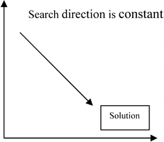
Search direction with constant weights
Fig. 2 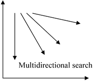
Multidirectional search with random weights
-
3.
The proposed MOGA starts with the initial solution generated using TSP. That enables a faster search to reach the best solution. It is often found that the best solution obtained is very close to the initial solution or that it has been obtained in the early stages of the genetic algorithm. This indicates the strength of the initial solution obtained from TSP. A direct advantage of this is reduction in computation time.


References
Baker KR (1974) Introduction to sequencing and scheduling. Wiley, New York
Pinedo M (1995) Scheduling: theory, algorithms, and systems. Prentice Hall, New Jersey
Rajendran C, Zeigler H (1997) Heuristics for scheduling in a flow shop with set-up, processing and removal times separated. Product Plan Contr 8:568–576
Dipak Leha MIIE, Mukerjee SP (1998) Flow-shop scheduling using genetic algorithms for minimizing makespan. Indian Inst Ind Eng J 27:4–8
Chen C-L, Vempati VS, Aljaber N (1995) Theory and methodology—an application of genetic algorithms for flow shop problems. Eur J Oper Res 80:389–396, 1995
Dudek RA, Panwalkar SS, Smith ML (1992) The lessons of flow-shop scheduling research. Oper Res 40:7–13
Widmer M, Hertz A (1989) A new heuristic method for the flow shop sequencing problem. Euro J Oper Res 41:186–193
Chen C-L, Neppalli RV, Aljaber N (1996) Genetic algorithms applied to the continuous flow shop problem. Comput Ind Eng 30:919–929
Murata T, Ishibuchi H, Tanaka H (1996) Algorithms for flow-shop scheduling problems. Comput Ind Eng 30:1061–1701
Taillard E (1993) Benchmarks for basic scheduling problems. Eur J Oper Res 64:278–285
Rajendran C (1994) A heuristic for scheduling on flow shop and flow line based manufacturing cell with multi criteria. Int J Prod Res 32:2541–2558
Santos DL, Hunsucker JL, Deal DE (1996) An evaluation of sequencing heuristics in flow shops with multiple processors. Comput Ind Eng 30(4):681–692
Sharada Priyadarshini B, Rajendran C (1996) Formulation and heuristics for scheduling in a buffer constrained flow shop and flow line based manufacturing cell with different buffer space requirements for jobs: part 1. Int J Prod Res 34:3465–3483
Fischera S, Grasso V, Lombardo A, Lo Valvo A, Lo Valvo E (1995) Genetic algorithms efficiency in flow-shop scheduling. In: Applications of Artificial Intelligence in Engineering, pp 261–270
Mulkens H (1994) Revisiting the Johnson algorithm for flow-shop scheduling with genetic algorithms. IFIP Trans B: Comput App Tech 15:69–80
Lee K, Yamakawa, Takeshi L, Keon-Myung (1998) Genetic algorithm for general machine scheduling problems. In: proceedings of international conference on knowledge-based intelligent electronic systems 2, pp 60–66
Zegordi SH, Itoh K, EnkawaT (1995) Minimizing makespan for flow-shop scheduling by combining simulated annealing with sequencing knowledge. Eur J Oper Res 85:515–531
Wen, Pyng U, Yeh, Ching I (1997) Tabu search methods for the flow shop sequencing problem. J Chinese Inst Eng Trans 20:465–470
Taillard E (1990) Some efficient heuristic methods for the flow shop sequencing problem. Eur J Oper Res 47:65–74
Ponnambalam SG, Aravindan P, Chandrasekaran S (2001) Constructive and improvement flow-shop scheduling heuristics: an extensive evaluation. Prod Plan Contr 12(4):335–344
Parthasarathy S, Rajendran C (1997) An experimental evaluation of heuristics for scheduling in a real life flow shop with sequence-dependent set up time of jobs. Int J Prod Econ 49:255–263
Author information
Authors and Affiliations
Corresponding author
Rights and permissions
About this article
Cite this article
Ponnambalam, S.G., Jagannathan, H., Kataria, M. et al. A TSP-GA multi-objective algorithm for flow-shop scheduling. Int J Adv Manuf Technol 23, 909–915 (2004). https://doi.org/10.1007/s00170-003-1731-x
Received:
Accepted:
Published:
Issue Date:
DOI: https://doi.org/10.1007/s00170-003-1731-x