
Abstract
The evolution laws of LURR (Loading–Unloading Response Ratio) before strong earthquakes, especially the peak point of LURR, are described in this paper. The results of four methods (experimental, numerical simulation, seismic data analysis and with damage mechanics analysis) lead to a consistent conclusion—the evolution laws of LURR before strong earthquakes are that, at the early stage of the seismic cycle, LURR will fluctuate around 1 and in the late stage, it rises swiftly and to its peak point. At some time after this peak point, a catastrophic event or events occur. These do not occur at the peak point, but lag behind. The lag time which is denoted by T 2 depends on the magnitude M of the upcoming earthquake among other factors. In order to consider the influence of geophysical parameters in a specific region such as \( \dot{\gamma }, \) E a and J (t), where \( \dot{\gamma } \) is the shear strain rate of tectonic loading in situ, E a is the sum of radiated energy of all earthquake occurring in a specific region measured during a long time duration (110 years in this paper) divided by the area of the region and the time duration, and J (t) is a parameter denoting the LURR anomaly area weighted with Y (the value of LURR) and represents the expanse and degree of the seismogenic zone. The dimensional analysis method has been used to reveal the relation between M, T 2 and other parameters in situ for more reliable earthquake prediction.
1 Introduction
Earthquakes are one of the most complicated natural phenomena. But from the view point of mechanics, the physical essence of earthquake is quite clear that it is just an abrupt shear rupture and sliding in a seismic source region accompanied by a sudden release of strain energy. Consequently, the seismogenic process should be a damage process of the focal media leading to the abrupt shear rupture. In other words, the seismogenic process is one of damage evolution which finally results in the occurrence of an earthquake. The basic idea of Load/Unload Response Ratio (LURR) consists of depicting the damage of the seismogenic zone with the LURR measure, and then using this physical parameter as a basis to predict earthquakes. It has been about 30 years since LURR has been put forward (Yin, 1987, 1993; Yin and Yin, 1991; Yin et al., 1994, 2006). Since then, many basic problems have been studied, such as the means and criteria of loading and unloading of a crustal block with spatial extent reaching up to around 1000 km, the choice of responses to use in calculating LURR, retrospective studies of LURR for earthquake cases and the practice of earthquake prediction. In particular, the prediction of the location of the upcoming strong earthquakes has proven to be successful to a considerable extent. Namely,—95% earthquakes with magnitude ≥5 have occurred within the LURR anomaly region during 2004–2007 on the Chinese mainland (Institute of Earthquake Science 2008). Many scientists who do not belong to our team have also conducted research on different kinds of problems with or related to LURR and have published over one hundred papers (Trotta and Tullis, 2006; Xu and Huang, 1995a, b; Xia, et al., 2002; Yin, 2005; Yu, et al. 2006; Zhang et al., 2006b, etc. incomplete list due to space limitation).
2 Peak Point of LURR and Its Significance
In recent years, we have worked out the evolution laws of LURR before strong earthquakes by many different means. Figure 1a through 1d show: (a) Experimental data: the evolution of LURR as a function of time in an acoustic emission experiment (Yu, et al., 2003; Yin, et al., 2004; Zhang et al. 2006a); (b) Observed earthquake data: evolution of LURR before the October 17, 1989 Loma Prieta earthquake (Yin, 1993; Yin, et al., 1993, 1995, 2000, 2006); (c) Simulated damage evolution of a non-uniform brittle medium: evolution of LURR with time by numerical simulation (Wang, et al., 2000; Mora, et al. 2002; Liang, et al., 1998; Zhang, 2009); (d) The damage evolution of a non-uniform brittle medium simulated with the Lyakhovsky model and the analytic result of LURR as a function of time (Lyakhovsky, et al. 1997, 2001; Zhang, 2009). The arrows indicate catastrophic events (earthquakes or catastrophic failure of a laboratory, numerical or theoretical specimen). The results of the four methods are consistent and all result in the same conclusion that in the early stages of the seismic cycle, LURR fluctuates around 1 and then it rises swiftly to its peak point (abbreviated pp). Catastrophic events do not occur at this peak point, but after it. Namely, the catastrophic events lag behind the peak point. This result is similar to what has been observed for results obtained based on the Critical Point Hypothesis for earthquakes where once the theoretical critical point is reached based on curve fitting (e.g. Bowman, et al., 1998; Yin, et al., 2002, Wang, et al., 2004), the earthquake fault system is “primed” to enable a large runaway earthquake, but the large event occurs at some time later than the predicted critical point time or after stress correlations have built up within the system (Mora and Place, 2002).

The evolution of LURR before strong earthquake or catastrophic rupture in experiment
In this paper, we aim to improve understanding of the predicted magnitude and lag time of the large earthquake predicted by the LURR method, and hence, make advances in the potential reliability and accuracy of LURR for short to intermediate term earthquake forecasting. The lag time is denoted T 2, the time from the beginning of the LURR anomaly to the peak point is denoted by T 1, and the total abnormal time is denoted by T,
According to research (Zhang, 2006)
where M denotes the earthquake magnitude and T scales with month. Table 1 (Zhang, 2006) shows that while T 2 is much shorter than the seismic cycle, it is still quite a long time, e.g. T 2 is about 14 months for an earthquake with magnitude 6, T 2 is more than 2 years for an earthquake with magnitude 7, and T 2 could be 36 months (28 ± 8) for earthquakes of magnitude 8, namely as long as 3 years. This means that the “big” earthquake does not occur at the peak point (where LURR reaches its biggest value), but on the of order many months to a few years later after the LURR value has decreased from its peak value, sometimes down to a value even less than 1. This was exactly the situation in the case of the 2008 Wenchuan earthquake. Although we discovered a long time duration LURR anomaly in this area (Yin, et al., 2006), we predicted that a strong earthquake would likely occur in this area during August 2006 to March 2008. However, at the end of 2007 it had still not occurred. In China, at the end of each year we are asked to provide a report to predict the earthquake tendency for the next year. In this report, we did not continue to insist on this prediction since the expected event did not occur by the end of 2007 even though the LURR anomaly existed for a long time (several years) and our initial time window for the predicted event was up to March 2008. Rather, we thought the prediction made in 2006 was likely a false one.
The above results (Eqs. 1–3; Table 1) have great importance on the practice of earthquake prediction since these equations provide a method for predicting the approximate occurrence time and its accuracy quantitatively (to a scale of months) if T pp (the time of the peak point) can be accurately calculated. Above all, based on the consistency of the LURR patterns in the laboratory, numerical simulations and theoretical analysis of damage mechanics with LURR patterns in seismic data, the variation of LURR could depict clearly the seismogenic process, and with equations such as 1 through 3, it may offer further ideas and methods for developing more reliable and quantitative earthquake prediction methods.
3 Improving the Prediction of Magnitude M and T 2—Integrating LURR with the Dimensional Analysis Method
If the time of peak point has been determined, then T 2 can be calculated from formula (3) and hence, the occurrence time and error bars of the future earthquake could be predicted (Zhang, 2006). But it has been discovered that T 2 is not only a function of M, but also depends on other physical parameters in situ. For example, the cases of the Xinjiang Uygur Autonomous Region usually have a much shorter T 2 than the results calculated from formula (3) (personal communication with professor Wang Haitao who worked at the Seismological Bureau of Xinjiang Uygur Autonomous Region), so we use the dimensional analysis method (Sedov, 1959) to study the problem. We use non-dimensional quantities (π) instead of dimensional quantities to reveal the relation between M, T 2 and other parameters. It is postulated that magnitude M s (or its equivalent parameter E s, according to Gutenberg formula E s = 4.8 + log 1.5 M) and T 2 could be separately related to the parameters: J, E a and\( \dot{\gamma }. \)
Where
-
(a)
A measure of LURR anomaly, J (t)
$$ J_{(t)} = \iint\limits_{R} {Ydxdy} $$(4)R{Y ≥ 1}, R denoted the region of LURR anomaly region.
J (t) is defined as in formula (4) which is used to denote the LURR anomaly area weighted with Y (the value of LURR) and represents the expanse and degree of the LURR anomaly region (seismogenic zone) during a specific time window [from (t−t w) to t]. In fact, J (t) = Y a A, where A is the area of the LURR anomaly region and Y a is the average value of LURR for A. J pp means the value of J at peak point (pp) or the maximum of J. In order to calculate the value of J pp, the spatial scans of LURR for the Chinese mainland should first be conducted for a series of times (e.g. Fig. 2). Subsequently, J (t) is calculated according to Eq. 4. For example, Fig. 3 shows us the curve of J (t) for the Kaifeng region in the Henan province in east China. The P tt was January 2011, at that time J (t) reached its maximum value J pp (2.67 × 10⁵ km2).
Fig. 2 
The map of LURR scanning results in Chinese mainland in recent years
Fig. 3 
The curve of J (t) for Kaifengin region in Henan province in east China. The red vertical lines denote the significant earthquakes in the same region. J pp = 2.67 × 10⁵ km2 at T pp (January 2011)
-
(b)
Radiated seismic energy, Ea: E a is defined as the sum of radiated energy of all earthquakes occurring in a specific region per year and per area measured during a long enough time duration which mirrors its average intensity of seismicity in a special region. In this paper we use the catalog from 1900 to 2009 of the Chinese mainland. That means the duration is 110 years. The distribution of E a in the Chinese mainland is shown in Fig. 4 in which the energy has transformed to magnitude M (in this paper magnitude M always means M s) according to the Gutenberg formula and shown with the color bar at the right of the Figure.
Fig. 4 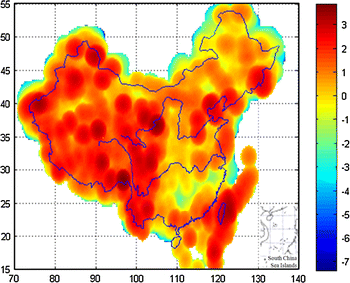
The distribution of E a in Chinese mainland
-
(c)
Strain rate, \( \dot{\gamma }: \) \( \dot{\gamma } \) is the shear strain rate in situ. The distribution of \( \dot{\gamma } \) in the Chinese mainland can be obtained from the GPS measured results (Shen, et al., 2003; Gu, et al., 2001; Li et al. 2004).


There are 5 parameters involved (E s, T 2, E a, \( \dot{\gamma } \) and J pp) and 3 fundamental units (length, time and mass) in our problem. According to π-theorem (Buckingham, 1914), two non-dimensional quantities (π1 and π2) can be formed as below:
and
Fitting the data of about 50 earthquake cases on the Chinese mainland (magnitude from 4.7 to 8.1 and in recent years), we obtained that the curves and functions of π 1 versus M s (magnitude) and π3 versus M s (Figs. 5, 6). According to the Gutenberg formula E s = 4.8 + log 1.5 M and then it is obtained:

The curve of π 1 versus m (magnitude)

The curve of π2 versus m
and
when the J pp , E a and \( \dot{\gamma } \) for a specific region have been obtained, the magnitude M s of the upcoming earthquake can now predicted from expression (8) and then the lag time T 2 can be obtained from expression (9). As an example of the application of this methodology, we researched the case of the Zhoukou earthquake. It is found that an LURR anomaly region appeared in the Kaifeng region (in the Henan province in east China) (Fig. 7). According to the LURR spatial scanning of LURR for different time windows, J (t) and then J pp, and T pp were obtained (Fig. 3) (T pp = January 2011 and J pp = 2.67 × 10⁵ km2). Hence, according to Eqs. 8 and 9, the magnitude of the upcoming earthquake is estimated to be M s = 4.4 ± 0.5, and the time lag from T pp of the event is approximately T 2 = 11 ± 2 months (Korn, 2000) An earthquake with magnitude 4.7 occurred on October 24, 2010, in the town of Zhoukou (the epicenter is 34.1 N; 114.6). The epicenter (34.1 N°; 114.6°E) falls inside the seismogenic zone in Fig. 7 and its magnitude and occurrence time both fall within the predicted ranges. Though an earthquake with magnitude of 4.7 is not strong, this event was the biggest one in that region during the last half-century.

The seismogenic zone of Zhoukou earthquake
Another case is in the expansive southwestern region (including Tibet, Qinghai and Yunnan). We have found a LURR anomaly region with a very large scale for many years in this region. Using the above method we roughly estimate that the magnitude of the future earthquake will be above M8 even M9, and its J (t) has not reached maximum yet, so we are not able to predict its lag time and hence occurrence time at present.
4 Conclusions and Discussions
Since the proposal of LURR, more than two decades have elapsed (Yin et al., 2006). Many achievements have been made in LURR theory and application during this long time including successful intermediate-term predictions and improved understanding of its physical mechanism and limitations, but there still exist many problems and also room for improvement, e.g. an understanding of the evolution law of LURR after the peak point may be useful for the application of the LURR method to short-term earthquake prediction.
As to the application of the dimensional method, the crucial problems are how to obtain/choose the parameters in situ. For example, the shear strain rate \( \dot{\gamma } \) of a specific region might change with time and if so, we would need to obtain some additional data to resolve this variation.
This paper is just a primary study on the application of the dimensional method to earthquake prediction. We need to do more works such as more cases study retrospectively and on prediction practice.
References
Bowman, D. D., Ouillen, G., Sammis, C. G., Sornette, A., and Sornette, D. (1998) An observational test of the critical earthquake concept, J. Geophys. Res. 103, 24, 359–24, 372
Buckingham, E., (1914) On physically Similar Systems: Illustrations of the Use of Dimensional Analysis, Physical Review, 4, 345–376.
Gu G., Shen X., Wang M., Zheng G., Fang Y. and Li P., (2001), General characteristics of the recent horizontal crustal movement in Chinese mainland, ACTA SEISMOLOGICA S IN ICA, 23, No. 4, 362–369.
Institute of Earthquake Science, (2008) Final Report, in book ≪Research on prediction of the strong earthquake tendency in Chinese Mainland for 2009, (edited by Institute of Earthquake Science, China Seismological Bureau,)≫, PP 1–93, Seismological Press, Beijing, (in Chinese).
Korn, T.M., (2000) Mathematical Handbook, §19.2–4, DOVER PUBN INC.
Li Y. X., Li Z., Zhang J. H., et al., (2004) Horizontal strain field in the Chinese mainland and its surrounding areas. Chinese J. Geophys. (in Chinese), 47 (2), 222–231.
Liang, N. G., Liu, H. Q. and Wang, T. C., (1998), A meso elastoplastic constitutive model for polycrystalline metals based on equivalent slip systems with latent hardening. Science in China, Ser. A. 41, 887–896.
Lyakhovsky V., Ben-Zion Y., and Acnon A., (1997), Distributed Damage, Faulting. And Friction, J. Geophys. Res. 102, 27, 635–627, 649.
Lyakhovsky V., Ben-Zion Y., and Agnon A., (2001) Earthquake Cycle, Fault Zones, And Seismicity Patterns In A Rheologically Layered Lithosphere, J. Geophys. Res., 106, 4103–4120.
Mora, P., Wang, Y., Yin, C., Place, D. and Yin, X.C., (2002) Simulation of Load-unload Response Ratio and Critical Sensitivity in the Lattice Solid Model, Pure Appl. Geophys., 159, 2525-P.
Mora, P. and Place, D., (2002) Stress correlation function evolution in lattice solid elasto-dynamic models of shear and fracture zones and earthquake prediction, Pure Appl. Geophys., 159, 2413–2427.
Sedov, L.I., (1959) Similarity and Dimensional Methods in Mechanics, NFOSEARCH LTD. London.
Shen Z.K., Wang M., Gan W.J., and Zhang Z.S., (2003), Contemporary Tectonic Strain Rate Field Of Chinese Continent And Its Geodynamic Implications, Earth Science Frontiers, 10 suppl., 93–100.
Trotta J.E., and Tullis T.E., (2006) An independent assessment of the Load/Unload Response Ratio (LURR) proposed method of earthquake prediction, Pure and Applied Geophysics, 163(11–12), 2375–2388.
Xia M.F., Wei Y.J., Ke F.J., and Bai Y.L., (2002), Critical sensitivity and trans-scale fluctuations in catastrophe rupture, Pure Appl. Geophys., 159(10): 2491–2509.
Xu Q., and Huang R.Q., (1995b), Investigation on precursor of slope instability in term of LURR, Chinese Journal of Geological disasters, Vol. 6, No. 2.
Xu Q., and Huang R.Q., (1995b), A theoretical Study of the slope instability using the Theory of Load/Unload Response Ratio (LURR), The Chinese Journal of Geological Hazard and Control, Vol. 6, 22–31.
Wang Y.C., Yin X.C., Ke F.J., Xia M.F., and Peng K.Y., (2000), Numerical Simulation of Rock Failure and Earthquake Process on Meso-scopic Scale, Pure Appl. Geophys., 157, 1905–1928.
Wang Y.C., Yin C., Mora P., Yin X.-C., and Peng K-Y. (2004) Spatio-temporal scanning and statistical test of the accelerating moment release (AMR) model using Australian earthquake data, Pure Appl. Geophys., 161, 2281–2293.
Yin C, (2005), Exploring the Underlying Mechanism of Load/Unload Response Ratio (LURR) Theory and Its Application to Earthquake Prediction, PhD Thesis of The University of Queensland, Australia.
Yin X.C., (1987), A New Approach to Earthquake Prediction, Earthquake Research in China, 3, 1–7 (in Chinese with English abstract).
Yin X.C., and Yin C. (1991), The Precursor of Instability for Nonlinear System and Its Application to Earthquake Prediction, Science in China, 34, 977–986.
Yin X.C. (1993), A New Approach to Earthquake Prediction, Russia’s “Nature”, 1, 21–27 (in Russian).
Yin X.C., Yin C and Chen X.Z. (1994), The Precursor of Instability for Nonlinear System and Its Application to Earthquake Prediction—the Load-Unload Response Ratio Theory, In “Non-linear Dynamics and Predictability of Geophysical Phenomena”, (eds. Newman, W.I., Gabrelov, A, and Turcotte, D.L.), Geophysical Monograph. 83, IUGG Volume 18, 55–60.
Yin X.C., Chen X.Z., Song Z.P., and Yin C., (1995), A New Approach to Earthquake Prediction: The Load/Unload Response Ratio (LURR) Theory, Pure Appl. Geophys, 145, 701–715.
Yin X.C., Wang Y.C., Peng K.Y., Bai Y.L., Wang H.T., and Yin X.F., (2000), Development of a New Approach to Earthquake Prediction—Load/unload Response Ratio (LURR) Theory, Pure Appl. Geophys., 157, 2365–2383.
Yin X.C., Mora P., Peng K.Y., Wang Y.C., and Weatherly D., (2002), Load-unload Response Ratio and Accelerating Moment/Energy Release, Critical Region Scaling and Earthquake Prediction, Pure Appl. Geophys., 159, 2511–2524.
Yin X.C., Yu H.Z., Kukshenko V., Xu Z.Y., Wu Z.S., Li M., Peng K.Y., Elizarov S., and Li Q., (2004), Load-Unload Response ratio (LURR), Accelerating Energy release (AER) and State Vector evolution as precursors to failure of rock specimens, Pure Appl. Geophys, 161, No.11–12, 2405–2416.
Yin X.C., Zhang L.P., Zhang H.H., Yin C., Wang Y.C., Zhang Y.X., Peng K.Y., Wang H.T., Song Z.P., Yu H.Z., and Zhuang J.C., (2006), LURR’s Twenty Years and Its Perspective, Pure and Applied Geophysics, 163(11–12), 2317–2341.
Yu H.Z., Yin X.C.,, Liang N.G., Xia M.F., Li M., Xu Z.Y., Peng K.Y., Kukshenko V., Wu Z.S., Li Q. and Elizarov S., (2003), Experimental Research on the Load/Unload Response Ratio (LURR) theory, Earthquake research in China, Vol. 17, No. 3, 227–235.
Yu H.Z., Shen Z.K., Wan Y.G., and Zhu Q.Y., (2006), Increasing critical sensitivity of the Load/Unload Response Ratio before large earthquakes with identified stress accumulation pattern, Tectonophysics, 428, 87–94.
Zhang H.H., Yin X. C., Liang N.G., Yu H. Z., Li S.Y., Wang Y.C., Yin C., Kukshenko V., Tomiline N., Elizarov S., (2006), Acoustic Emission Experiments of Rock Failure under Load Simulating the Hypocenter Condition, Pure and Applied Geophysics, 163(11–12), 2389–2406.
Zhang, H.H., (2006), Prediction of Catastrophic failure in Heterogeneous Brittle Media—Study and practice of Load/Unload Response Ratio (LURR), PhD Thesis of The Graduate School of the Chinese Academy of Sciences (in Chinese).
Zhang L.P., (2009), Study on Damage Evolution of Heterogeneous Brittle Media in Seismogenic Conditions and Earthquake Prediction, PhD Thesis of The Graduate School of the Chinese Academy of Sciences (in Chinese).
Zhang W.J., Chen Y.M., and Zhan L.T., (2006), Loading/Unloading response ratio (LURR) theory applied in predicting deep-seated landslides triggering, Engineering Geology, 82, 234–240.
Acknowledgments
This research was funded by the National Natural Sciences Foundation of China (Grant No. 19732060 and 40004002) and Informalization Construction Project of Chinese Academy of Sciences during the 11th Five-Year Plan Period (No. INFO-115-B01). The earthquake catalog used in this paper is provided by CENC (China Earthquake Networks Center), Chinese Earthquake Administration. The calculations in the paper was conducted partly in Supercomputing Center of Computer Network information Center, Chinese Academy of Sciences (CAS).
Author information
Authors and Affiliations
Corresponding author
Rights and permissions
About this article
Cite this article
Yin, Xc., Liu, Y., Mora, P. et al. New Progress in LURR-Integrating with the Dimensional Method. Pure Appl. Geophys. 170, 229–236 (2013). https://doi.org/10.1007/s00024-012-0453-0
Received:
Revised:
Accepted:
Published:
Issue Date:
DOI: https://doi.org/10.1007/s00024-012-0453-0