Computing with Formulas

Abstract

Our first examples on computer programming involve programs that evaluate mathematical formulas. You will learn how to write and run a Python program, how to work with variables, how to compute with mathematical functions such as e^x and $\sin x$, and how to use Python for interactive calculations.

Our first examples on computer programming involve programs that evaluate mathematical formulas. You will learn how to write and run a Python program, how to work with variables, how to compute with mathematical functions such as e^x and $\sin x$, and how to use Python for interactive calculations.

We assume that you are somewhat familiar with computers so that you know what files and folders are (another frequent word for folder is directory), how you move between folders, how you change file and folder names, and how you write text and save it in a file.

All the program examples associated with this chapter can be downloaded as a tarfile or zipfile from the web page http://hplgit.github.com/scipro-primer. I strongly recommend you to visit this page, download and pack out the files. The examples are organized in a folder tree with src as root. Each subfolder corresponds to a particular chapter. For example, the subfolder formulas contains the program examples associated with this first chapter. The relevant subfolder name is listed at the beginning of every chapter.

The folder structure with example programs can also be directly accessed in a GitHub repository¹ on the web. You can click on the formulas folder to see all the examples from the present chapter. Clicking on a filename shows a nicely typeset version of the file. The file can be downloaded by first clicking Raw to get the plain text version of the file, and then right-clicking in the web page and choosing Save As….

1.1 The First Programming Encounter: a Formula

The first formula we shall consider concerns the vertical motion of a ball thrown up in the air. From Newton’s second law of motion one can set up a mathematical model for the motion of the ball and find that the vertical position of the ball, called y, varies with time t according to the following formula:

$$y(t)=v_{0}t-\frac{1}{2}gt^{2}\thinspace.$$

(1.1)

Here, v₀ is the initial velocity of the ball, g is the acceleration of gravity, and t is time. Observe that the y axis is chosen such that the ball starts at y = 0 when t = 0. The above formula neglects air resistance, which is usually small unless v₀ is large, see Exercise 1.11.

To get an overview of the time it takes for the ball to move upwards and return to y = 0 again, we can look for solutions to the equation y = 0:

$$v_{0}t-\frac{1}{2}gt^{2}=t(v_{0}-\frac{1}{2}gt)=0\quad\Rightarrow\quad t=0\hbox{ or }t=2v_{0}/g\thinspace.$$

That is, the ball returns after $2v_{0}/g$ seconds, and it is therefore reasonable to restrict the interest of (1.1) to $t\in[0,2v_{0}/g]$.

1.1.1 Using a Program as a Calculator

Our first program will evaluate (1.1) for a specific choice of v₀, g, and t. Choosing $v_{0}=5\hbox{ m/s}$ and $g=9.81\hbox{ m/}\hbox{s}^{2}$ makes the ball come back after $t=2v_{0}/g\approx 1\hbox{ s}$. This means that we are basically interested in the time interval $[0,1]$. Say we want to compute the height of the ball at time $t=0.6\hbox{ s}$. From (1.1) we have

$$y=5\cdot 0.6-\frac{1}{2}\cdot 9.81\cdot 0.6^{2}$$

(1.2)

This arithmetic expression can be evaluated and its value can be printed by a very simple one-line Python program:

The four standard arithmetic operators are written as +, -, *, and / in Python and most other computer languages. The exponentiation employs a double asterisk notation in Python, e.g., 0.6² is written as 0.6**2.

Our task now is to create the program and run it, and this will be described next.

1.1.2 About Programs and Programming

A computer program is just a sequence of instructions to the computer, written in a computer language. Most computer languages look somewhat similar to English, but they are very much simpler. The number of words and associated instructions is very limited, so to perform a complicated operation we must combine a large number of different types of instructions. The program text, containing the sequence of instructions, is stored in one or more files. The computer can only do exactly what the program tells the computer to do.

Another perception of the word program is a file that can be run (‘‘double-clicked’’) to perform a task. Sometimes this is a file with textual instructions (which is the case with Python), and sometimes this file is a translation of all the program text to a more efficient and computer-friendly language that is quite difficult to read for a human. All the programs in this chapter consist of short text stored in a single file. Other programs that you have used frequently, for instance Firefox or Internet Explorer for reading web pages, consist of program text distributed over a large number of files, written by a large number of people over many years. One single file contains the machine-efficient translation of the whole program, and this is normally the file that you double-click on when starting the program. In general, the word program means either this single file or the collection of files with textual instructions.

Programming is obviously about writing programs, but this process is more than writing the correct instructions in a file. First, we must understand how a problem can be solved by giving a sequence of instructions to the computer. This is one of the most difficult things with programming. Second, we must express this sequence of instructions correctly in a computer language and store the corresponding text in a file (the program). This is normally the easiest part. Third, we must find out how to check the validity of the results. Usually, the results are not as expected, and we need to a fourth phase where we systematically track down the errors and correct them. Mastering these four steps requires a lot of training, which means making a large number of programs (exercises in this book, for instance!) and getting the programs to work.

1.1.3 Tools for Writing Programs

There are three alternative types of tools for writing Python programs:

• a plain text editor

• an integrated development environment (IDE) with a text editor

• an IPython notebook

What you choose depends on how you access Python. Section H.1 contains information on the various possibilities to install Python on your own computer, access a pre-installed Python environment on a computer system at an institution, or access Python in cloud services through your web browser.

Based on teaching this and previous books to more than 3000 students, my recommendations go as follows.

• If you use this book in a course, the instructor has probably made a choice for how you should access Python – follow that advice.

• If you are a student at a university where Linux is the dominating operating system, install a virtual machine with Ubuntu on your own laptop and do all your scientific work in Ubuntu. Write Python programs in a text editor like Gedit, Atom, Sublime Text, Emacs, or Vim, and run programs in a terminal window (the gnome-terminal is recommended).

• If you are a student a university where Windows is the dominating operating system, and you are a Windows user yourself, install Anaconda. Write and run Python programs in Spyder.

• If you are uncertain how much you will program with Python and primarily want to get a taste of Python programming first, access Python in the cloud, e.g., through the Wakari site.

• If you want Python on your Mac and you are experienced with compiling and linking software in the Mac OS X environment, install Anaconda on the Mac. Write and run programs in Spyder, or use a text editor like Atom, TextWrangler, Emacs, or Vim, and run programs in the Terminal application. If you are not very familiar with building software on the Mac, and with environment variables like PATH, it will be easier in the long run to access Python in Ubuntu through a virtual machine.

1.1.4 Writing and Running Your First Python Program

I assume that you have made a decision on how to access Python, which dictates whether you will be writing programs in a text editor or in an IPython notebook. What you write will be the same – the difference lies in how you run the program. Sections H.2 and H.4 briefly describe how to write programs in a text editor, run them in a terminal window or in Spyder, and how to operate an IPython notebook. I recommend taking a look at that material before proceeding.

Open up your chosen text editor and write the following line:

This is a complete Python program for evaluating the formula (1.2). Save the line to a file with name ball1.py.

The action required to run this program depends on what type of tool you use for running programs:

• terminal window: move to the folder where ball1.py is located and type python ball1.py

• IPython notebook: click on the ‘‘play’’ button to execute the cell

• Spyder: choose Run from the Run pull-down menu

The output is 1.2342 and appears

• right after the python ball1.py command in a terminal window

• right after the program line (cell) in the IPython notebook

• in the lower right window in Spyder

We remark that there are other ways of running Python programs in the terminal window, see Appendix H.5.

Suppose you want to evaluate (1.1) for $v_{0}=1$ and t = 0.1. This is easy: move the cursor to the editor window, edit the program text to

Run the program again in Spyder or re-execute the cell in an IPython notebook. If you use a plain text editor, always remember to save the file after editing it, then move back to the terminal window and run the program as before:

The result of the calculation has changed, as expected.

Typesetting of operating system commands

We use the prompt Terminal> in this book to indicate commands in a Unix or DOS/PowerShell terminal window. The text following the Terminal> prompt must be a valid operating system command. You will likely see a different prompt in the terminal window on your machine, perhaps something reflecting your username or the current folder.

1.1.5 Warning About Typing Program Text

Even though a program is just a text, there is one major difference between a text in a program and a text intended to be read by a human. When a human reads a text, she or he is able to understand the message of the text even if the text is not perfectly precise or if there are grammar errors. If our one-line program was expressed as

most humans would interpret write and print as the same thing, and many would also interpret 6^2 as 6². In the Python language, however, write is a grammar error and 6^2 means an operation very different from the exponentiation 6**2. Our communication with a computer through a program must be perfectly precise without a single grammar or logical error. The famous computer scientist Donald Knuth put it this way:

Programming demands significantly higher standard of accuracy. Things don’t simply have to make sense to another human being, they must make sense to a computer. Donald Knuth [11, p. 18], 1938-.

That is, the computer will only do exactly what we tell it to do. Any error in the program, however small, may affect the program. There is a chance that we will never notice it, but most often an error causes the program to stop or produce wrong results. The conclusion is that computers have a much more pedantic attitude to language than what (most) humans have.

Now you understand why any program text must be carefully typed, paying attention to the correctness of every character. If you try out program texts from this book, make sure that you type them in exactly as you see them in the book. Blanks, for instance, are often important in Python, so it is a good habit to always count them and type them in correctly. Any attempt not to follow this advice will cause you frustrations, sweat, and maybe even tears.

1.1.6 Verifying the Result

We should always carefully control that the output of a computer program is correct. You will experience that in most of the cases, at least until you are an experienced programmer, the output is wrong, and you have to search for errors. In the present application we can simply use a calculator to control the program. Setting t = 0.6 and $v_{0}=5$ in the formula, the calculator confirms that 1.2342 is the correct solution to our mathematical problem.

1.1.7 Using Variables

When we want to evaluate $y(t)$ for many values of t, we must modify the t value at two places in our program. Changing another parameter, like v₀, is in principle straightforward, but in practice it is easy to modify the wrong number. Such modifications would be simpler to perform if we express our formula in terms of variables, i.e., symbols, rather than numerical values. Most programming languages, Python included, have variables similar to the concept of variables in mathematics. This means that we can define v0, g, t, and y as variables in the program, initialize the former three with numerical values, and combine these three variables to the desired right-hand side expression in (1.1), and assign the result to the variable y.

The alternative version of our program, where we use variables, may be written as this text:

Variables in Python are defined by setting a name (here v0, g, t, or y) equal to a numerical value or an expression involving already defined variables.

Note that this second program is much easier to read because it is closer to the mathematical notation used in the formula (1.1). The program is also safer to modify, because we clearly see what each number is when there is a name associated with it. In particular, we can change t at one place only (the line t = 0.6) and not two as was required in the previous program.

We store the program text in a file ball2.py. Running the program results in the correct output 1.2342.

1.1.8 Names of Variables

Introducing variables with descriptive names, close to those in the mathematical problem we are going to solve, is considered important for the readability and reliability (correctness) of the program. Variable names can contain any lower or upper case letter, the numbers from 0 to 9, and underscore, but the first character cannot be a number. Python distinguishes between upper and lower case, so X is always different from x. Here are a few examples on alternative variable names in the present example:

With such long variables names, the code for evaluating the formula becomes so long that we have decided to break it into two lines. This is done by a backslash at the very end of the line (make sure there are no blanks after the backslash!).

In this book we shall adopt the convention that variable names have lower case letters where words are separated by an underscore. Whenever the variable represents a mathematical symbol, we use the symbol or a good approximation to it as variable name. For example, y in mathematics becomes y in the program, and v₀ in mathematics becomes v0 in the program. A close resemblance between mathematical symbols in the description of the problem and variables names is important for easy reading of the code and for detecting errors. This principle is illustrated by the code snippet above: even if the long variable names explain well what they represent, checking the correctness of the formula for y is harder than in the program that employs the variables v0, g, t, and y0.

For all variables where there is no associated precise mathematical description and symbol, one must use descriptive variable names which explain the purpose of the variable. For example, if a problem description introduces the symbol D for a force due to air resistance, one applies a variable D also in the program. However, if the problem description does not define any symbol for this force, one must apply a descriptive name, such as air_resistance, resistance_force, or drag_force.

How to choose variable names

• Use the same variable names in the program as in the mathematical description of the problem you want to solve.

• For all variables without a precise mathematical definition and symbol, use a carefully chosen descriptive name.

1.1.9 Reserved Words in Python

Certain words are reserved in Python because they are used to build up the Python language. These reserved words cannot be used as variable names: and, as, assert, break, class, continue, def, del, elif, else, except, False, finally, for, from, global, if, import, in, is, lambda, None, nonlocal, not, or, pass, raise, return, True, try, with, while, and yield. If you wish to use a reserved word as a variable name, it is common to an underscore at the end. For example, if you need a mathematical quantity λ in the program, you may work with lambda_ as variable name. See Exercise 1.16 for examples on legal and illegal variable names.

Program files can have a freely chosen name, but stay away from names that coincide with keywords or module names in Python. For instance, do not use math.py, time.py, random.py, os.py, sys.py, while.py, for.py, if.py, class.py, or def.py.

1.1.10 Comments

Along with the program statements it is often informative to provide some comments in a natural human language to explain the idea behind the statements. Comments in Python start with the # character, and everything after this character on a line is ignored when the program is run. Here is an example of our program with explanatory comments:

This program and the initial version in Sect. 1.1.7 are identical when run on the computer, but for a human the latter is easier to understand because of the comments.

Good comments together with well-chosen variable names are necessary for any program longer than a few lines, because otherwise the program becomes difficult to understand, both for the programmer and others. It requires some practice to write really instructive comments. Never repeat with words what the program statements already clearly express. Use instead comments to provide important information that is not obvious from the code, for example, what mathematical variable names mean, what variables are used for, a quick overview of a set of forthcoming statements, and general ideas behind the problem solving strategy in the code.

Remark

If you use non-English characters in your comments, Python will complain with error messages like

Non-English characters are allowed if you put the following magic line in the program before such characters are used:

(Yes, this is a comment, but it is not ignored by Python!) More information on non-English characters and encodings like UTF-8 is found in Sect. 6.3.5.

1.1.11 Formatting Text and Numbers

Instead of just printing the numerical value of y in our introductory program, we now want to write a more informative text, typically something like

where we also have control of the number of digits (here y is accurate up to centimeters only).

Printf syntax

The output of the type shown above is accomplished by a print statement combined with some technique for formatting the numbers. The oldest and most widely used such technique is known as printf formatting (originating from the function printf in the C programming language). For a newcomer to programming, the syntax of printf formatting may look awkward, but it is quite easy to learn and very convenient and flexible to work with. The printf syntax is used in a lot of other programming languages as well.

The sample output above is produced by this statement using printf syntax:

Let us explain this line in detail. The print statement prints a string: everything that is enclosed in quotes (either single: ’, or double: ″​) denotes a string in Python. The string above is formatted using printf syntax. This means that the string has various ‘‘slots’’, starting with a percentage sign, here %g and %.2f, where variables in the program can be put in. We have two ‘‘slots’’ in the present case, and consequently two variables must be put into the slots. The relevant syntax is to list the variables inside standard parentheses after the string, separated from the string by a percentage sign. The first variable, t, goes into the first ‘‘slot’’. This ‘‘slot’’ has a format specification %g, where the percentage sign marks the slot and the following character, g, is a format specification. The g format instructs the real number to be written as compactly as possible. The next variable, y, goes into the second ‘‘slot’’. The format specification here is .2f, which means a real number written with two digits after the decimal place. The f in the .2f format stands for float, a short form for floating-point number, which is the term used for a real number on a computer.

For completeness we present the whole program, where text and numbers are mixed in the output:

The program is found in the file ball_print1.py in the src/formulas folder of the collection of programs associated with this book.

There are many more ways to specify formats. For example, e writes a number in scientific notation, i.e., with a number between 1 and 10 followed by a power of 10, as in $1.2432\cdot 10^{-3}$. On a computer such a number is written in the form 1.2432e-03. Capital E in the exponent is also possible, just replace e by E, with the result 1.2432E-03.

For decimal notation we use the letter f, as in %f, and the output number then appears with digits before and/or after a comma, e.g., 0.0012432 instead of 1.2432E-03. With the g format, the output will use scientific notation for large or small numbers and decimal notation otherwise. This format is normally what gives most compact output of a real number. A lower case g leads to lower case e in scientific notation, while upper case G implies E instead of e in the exponent.

One can also specify the format as 10.4f or 14.6E, meaning in the first case that a float is written in decimal notation with four decimals in a field of width equal to 10 characters, and in the second case a float written in scientific notation with six decimals in a field of width 14 characters.

Here is a list of some important printf format specifications (the program printf_demo.py exemplifies many of the constructions):

Table 1

For a complete specification of the possible printf-style format strings, follow the link from the item printf-style formatting in the index² of the Python Standard Library online documentation.

We may try out some formats by writing more numbers to the screen in our program (the corresponding file is ball_print2.py):

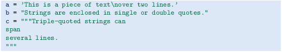
Observe here that we use a triple-quoted string, recognized by starting and ending with three single or double quotes: ’’’ or ″​″​″​. Triple-quoted strings are used for text that spans several lines.

In the print statement above, we print t in the f format, which by default implies six decimals; v0 is written in the .3E format, which implies three decimals and the number spans as narrow field as possible; and y is written with two decimals in decimal notation in as narrow field as possible. The output becomes

You should look at each number in the output and check the formatting in detail.

Format string syntax

Python offers all the functionality of the printf format and much more through a different syntax, often known as format string syntax. Let us illustrate this syntax on the one-line output previously used to show the printf construction. The corresponding format string syntax reads

The ‘‘slots’’ where variables are inserted are now recognized by curly braces rather than a percentage sign. The name of the variable is listed with an optional colon and format specifier of the same kind as was used for the printf format. The various variables and their values must be listed at the end as shown. This time the ‘‘slots’’ have names so the sequence of variables is not important.

The multi-line example is written as follows in this alternative format:

The newline character

We often want a computer program to write out text that spans several lines. In the last example we obtained such output by triple-quoted strings. We could also use ordinary single-quoted strings and a special character for indicating where line breaks should occur. This special character reads \n, i.e., a backslash followed by the letter n. The two print statements

result in identical output:

1.2 Computer Science Glossary

It is now time to pick up some important words that programmers use when they talk about programming: algorithm, application, assignment, blanks (whitespace), bug, code, code segment, code snippet, debug, debugging, execute, executable, implement, implementation, input, library, operating system, output, statement, syntax, user, verify, and verification. These words are frequently used in English in lots of contexts, yet they have a precise meaning in computer science.

Program and code are interchangeable terms. A code/program segment is a collection of consecutive statements from a program. Another term with similar meaning is code snippet. Many also use the word application in the same meaning as program and code. A related term is source code, which is the same as the text that constitutes the program. You find the source code of a program in one or more text files. (Note that text files normally have the extension .txt, while program files have an extension related to the programming language, e.g., .py for Python programs. The content of a .py file is, nevertheless, plain text as in a .txt file.)

We talk about running a program, or equivalently executing a program or executing a file. The file we execute is the file in which the program text is stored. This file is often called an executable or an application. The program text may appear in many files, but the executable is just the single file that starts the whole program when we run that file. Running a file can be done in several ways, for instance, by double-clicking the file icon, by writing the filename in a terminal window, or by giving the filename to some program. This latter technique is what we have used so far in this book: we feed the filename to the program python. That is, we execute a Python program by executing another program python, which interprets the text in our Python program file.

The term library is widely used for a collection of generally useful program pieces that can be applied in many different contexts. Having access to good libraries means that you do not need to program code snippets that others have already programmed (most probable in a better way!). There are huge numbers of Python libraries. In Python terminology, the libraries are composed of modules and packages. Section 1.4 gives a first glimpse of the math module, which contains a set of standard mathematical functions for $\sin x$, $\cos x$, $\ln x$, e^x, $\sinh x$, $\sin^{-1}x$, etc. Later, you will meet many other useful modules. Packages are just collections of modules. The standard Python distribution comes with a large number of modules and packages, but you can download many more from the Internet, see in particular www.python.org/pypi. Very often, when you encounter a programming task that is likely to occur in many other contexts, you can find a Python module where the job is already done. To mention just one example, say you need to compute how many days there are between two dates. This is a non-trivial task that lots of other programmers must have faced, so it is not a big surprise that Python comes with a module datetime to do calculations with dates.

The recipe for what the computer is supposed to do in a program is called algorithm. In the examples in the first couple of chapters in this book, the algorithms are so simple that we can hardly distinguish them from the program text itself, but later in the book we will carefully set up an algorithm before attempting to implement it in a program. This is useful when the algorithm is much more compact than the resulting program code. The algorithm in the current example consists of three steps:

• initialize the variables v₀, g, and t with numerical values,

• evaluate y according to the formula (1.1),

• print the y value to the screen.

The Python program is very close to this text, but some less experienced programmers may want to write the tasks in English before translating them to Python.

The implementation of an algorithm is the process of writing and testing a program. The testing phase is also known as verification: After the program text is written we need to verify that the program works correctly. This is a very important step that will receive substantial attention in the present book. Mathematical software produce numbers, and it is normally quite a challenging task to verify that the numbers are correct.

An error in a program is known as a bug, and the process of locating and removing bugs is called debugging. Many look at debugging as the most difficult and challenging part of computer programming. We have in fact devoted Appendix F to the art of debugging in this book. The origin of the strange terms bug and debugging can be found in Wikipedia³.

Programs are built of statements. There are many types of statements:

is an assignment statement, while

is a print statement. It is common to have one statement on each line, but it is possible to write multiple statements on one line if the statements are separated by semi-colon. Here is an example:

Although most newcomers to computer programming will think they understand the meaning of the lines in the above program, it is important to be aware of some major differences between notation in a computer program and notation in mathematics. When you see the equality sign = in mathematics, it has a certain interpretation as an equation ($x+2=5$) or a definition ($f(x)=x^{2}+1$). In a computer program, however, the equality sign has a quite different meaning, and it is called an assignment. The right-hand side of an assignment contains an expression, which is a combination of values, variables, and operators. When the expression is evaluated, it results in a value that the variable on the left-hand side will refer to. We often say that the right-hand side value is assigned to the variable on the left-hand side. In the current context it means that we in the first line assign the number 3 to the variable v0, 9.81 to g, and 0.6 to t. In the next line, the right-hand side expression v0*t - 0.5*g*t**2 is first evaluated, and the result is then assigned to the y variable.

Consider the assignment statement

This statement is mathematically false, but in a program it just means that we evaluate the right-hand side expression and assign its value to the variable y. That is, we first take the current value of y and add 3. The value of this operation is assigned to y. The old value of y is then lost.

You may think of the = as an arrow, y <- y+3, rather than an equality sign, to illustrate that the value to the right of the arrow is stored in the variable to the left of the arrow. In fact, the R programming language for statistical computing actually applies an arrow, many old languages (like Algol, Simula, and Pascal) used := to explicitly state that we are not dealing with a mathematical equality.

An example will illustrate the principle of assignment to a variable:

Running this program results in three numbers: 3, 7, 49. Go through the program and convince yourself that you understand what the result of each statement becomes.

A computer program must have correct syntax, meaning that the text in the program must follow the strict rules of the computer language for constructing statements. For example, the syntax of the print statement is the word print, followed by one or more spaces, followed by an expression of what we want to print (a Python variable, text enclosed in quotes, a number, for instance). Computers are very picky about syntax! For instance, a human having read all the previous pages may easily understand what this program does,

but the computer will find two errors in the last line: prinnt is an unknown instruction and Myvar is an undefined variable. Only the first error is reported (a syntax error), because Python stops the program once an error is found. All errors that Python finds are easy to remove. The difficulty with programming is to remove the rest of the errors, such as errors in formulas or the sequence of operations.

Blanks may or may not be important in Python programs. In Sect. 2.1.2 you will see that blanks are in some occasions essential for a correct program. Around = or arithmetic operators, however, blanks do not matter. We could hence write our program from Sect. 1.1.7 as

This is not a good idea because blanks are essential for easy reading of a program code, and easy reading is essential for finding errors, and finding errors is the difficult part of programming. The recommended layout in Python programs specifies one blank around =, +, and -, and no blanks around *, /, and **. Note that the blank after print is essential: print is a command in Python and printy is not recognized as any valid command. (Python will complain that printy is an undefined variable.) Computer scientists often use the term whitespace when referring to a blank. (To be more precise, blank is the character produced by the space bar on the keyboard, while whitespace denotes any character(s) that, if printed, do not print ink on the paper: a blank, a tabulator character (produced by backslash followed by t), or a newline character (produced by backslash followed by n). (The newline character is explained in Sect. 1.1.11.)

When we interact with computer programs, we usually provide some information to the program and get some information out. It is common to use the term input data, or just input, for the information that must be known on beforehand. The result from a program is similarly referred to as output data, or just output. In our example, v₀, g, and t constitute input, while y is output. All input data must be assigned values in the program before the output can be computed. Input data can be explicitly initialized in the program, as we do in the present example, or the data can be provided by the user through keyboard typing while the program is running (see Chap. 4). Output data can be printed in the terminal window, as in the current example, displayed as graphics on the screen, as done in Sect. 5.3, or stored in a file for later access, as explained in Sect. 4.6.

The word user usually has a special meaning in computer science: It means a human interacting with a program. You are a user of a text editor for writing Python programs, and you are a user of your own programs. When you write programs, it is difficult to imagine how other users will interact with the program. Maybe they provide wrong input or misinterpret the output. Making user-friendly programs is very challenging and depends heavily on the target audience of users. The author had the average reader of the book in mind as a typical user when developing programs for this book.

A central part of a computer is the operating system. This is actually a collection of programs that manages the hardware and software resources on the computer. There are three dominating operating systems today on computers: Windows, Mac OS X, and Linux. In addition, we have Android and iOS for handheld devices. Several versions of Windows have appeared since the 1990s: Windows 95, 98, 2000, ME, XP, Vista, Windows 7, and Windows 8. Unix was invented already in 1970 and comes in many different versions. Nowadays, two open source implementations of Unix, Linux and Free BSD Unix, are most common. The latter forms the core of the Mac OS X operating system on Macintosh machines, while Linux exists in slightly different flavors: Red Hat, Debian, Ubuntu, and OpenSuse to mention the most important distributions. We will use the term Unix in this book as a synonym for all the operating systems that inherit from classical Unix, such as Solaris, Free BSD, Mac OS X, and any Linux variant. As a computer user and reader of this book, you should know exactly what operating system you have.

The user’s interaction with the operation system is through a set of programs. The most widely used of these enable viewing the contents of folders or starting other programs. To interact with the operating system, as a user, you can either issue commands in a terminal window or use graphical programs. For example, for viewing the file contents of a folder you can run the command ls in a Unix terminal window or dir in a DOS (Windows) terminal window. The graphical alternatives are many, some of the most common are Windows Explorer on Windows, Nautilus and Konqueror on Unix, and Finder on Mac. To start a program, it is common to double-click on a file icon or write the program’s name in a terminal window.

1.3 Another Formula: Celsius-Fahrenheit Conversion

Our next example involves the formula for converting temperature measured in Celsius degrees to the corresponding value in Fahrenheit degrees:

$$F=\frac{9}{5}C+32$$

(1.3)

In this formula, C is the amount of degrees in Celsius, and F is the corresponding temperature measured in Fahrenheit. Our goal now is to write a computer program that can compute F from (1.3) when C is known.

1.3.1 Potential Error: Integer Division

Straightforward coding of the formula

A straightforward attempt at coding the formula (1.3) goes as follows:

The parentheses around 9/5 are not strictly needed, i.e., (9/5)*C is computationally identical to 9/5*C, but parentheses remove any doubt that 9/5*C could mean 9/(5*C). Section 1.3.4 has more information on this topic.

When run under Python version 2.x, the program prints the value 53. You can find the program in the file c2f_v1.py in the src/formulas folder in the folder tree of example programs from this book (downloaded from http://hplgit.github.com/scipro-primer). The v1 part of the name stands for version 1. Throughout this book, we will often develop several trial versions of a program, but remove the version number in the final version of the program.

Verifying the results

Testing the correctness is easy in this case since we can evaluate the formula on a calculator: $\frac{9}{5}\cdot 21+32$ is 69.8, not 53. What is wrong? The formula in the program looks correct!

Float and integer division

The error in our program above is one of the most common errors in mathematical software and is not at all obvious for a newcomer to programming. In many computer languages, there are two types of divisions: float division and integer division. Float division is what you know from mathematics: 9/5 becomes 1.8 in decimal notation.

Integer division $a/b$ with integers (whole numbers) a and b results in an integer that is truncated (or mathematically, rounded down). More precisely, the result is the largest integer c such that $bc\leq a$. This implies that 9/5 becomes 1 since $1\cdot 5=5\leq 9$ while $2\cdot 5=10> 9$. Another example is 1/5, which becomes 0 since $0\cdot 5\leq 1$ (and $1\cdot 5> 1$). Yet another example is 16/6, which results in 2 (try $2\cdot 6$ and $3\cdot 6$ to convince yourself). Many computer languages, including Fortran, C, C++, Java, and Python version 2, interpret a division operation a/b as integer division if both operands a and b are integers. If either a or b is a real (floating-point) number, a/b implies the standard mathematical float division. Other languages, such as MATLAB and Python version 3, interprets a/b as float division even if both operands are integers, or complex division if one of the operands is a complex number.

The problem with our program is the coding of the formula (9/5)*C + 32. This formula is evaluated as follows. First, 9/5 is calculated. Since 9 and 5 are interpreted by Python as integers (whole numbers), 9/5 is a division between two integers, and Python version 2 chooses by default integer division, which results in 1. Then 1 is multiplied by C, which equals 21, resulting in 21. Finally, 21 and 32 are added with 53 as result.

We shall very soon present a correct version of the temperature conversion program, but first it may be advantageous to introduce a frequently used term in Python programming: object.

1.3.2 Objects in Python

When we write

Python interprets the number 21 on the right-hand side of the assignment as an integer and creates an int (for integer) object holding the value 21. The variable C acts as a name for this int object. Similarly, if we write C = 21.0, Python recognizes 21.0 as a real number and therefore creates a float (for floating-point) object holding the value 21.0 and lets C be a name for this object. In fact, any assignment statement has the form of a variable name on the left-hand side and an object on the right-hand side. One may say that Python programming is about solving a problem by defining and changing objects.

At this stage, you do not need to know what an object really is, just think of an int object as a collection, say a storage box, with some information about an integer number. This information is stored somewhere in the computer’s memory, and with the name C the program gets access to this information. The fundamental issue right now is that 21 and 21.0 are identical numbers in mathematics, while in a Python program 21 gives rise to an int object and 21.0 to a float object.

There are lots of different object types in Python, and you will later learn how to create your own customized objects. Some objects contain a lot of data, not just an integer or a real number. For example, when we write

a str (string) object, without a name, is first made of the text between the quotes and then this str object is printed. We can alternatively do this in two steps:

1.3.3 Avoiding Integer Division

As a quite general rule of thumb, one should be careful to avoid integer division when programming mathematical formulas. In the rare cases when a mathematical algorithm does make use of integer division, one should use a double forward slash, //, as division operator, because this is Python’s way of explicitly indicating integer division.

Python version 3 has no problem with unintended integer division, so the problem only arises with Python version 2 (and many other common languages for scientific computing). There are several ways to avoid integer division with the plain / operator. The simplest remedy in Python version 2 is to write

This import statement must be present in the beginning of every file where the / operator always shall imply float division. Alternatively, one can run a Python program someprogram.py from the command line with the argument -Qnew to the Python interpreter:

A more widely applicable method, also in other programming languages than Python version 2, is to enforce one of the operands to be a float object. In the current example, there are several ways to do this:

In the first two lines, one of the operands is written as a decimal number, implying a float object and hence float division. In the last line, float(C)*9 means float times int, which results in a float object, and float division is guaranteed.

A related construction,

does not work correctly, because 9/5 is evaluated by integer division, yielding 1, before being multiplied by a float representation of C (see next section for how compound arithmetic operations are calculated). In other words, the formula reads F=C+32, which is wrong.

We now understand why the first version of the program does not work and what the remedy is. A correct program is

Instead of 9.0 we may just write 9. (the dot implies a float interpretation of the number). The program is available in the file c2f.py. Try to run it – and observe that the output becomes 69.8, which is correct.

Locating potential integer division

Running a Python program with the -Qwarnall argument, say

will print out a warning every time an integer division expression is encountered in Python version 2.

Remark

We could easily have run into problems in our very first programs if we instead of writing the formula $\frac{1}{2}gt^{2}$ as 0.5*g*t**2 wrote (1/2)*g*t**2. This term would then always be zero!

1.3.4 Arithmetic Operators and Precedence

Formulas in Python programs are usually evaluated in the same way as we would evaluate them mathematically. Python proceeds from left to right, term by term in an expression (terms are separated by plus or minus). In each term, power operations such as a^b, coded as a**b, has precedence over multiplication and division. As in mathematics, we can use parentheses to dictate the way a formula is evaluated. Below are two illustrations of these principles.

• 5/9+2*a**4/2: First 5/9 is evaluated (as integer division, giving 0 as result), then a⁴ (a**4) is evaluated, then 2 is multiplied with a⁴, that result is divided by 2, and the answer is added to the result of the first term. The answer is therefore a**4.

• 5/(9+2)*a**(4/2): First $5\over 9+2$ is evaluated (as integer division, yielding 0), then 4/2 is computed (as integer division, yielding 2), then a**2 is calculated, and that number is multiplied by the result of 5/(9+2). The answer is thus always zero.

As evident from these two examples, it is easy to unintentionally get integer division in formulas. Although integer division can be turned off in Python, we think it is important to be strongly aware of the integer division concept and to develop good programming habits to avoid it. The reason is that this concept appears in so many common computer languages that it is better to learn as early as possible how to deal with the problem rather than using a Python-specific feature to remove the problem.

1.4 Evaluating Standard Mathematical Functions

Mathematical formulas frequently involve functions such as sin, cos, tan, sinh, cosh, exp, log, etc. On a pocket calculator you have special buttons for such functions. Similarly, in a program you also have ready-made functionality for evaluating these types of mathematical functions. One could in principle write one’s own program for evaluating, e.g., the $\sin(x)$ function, but how to do this in an efficient way is a non-trivial topic. Experts have worked on this problem for decades and implemented their best recipes in pieces of software that we should reuse. This section tells you how to reach sin, cos, and similar functions in a Python context.

1.4.1 Example: Using the Square Root Function

Problem

Consider the formula for the height y of a ball in vertical motion, with initial upward velocity v₀:

$$y_{c}=v_{0}t-\frac{1}{2}gt^{2},$$

where g is the acceleration of gravity and t is time. We now ask the question: How long time does it take for the ball to reach the height y_c? The answer is straightforward to derive. When $y=y_{c}$ we have

$$y_{c}=v_{0}t-\frac{1}{2}gt^{2}\thinspace.$$

We recognize that this equation is a quadratic equation, which we must solve with respect to t. Rearranging,

$$\frac{1}{2}gt^{2}-v_{0}t+y_{c}=0,$$

and using the well-known formula for the two solutions of a quadratic equation, we find

$$t_{1}=\left({v_{0}-\sqrt{v_{0}^{2}-2gy_{c}}}\right)/g,\quad t_{2}=\left({v_{0}+\sqrt{v_{0}^{2}-2gy_{c}}}\right)/g\thinspace.$$

(1.4)

There are two solutions because the ball reaches the height y_c on its way up $(t=t_{1}$) and on its way down ($t=t_{2}> t_{1}$).

The program

To evaluate the expressions for t₁ and t₂ from (1.4) in a computer program, we need access to the square root function. In Python, the square root function and lots of other mathematical functions, such as sin, cos, sinh, exp, and log, are available in a module called math. We must first import the module before we can use it, that is, we must write import math. Thereafter, to take the square root of a variable a, we can write math.sqrt(a). This is demonstrated in a program for computing t₁ and t₂:

The output from this program becomes

You can find the program as the file ball_yc.py in the src/formulas folder.

Two ways of importing a module

The standard way to import a module, say math, is to write

and then access individual functions in the module with the module name as prefix as in

People working with mathematical functions often find math.sqrt(y) less pleasing than just sqrt(y). Fortunately, there is an alternative import syntax that allows us to skip the module name prefix. This alternative syntax has the form from module import function. A specific example is

Now we can work with sqrt directly, without the math. prefix. More than one function can be imported:

Sometimes one just writes

to import all functions in the math module. This includes sin, cos, tan, asin, acos, atan, sinh, cosh, tanh, exp, log (base e), log10 (base 10), sqrt, as well as the famous numbers e and pi. Importing all functions from a module, using the asterisk (*) syntax, is convenient, but this may result in a lot of extra names in the program that are not used. It is in general recommended not to import more functions than those that are really used in the program. Nevertheless, the convenience of the compact from math import * syntax occasionally wins over the general recommendation among practitioners – and in this book.

With a from math import sqrt statement we can write the formulas for the roots in a more pleasing way:

Import with new names

Imported modules and functions can be given new names in the import statement, e.g.,

In Python, everything is an object, and variables refer to objects, so new variables may refer to modules and functions as well as numbers and strings. The examples above on new names can also be coded by introducing new variables explicitly:

1.4.2 Example: Computing with $\sinh x$

Our next examples involve calling some more mathematical functions from the math module. We look at the definition of the $\sinh(x)$ function:

$$\sinh(x)=\frac{1}{2}\left(e^{x}-e^{-x}\right)\thinspace.$$

(1.5)

We can evaluate $\sinh(x)$ in three ways: i) by calling math.sinh, ii) by computing the right-hand side of (1.5), using math.exp, or iii) by computing the right-hand side of (1.5) with the aid of the power expressions math.e**x and math.e**(-x). A program doing these three alternative calculations is found in the file 3sinh.py. The core of the program looks like this:

The output from the program shows that all three computations give identical results:

1.4.3 A First Glimpse of Rounding Errors

The previous example computes a function in three different yet mathematically equivalent ways, and the output from the print statement shows that the three resulting numbers are equal. Nevertheless, this is not the whole story. Let us try to print out r1, r2, r3 with 16 decimals:

This statement leads to the output

Now r1 and r2 are equal, but r3 is different! Why is this so?

Our program computes with real numbers, and real numbers need in general an infinite number of decimals to be represented exactly. The computer truncates the sequence of decimals because the storage is finite. In fact, it is quite standard to keep only 17 digits in a real number on a computer. Exactly how this truncation is done is not explained in this book, but you read more on Wikipedia⁴. For now the purpose is to notify the reader that real numbers on a computer often have a small error. Only a few real numbers can be represented exactly, the rest of the real numbers are only approximations.

For this reason, most arithmetic operations involve inaccurate real numbers, resulting in inaccurate calculations. Think of the following two calculations: $1/49\cdot 49$ and $1/51\cdot 51$. Both expressions are identical to 1, but when we perform the calculations in Python,

the result becomes

The reason why we do not get exactly 1.0 as answer in the first case is because 1/49 is not correctly represented in the computer. Also 1/51 has an inexact representation, but the error does not propagate to the final answer.

To summarize, errors in floating-point numbers may propagate through mathematical calculations and result in answers that are only approximations to the exact underlying mathematical values. The errors in the answers are commonly known as rounding errors. As soon as you use Python interactively as explained in the next section, you will encounter rounding errors quite often.

Python has a special module decimal and the SymPy package has an alternative module mpmath, which allow real numbers to be represented with adjustable accuracy so that rounding errors can be made as small as desired (an example appears at the end of Sect. 3.1.12). However, we will hardly use such modules because approximations implied by many mathematical methods applied throughout this book normally lead to (much) larger errors than those caused by rounding.

1.5 Interactive Computing

A particular convenient feature of Python is the ability to execute statements and evaluate expressions interactively. The environments where you work interactively with programming are commonly known as Python shells. The simplest Python shell is invoked by just typing python at the command line in a terminal window. Some messages about Python are written out together with a prompt >>>, after which you can issue commands. Let us try to use the interactive shell as a calculator. Type in 3*4.5-0.5 and then press the Return key to see Python’s response to this expression:

The text on a line after >>> is what we write (shell input) and the text without the >>> prompt is the result that Python calculates (shell output). It is easy, as explained below, to recover previous input and edit the text. This editing feature makes it convenient to experiment with statements and expressions.

1.5.1 Using the Python Shell

The program from Sect. 1.1.7 can be typed in line by line in the interactive shell:

We can now easily calculate an y value corresponding to another (say) v0 value: hit the up arrow key to recover previous statements, repeat pressing this key until the v0 = 5 statement is displayed. You can then edit the line, e.g., to

Press return to execute this statement. You can control the new value of v0 by either typing just v0 or print v0:

The next step is to recompute y with this new v0 value. Hit the up arrow key multiple times to recover the statement where y is assigned, press the Return key, and write y or print y to see the result of the computation:

The reason why we get two slightly different results is that typing just y prints out all the decimals that are stored in the computer (16), while print y writes out y with fewer decimals. As mentioned in Sect. 1.4.3 computations on a computer often suffer from rounding errors. The present calculation is no exception. The correct answer is 1.8342, but rounding errors lead to a number that is incorrect in the 16th decimal. The error is here $4\cdot 10^{-16}$.

1.5.2 Type Conversion

Often you can work with variables in Python without bothering about the type of objects these variables refer to. Nevertheless, we encountered a serious problem in Sect. 1.3.1 with integer division, which forced us to be careful about the types of objects in a calculation. The interactive shell is very useful for exploring types. The following example illustrates the type function and how we can convert an object from one type to another.

First, we create an int object bound to the name C and check its type by calling type(C):

We convert this int object to a corresponding float object:

In the statement C = float(C) we create a new object from the original object referred to by the name C and bind it to the same name C. That is, C refers to a different object after the statement than before. The original int with value 21 cannot be reached anymore (since we have no name for it) and will be automatically deleted by Python.

We may also do the reverse operation, i.e., convert a particular float object to a corresponding int object:

In general, one can convert a variable v to type MyType by writing v=MyType(v), if it makes sense to do the conversion.

In the last input we tried to convert a float to an int, and this operation implied stripping off the decimals. Correct conversion according to mathematical rounding rules can be achieved with help of the round function:

1.5.3 IPython

There exist several improvements of the standard Python shell presented in Sect. 1.5. The author advocates IPython as the preferred interactive shell. You will then need to have IPython installed. Typing ipython in a terminal window starts the shell. The (default) prompt in IPython is not >>> but In [X]:, where X is the number of the present input command. The most widely used features of IPython are summarized below.

Running programs

Python programs can be run from within the shell:

This command requires that you have taken a cd to the folder where the ball2.py program is located and started IPython from there.

On Windows you may, as an alternative to starting IPython from a DOS or PowerShell window, double click on the IPython desktop icon or use the Start menu. In that case, you must move to the right folder where your program is located. This is done by the os.chdir (change directory) command. Typically, you write something like

if the ball2.py program is located in the folder div under My Documents of user me. Note the r before the quote in the string: it is required to let a backslash really mean the backslash character. If you end up typing the os.chdir command every time you enter an IPython shell, this command (and others) can be placed in a startup file such that they are automatically executed when you launch IPython.

Inside IPython you can invoke any operating system command. This allows us to navigate to the right folder above using Unix or Windows (cd) rather than Python (os.chdir):

We recommend running all your Python programs from the IPython shell. Especially when something goes wrong, IPython can help you to examine the state of variables so that you become quicker to locate bugs.

Typesetting convention for executing Python programs

In the rest of the book, we just write the program name and the output when we illustrate the execution of a program:

You then need to write run before the program name if you execute the program in IPython, or if you prefer to run the program directly in a terminal window, you need to write python prior to the program name. Appendix H.5 describes various other ways to run a Python program.

Quick recovery of previous output

The results of the previous statements in an interactive IPython session are available in variables of the form _iX (underscore, i, and a number X), where X is 1 for the last statement, 2 for the second last statement, and so forth. Short forms are _ for _i1, __ for _i2, and ___ for _i3. The output from the In [1] input above is 1.2342. We can now refer to this number by an underscore and, e.g., multiply it by 10:

Output from Python statements or expressions in IPython are preceded by Out[X] where X is the command number corresponding to the previous In [X] prompt. When programs are executed, as with the run command, or when operating system commands are run (as shown below), the output is from the operating system and then not preceded by any Out[X] label.

The command history from previous IPython sessions is available in a new session. This feature makes it easy to modify work from a previous session by just hitting the up-arrow to recall commands and edit them as necessary.

Tab completion

Pressing the TAB key will complete an incompletely typed variable name. For example, after defining my_long_variable_name = 4, write just my at the In [4]: prompt below, and then hit the TAB key. You will experience that my is immediately expanded to my_long_variable_name. This automatic expansion feature is called TAB completion and can save you from quite some typing.

Recovering previous commands

You can walk through the command history by typing Ctrl+p or the up arrow for going backward or Ctrl+n or the down arrow for going forward. Any command you hit can be edited and re-executed. Also commands from previous interactive sessions are stored in the command history.

Running Unix/Windows commands

Operating system commands can be run from IPython. Below we run the three Unix commands date, ls (list files), mkdir (make directory), and cd (change directory):

If you have defined Python variables with the same name as operating system commands, e.g., date=30, you must write !date to run the corresponding operating system command.

IPython can do much more than what is shown here, but the advanced features and the documentation of them probably do not make sense before you are more experienced with Python – and with reading manuals.

Typesetting of interactive shells in this book

In the rest of the book we will apply the >>> prompt in interactive sessions instead of the input and output prompts as used by default by IPython, simply because most Python books and electronic manuals use >>> to mark input in interactive shells. However, when you sit by the computer and want to use an interactive shell, we recommend using IPython, and then you will see the In [X] prompt instead of >>>.

Notebooks

A particularly interesting feature of IPython is the notebook, which allows you to record and replay exploratory interactive sessions with a mix of text, mathematics, Python code, and graphics. See Sect. H.4 for a quick introduction to IPython notebooks.

1.6 Complex Numbers

Suppose $x^{2}=2$. Then most of us are able to find out that $x=\sqrt{2}$ is a solution to the equation. The more mathematically interested reader will also remark that $x=-\sqrt{2}$ is another solution. But faced with the equation $x^{2}=-2$, very few are able to find a proper solution without any previous knowledge of complex numbers. Such numbers have many applications in science, and it is therefore important to be able to use such numbers in our programs.

On the following pages we extend the previous material on computing with real numbers to complex numbers. The text is optional, and readers without knowledge of complex numbers can safely drop this section and jump to Sect. 1.8.

A complex number is a pair of real numbers a and b, most often written as $a+bi$, or $a+ib$, where i is called the imaginary unit and acts as a label for the second term. Mathematically, $i=\sqrt{-1}$. An important feature of complex numbers is definitely the ability to compute square roots of negative numbers. For example, $\sqrt{-2}=\sqrt{2}i$ (i.e., $\sqrt{2}\sqrt{-1}$). The solutions of $x^{2}=-2$ are thus $x_{1}=+\sqrt{2}i$ and $x_{2}=-\sqrt{2}i$.

There are rules for addition, subtraction, multiplication, and division between two complex numbers. There are also rules for raising a complex number to a real power, as well as rules for computing $\sin z$, $\cos z$, $\tan z$, e^z, $\ln z$, $\sinh z$, $\cosh z$, $\tanh z$, etc. for a complex number $z=a+ib$. We assume in the following that you are familiar with the mathematics of complex numbers, at least to the degree encountered in the program examples.

$$\hbox{let }u=a+bi\hbox{ and }v=c+di$$

The following rules reflect complex arithmetics:

$$\begin{aligned}\displaystyle u&\displaystyle=v\quad\Rightarrow\quad a=c,\ b=d\\ \displaystyle-u&\displaystyle=-a-bi\\ \displaystyle u^{*}&\displaystyle\equiv a-bi\quad\hbox{(complex conjugate)}\\ \displaystyle u+v&\displaystyle=(a+c)+(b+d)i\\ \displaystyle u-v&\displaystyle=(a-c)+(b-d)i\\ \displaystyle uv&\displaystyle=(ac-bd)+(bc+ad)i\\ \displaystyle u/v&\displaystyle=\frac{ac+bd}{c^{2}+d^{2}}+\frac{bc-ad}{c^{2}+d^{2}}i\\ \displaystyle|u|&\displaystyle=\sqrt{a^{2}+b^{2}}\\ \displaystyle e^{iq}&\displaystyle=\cos q+i\sin q\end{aligned}$$

1.6.1 Complex Arithmetics in Python

Python supports computation with complex numbers. The imaginary unit is written as j in Python, instead of i as in mathematics. A complex number $2-3i$ is therefore expressed as (2-3j) in Python. We remark that the number i is written as 1j, not just j. Below is a sample session involving definition of complex numbers and some simple arithmetics:

A complex object s has functionality for extracting the real and imaginary parts as well as computing the complex conjugate:

1.6.2 Complex Functions in Python

Taking the sine of a complex number does not work:

The reason is that the sin function from the math module only works with real (float) arguments, not complex. A similar module, cmath, defines functions that take a complex number as argument and return a complex number as result. As an example of using the cmath module, we can demonstrate that the relation $\sin(ai)=i\sinh a$ holds:

Another relation, $e^{iq}=\cos q+i\sin q$, is exemplified next:

1.6.3 Unified Treatment of Complex and Real Functions

The cmath functions always return complex numbers. It would be nice to have functions that return a float object if the result is a real number and a complex object if the result is a complex number. The Numerical Python package has such versions of the basic mathematical functions known from math and cmath. By taking a

one obtains access to these flexible versions of mathematical functions. The functions also get imported by any of the statements

A session will illustrate what we obtain. Let us first use the sqrt function in the math module:

If we now import sqrt from cmath,

the previous sqrt function is overwritten by the new one. More precisely, the name sqrt was previously bound to a function sqrt from the math module, but is now bound to another function sqrt from the cmath module. In this case, any square root results in a complex object:

If we now take

we import (among other things) a new sqrt function. This function is slower than the versions from math and cmath, but it has more flexibility since the returned object is float if that is mathematically possible, otherwise a complex is returned:

As a further illustration of the need for flexible treatment of both complex and real numbers, we may code the formulas for the roots of a quadratic function $f(x)=ax^{2}+bx+c$:

Using the up arrow, we may go back to the definitions of the coefficients and change them so the roots become real numbers:

Going back to the computations of r1 and r2 and performing them again, we get

That is, the two results are float objects. Had we applied sqrt from cmath, r1 and r2 would always be complex objects, while sqrt from the math module would not handle the first (complex) case.

1.7 Symbolic Computing

Python has a package SymPy for doing symbolic computing, such as symbolic (exact) integration, differentiation, equation solving, and expansion of Taylor series, to mention some common operations in mathematics. We shall here only give a glimpse of SymPy in action with the purpose of drawing attention to this powerful part of Python.

For interactive work with SymPy it is recommended to either use IPython or the special, interactive shell isympy, which is installed along with SymPy itself.

Below we shall explicitly import each symbol we need from SymPy to emphasize that the symbol comes from that package. For example, it will be important to know whether sin means the sine function from the math module, aimed at real numbers, or the special sine function from sympy, aimed at symbolic expressions.

1.7.1 Basic Differentiation and Integration

The following session shows how easy it is to differentiate a formula $v_{0}t-\frac{1}{2}gt^{2}$ with respect to t and integrate the answer to get the formula back:

Note here that t is a symbolic variable (not a float as it is in numerical computing), and y (like y2) is a symbolic expression (not a float as it would be in numerical computing).

A very convenient feature of SymPy is that symbolic expressions can be turned into ordinary Python functions via lambdify. (Python functions are introduced in Chap. 3, but when discussing SymPy here in the present chapter, it is very natural to explain how lambdify can transform symbolic expressions back to ordinary numerical Python expressions.) Let us take the dydt expression above and turn it into a Python function v(t, v0, g) for numerical computing:

1.7.2 Equation Solving

A linear equation defined through an expression e that is zero, can be solved by solve(e, t), if t is the unknown (symbol) in the equation. Here we may find the roots of y = 0:

We can easily check the answer by inserting the roots in y. Inserting an expression e2 for e1 in some expression e is done by e.subs(e1, e2). In our case we check that

1.7.3 Taylor Series and More

A Taylor polynomial of order n for an expression e in a variable t around the point t0 is computed by e.series(t, t0, n). Testing this on e^t and $e^{\sin(t)}$ gives

Output of mathematical expressions in the LaTeX typesetting system is possible:

Finally, we mention that there are tools for expanding and simplifying expressions:

Later chapters utilize SymPy where it can save some algebraic work, but this book is almost exclusively devoted to numerical computing.

1.8 Summary

1.8.1 Chapter Topics

Programs must be accurate!

A program is a collection of statements stored in a text file. Statements can also be executed interactively in a Python shell. Any error in any statement may lead to termination of the execution or wrong results. The computer does exactly what the programmer tells the computer to do!

Variables

The statement

defines a variable with the name some_variable which refers to an object obj. Here obj may also represent an expression, say a formula, whose value is a Python object. For example, 1+2.5 involves the addition of an int object and a float object, resulting in a float object. Names of variables can contain upper and lower case English letters, underscores, and the digits from 0 to 9, but the name cannot start with a digit. Nor can a variable name be a reserved word in Python.

If there exists a precise mathematical description of the problem to be solved in a program, one should choose variable names that are in accordance with the mathematical description. Quantities that do not have a defined mathematical symbol, should be referred to by descriptive variables names, i.e., names that explain the variable’s role in the program. Well-chosen variable names are essential for making a program easy to read, easy to debug, and easy to extend. Well-chosen variable names also reduce the need for comments.

Comment lines

Everything after # on a line is ignored by Python and used to insert free running text, known as comments. The purpose of comments is to explain, in a human language, the ideas of (several) forthcoming statements so that the program becomes easier to understand for humans. Some variables whose names are not completely self-explanatory also need a comment.

Object types

There are many different types of objects in Python. In this chapter we have worked with the following types.

• Integers (whole numbers, object type int):

  

• Floats (decimal numbers, object type float):

  

• Strings (pieces of text, object type str):

  

• Complex numbers (object type complex):

  

Operators

Operators in arithmetic expressions follow the rules from mathematics: power is evaluated before multiplication and division, while the latter two are evaluated before addition and subtraction. These rules are overridden by parentheses. We suggest using parentheses to group and clarify mathematical expressions, also when not strictly needed.

Particular attention must be paid to coding fractions, since the division operator / often needs extra parentheses that are not necessary in the mathematical notation for fractions (compare $\frac{a}{b+c}$ with a/(b+c) and a/b+c).

Common mathematical functions

The math module contains common mathematical functions for real numbers. Modules must be imported before they can be used. The three types of alternative module import go as follows:

Print

To print the result of calculations in a Python program to a terminal window, we apply the print command, i.e., the word print followed by a string enclosed in quotes, or just a variable:

Several objects can be printed in one statement if the objects are separated by commas. A space will then appear between the output of each object:

The printf syntax enables full control of the formatting of real numbers and integers:

Here, a, b, and c are of type float and formatted as compactly as possible (%g for a), in scientific notation with 4 decimals in a field of width 12 (%12.4E for b), and in decimal notation with two decimals in as compact field as possible (%.2f for c). The variable d is an integer (int) written in a field of width 5 characters (%5d).

Be careful with integer division!

A common error in mathematical computations is to divide two integers, because this results in integer division (in Python 2).

• Any number written without decimals is treated as an integer. To avoid integer division, ensure that every division involves at least one real number, e.g., 9/5 is written as 9.0/5, 9./5, 9/5., or 9/5.0.

• In expressions with variables, a/b, ensure that a or b is a float object, and if not (or uncertain), do an explicit conversion as in float(a)/b to guarantee float division.

• If integer division is desired, use a double slash: a//b.

• Python 3 treats a/b as float division also when a and b are integers.

Complex numbers

Values of complex numbers are written as (X+Yj), where X is the value of the real part and Y is the value of the imaginary part. One example is (4-0.2j). If the real and imaginary parts are available as variables r and i, a complex number can be created by complex(r, i).

The cmath module must be used instead of math if the argument is a complex variable. The numpy package offers similar mathematical functions, but with a unified treatment of real and complex variables.

Terminology

Some Python and computer science terms briefly covered in this chapter are

• object: anything that a variable (name) can refer to, such as a number, string, function, or module (but objects can exist without being bound to a name: print ’Hello!’ first makes a string object of the text in quotes and then the contents of this string object, without a name, is printed)

• variable: name of an object

• statement: an instruction to the computer, usually written on a line in a Python program (multiple statements on a line must be separated by semicolons)

• expression: a combination of numbers, text, variables, and operators that results in a new object, when being evaluated

• assignment: a statement binding an evaluated expression (object) to a variable (name)

• algorithm: detailed recipe for how to solve a problem by programming

• code: program text (or synonym for program)

• implementation: same as code

• executable: the file we run to start the program

• verification: providing evidence that the program works correctly

• debugging: locating and correcting errors in a program

1.8.2 Example: Trajectory of a Ball

Problem

What is the trajectory of a ball that is thrown or kicked with an initial velocity v₀ making an angle θ with the horizontal? This problem can be solved by basic high school physics as you are encouraged to do in Exercise 1.13. The ball will follow a trajectory $y=f(x)$ through the air where

$$f(x)=x\tan\theta-{1\over 2v_{0}^{2}}{gx^{2}\over\cos^{2}\theta}+y_{0}\thinspace.$$

(1.6)

In this expression, x is a horizontal coordinate, g is the acceleration of gravity, v₀ is the size of the initial velocity that makes an angle θ with the x axis, and $(0,y_{0})$ is the initial position of the ball. Our programming goal is to make a program for evaluating (1.6). The program should write out the value of all the involved variables and what their units are.

We remark that the formula (1.6) neglects air resistance. Exercise 1.11 explores how important air resistance is. For a soft kick ($v_{0}=30$ km/h) of a football, the gravity force is much larger than the air resistance, but for a hard kick, air resistance may be as important as gravity.

Solution

We use the SI system and assume that v₀ is given in km/h; $g=9.81\hbox{m/s}^{2}$; x, y, and y₀ are measured in meters; and θ in degrees. The program has naturally four parts: initialization of input data, import of functions and π from math, conversion of v₀ and θ to m/s and radians, respectively, and evaluation of the right-hand side expression in (1.6). We choose to write out all numerical values with one decimal. The complete program is found in the file trajectory.py:

The backslash in the triple-quoted multi-line string makes the string continue on the next line without a newline. This means that removing the backslash results in a blank line above the v0 line and a blank line between the x and y lines in the output on the screen. Another point to mention is the expression 1/(2*v0**2), which might seem as a candidate for unintended integer division. However, the conversion of v0 to m/s involves a division by 3.6, which results in v0 being float, and therefore 2*v0**2 being float. The rest of the program should be self-explanatory at this stage in the book.

We can execute the program in IPython or an ordinary terminal window and watch the output:

1.8.3 About Typesetting Conventions in This Book

This version of the book applies different design elements for different types of ‘‘computer text’’. Complete programs and parts of programs (snippets) are typeset with a light blue background. A snippet looks like this:

A complete program has an additional, slightly darker frame:

As a reader of this book, you may wonder if a code shown is a complete program you can try out or if it is just a part of a program (a snippet) so that you need to add surrounding statements (e.g., import statements) to try the code out yourself. The appearance of a vertical line to the left or not will then quickly tell you what type of code you see.

An interactive Python session is typeset as

Running a program, say ball_yc.py, in the terminal window, followed by some possible output is typeset as

Recall from Sect. 1.5.3 that we just write the program name. A real execution demands prefixing the program name by python in a terminal window, or by run if you run the program from an interactive IPython session. We refer to Appendix H.5 for more complete information on running Python programs in different ways.

Sometimes just the output from a program is shown, and this output appears as plain computer text:

Files containing data are shown in a similar way in this book:

Style guide for Python code

This book presents Python code that is (mostly) in accordance with the official Style Guide for Python Code⁵, known in the Python community as PEP8. Some exceptions to the rules are made to make code snippets shorter: multiple imports on one line and less blank lines.

1.9 Exercises

About solving exercises

There is only one way to learn programming: you have to program yourself. This means that you have to do a lot of exercises! Reading this book is necessary to learn about the Python syntax and studying the examples in depth is necessary to grasp how to think about programming and solving problems. But the main effort in the learning process is your work with exercises or your own programming projects.

Solving an exercise is a three-stage procedure. First, you have to study the text in the exercise carefully to understand what the problem is about. Programming exercises, especially in this book, are about a problem setting that has to be thoroughly understood before it makes sense to understand the specific questions in the exercise. The second phase is to write the program. The more efforts you put into the first phase, the easier it will be to find the right statements and write the code. The third and final stage is to test the program and remove errors (known as debugging and verification from Sect. 1.2). This is by far the greatest challenge for beginners. Very often, especially for newcomers to programming, it boils down to writing out the result of every statement and checking these results carefully by playing computer with pen and paper.

Beginners often underestimate the amount of work required in the first and third stage and instead try to do the second stage (i.e., write the program) as quickly as possible. The more work you put into the first stage, the easier it will be to find an example in this book or elsewhere that is similar to the exercise and that can help you get started. And the more work you put into stage three up front, with constructing a test case, the better your understanding of the statements will be and the fewer errors you will commit. Experience will prove that all these assertions are right!

Most exercises are associated with a filename, e.g., myexer. If the answer to the exercise is a Python program, you should store the program in a file myexer.py. If the answer can be an explanation, you may store it in a plain text file, myexer.txt, or write the text in a word processor and produce a PDF file (myexer_OnlinePDF.pdf).

When you hand in exercises to teaching assistants, it is often a requirement that a trial run of the program is inserted at the end of the code. This means that you run some case with known result, direct the output to a file result,

and copy the contents of result to a triple-quoted string with appropriate comments after the statements of the program. Here is an example of a program with its trial run inserted:

The trial run demonstrates that the program runs and produces correct results in a test case.

Exercise 1.1 (Compute 1+1)

The first exercise concerns some very basic mathematics and programming: assign the result of 1$+$1 to a variable and print the value of that variable.

Filename: 1plus1.

Exercise 1.2 (Write a Hello World program)

Almost all books about programming languages start with a very simple program that prints the text Hello, World! to the screen. Make such a program in Python.

Filename: hello_world.

Exercise 1.3 (Derive and compute a formula)

Can a newborn baby in Norway expect to live for one billion (10⁹) seconds? Write a Python program for doing arithmetics to answer the question.

Filename: seconds2years.

Exercise 1.4 (Convert from meters to British length units)

Make a program where you set a length given in meters and then compute and write out the corresponding length measured in inches, in feet, in yards, and in miles. Use that one inch is 2.54 cm, one foot is 12 inches, one yard is 3 feet, and one British mile is 1760 yards. For verification, a length of 640 meters corresponds to 25196.85 inches, 2099.74 feet, 699.91 yards, or 0.3977 miles.

Filename: length_conversion.

Exercise 1.5 (Compute the mass of various substances)

The density of a substance is defined as $\varrho=m/V$, where m is the mass of a volume V. Compute and print out the mass of one liter of each of the following substances whose densities in $\hbox{g/cm}^{3}$ are found in the file src/files/densities.datFootnote

http://tinyurl.com/pwyasaa/files/densities.dat

: iron, air, gasoline, ice, the human body, silver, and platinum.

Filename: 1liter.

Exercise 1.6 (Compute the growth of money in a bank)

Let p be a bank’s interest rate in percent per year. An initial amount A has then grown to

$$A\left(1+{p\over 100}\right)^{n}$$

after n years. Make a program for computing how much money 1000 euros have grown to after three years with 5 percent interest rate.

Filename: interest_rate.

Exercise 1.7 (Find error(s) in a program)

Suppose somebody has written a simple one-line program for computing $\sin(1)$:

Create this program and try to run it. What is the problem?

Filename: find_errors_sin1.

Exercise 1.8 (Type in program text)

Type the following program in your editor and execute it. If your program does not work, check that you have copied the code correctly.

Filename: formulas_shapes.

Exercise 1.9 (Type in programs and debug them)

Type these short programs in your editor and execute them. When they do not work, identify and correct the erroneous statements.

• a) Does $\sin^{2}(x)+\cos^{2}(x)=1$?

  

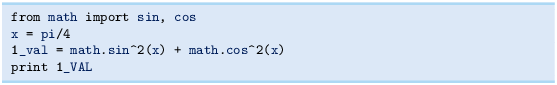
• b) Compute s in meters when $s=v_{0}t+\frac{1}{2}at^{2}$, with $v_{0}=3$ m/s, t = 1 s, $a=2\ \hbox{m/s}^{2}$.

  

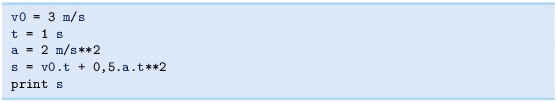
• c) Verify these equations:

  $$\begin{aligned}\displaystyle(a+b)^{2}&\displaystyle=a^{2}+2ab+b^{2}\\ \displaystyle(a-b)^{2}&\displaystyle=a^{2}-2ab+b^{2}\end{aligned}$$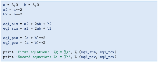

  

Filename: find_errors_programs.

Exercise 1.10 (Evaluate a Gaussian function)

The bell-shaped Gaussian function,

$$f(x)={1\over\sqrt{2\pi}\,s}\exp{\left[-\frac{1}{2}\left({x-m\over s}\right)^{2}\right]},$$

(1.7)

is one of the most widely used functions in science and technology. The parameters m and s > 0 are prescribed real numbers. Make a program for evaluating this function when m = 0, s = 2, and x = 1. Verify the program’s result by comparing with hand calculations on a calculator.

Filename: gaussian1.

Remarks

The function (1.7) is named after Carl Friedrich Gauss⁷, 1777–1855, who was a German mathematician and scientist, now considered as one of the greatest scientists of all time. He contributed to many fields, including number theory, statistics, mathematical analysis, differential geometry, geodesy, electrostatics, astronomy, and optics. Gauss introduced the function (1.7) when he analyzed probabilities related to astronomical data.

Exercise 1.11 (Compute the air resistance on a football)

The drag force, due to air resistance, on an object can be expressed as

$$F_{d}=\frac{1}{2}C_{D}\varrho AV^{2},$$

(1.8)

where $\varrho$ is the density of the air, V is the velocity of the object, A is the cross-sectional area (normal to the velocity direction), and C_D is the drag coefficient, which depends heavily on the shape of the object and the roughness of the surface.

The gravity force on an object with mass m is $F_{g}=mg$, where $g=9.81\,\hbox{m}\,\hbox{s}^{-2}$.

We can use the formulas for F_d and F_g to study the importance of air resistance versus gravity when kicking a football. The density of air is $\varrho=1.2\ \hbox{kg }\,{\hbox{m}}^{-3}$. We have $A=\pi a^{2}$ for any ball with radius a. For a football, a = 11 cm and the mass is 0.43 kg. The drag coefficient C_D varies with the velocity and can be taken as 0.4.

Make a program that computes the drag force and the gravity force on a football. Write out the forces with one decimal in units of Newton ($\hbox{N}=\hbox{kg}\,\hbox{m}/\hbox{s}^{2}$). Also print the ratio of the drag force and the gravity force. Define C_D, $\varrho$, A, V, m, g, F_d, and F_g as variables, and put a comment with the corresponding unit. Use the program to calculate the forces on the ball for a hard kick, $V=120\,\hbox{ km}/\hbox{h}$ and for a soft kick, $V=30\,\hbox{ km}/\hbox{h}$ (it is easy to mix inconsistent units, so make sure you compute with V expressed in m$/$s).

Filename: kick.

Exercise 1.12 (How to cook the perfect egg)

As an egg cooks, the proteins first denature and then coagulate. When the temperature exceeds a critical point, reactions begin and proceed faster as the temperature increases. In the egg white, the proteins start to coagulate for temperatures above 63 ${}^{\circ}$C, while in the yolk the proteins start to coagulate for temperatures above 70 ${}^{\circ}$C. For a soft boiled egg, the white needs to have been heated long enough to coagulate at a temperature above 63 ${}^{\circ}$C, but the yolk should not be heated above 70 ${}^{\circ}$C. For a hard boiled egg, the center of the yolk should be allowed to reach 70 ${}^{\circ}$C.

The following formula expresses the time t it takes (in seconds) for the center of the yolk to reach the temperature T_y (in Celsius degrees):

$$t=\frac{M^{2/3}c\rho^{1/3}}{K\pi^{2}(4\pi/3)^{2/3}}\ln\left[0.76\frac{T_{o}-T_{w}}{T_{y}-T_{w}}\right]\thinspace.$$

(1.9)

Here, M, ρ, c, and K are properties of the egg: M is the mass, ρ is the density, c is the specific heat capacity, and K is thermal conductivity. Relevant values are M = 47 g for a small egg and M = 67 g for a large egg, $\rho=1.038\,\hbox{g}\,\hbox{cm}^{-3}$, $c=3.7\,\hbox{ J}\,\hbox{g}^{-1}\,\hbox{K}^{-1}$, and $K=5.4\cdot 10^{-3}\,\hbox{W}\,\hbox{cm}^{-1}\,\hbox{K}^{-1}$. Furthermore, T_w is the temperature (in C degrees) of the boiling water, and T_o is the original temperature (in C degrees) of the egg before being put in the water. Implement the formula in a program, set $T_{w}=100$ ${}^{\circ}$C and $T_{y}=70$ ${}^{\circ}$C, and compute t for a large egg taken from the fridge ($T_{o}=4$ ${}^{\circ}$C) and from room temperature ($T_{o}=20$ ${}^{\circ}$C).

Filename: egg.

Exercise 1.13 (Derive the trajectory of a ball)

The purpose of this exercise is to explain how Equation (1.6) for the trajectory of a ball arises from basic physics. There is no programming in this exercise, just physics and mathematics.

The motion of the ball is governed by Newton’s second law:

$$F_{x} =ma_{x}$$

(1.10)

$$F_{y} =ma_{y}$$

(1.11)

where F_x and F_y are the sum of forces in the x and y directions, respectively, a_x and a_y are the accelerations of the ball in the x and y directions, and m is the mass of the ball. Let $(x(t),y(t))$ be the position of the ball, i.e., the horizontal and vertical coordinate of the ball at time t. There are well-known relations between acceleration, velocity, and position: the acceleration is the time derivative of the velocity, and the velocity is the time derivative of the position. Therefore we have that

$$a_{x} ={d^{2}x\over dt^{2}},$$

(1.12)

$$a_{y} ={d^{2}y\over dt^{2}}\thinspace.$$

(1.13)

If we assume that gravity is the only important force on the ball, $F_{x}=0$ and $F_{y}=-mg$.

Integrate the two components of Newton’s second law twice. Use the initial conditions on velocity and position,

$${d\over dt}x(0) =v_{0}\cos\theta,$$

(1.14)

$${d\over dt}y(0) =v_{0}\sin\theta,$$

(1.15)

$$x(0) =0,$$

(1.16)

$$y(0) =y_{0},$$

(1.17)

to determine the four integration constants. Write up the final expressions for $x(t)$ and $y(t)$. Show that if $\theta=\pi/2$, i.e., the motion is purely vertical, we get the formula (1.1) for the y position. Also show that if we eliminate t, we end up with the relation (1.6) between the x and y coordinates of the ball. You may read more about this type of motion in a physics book, e.g., [16].

Filename: trajectory.

Exercise 1.14 (Find errors in the coding of formulas)

Some versions of our program for calculating the formula (1.3) are listed below. Find the versions that will not work correctly and explain why in each case.

Filename: find_errors_division.

Exercise 1.15 (Explain why a program does not work)

Figure out why the following program does not work:

Filename: find_errors_vars.

Exercise 1.16 (Find errors in Python statements)

Try the following statements in an interactive Python shell. Explain why some statements fail and correct the errors.

Hint

It is wise to test the values of the expressions on the right-hand side, and the validity of the variable names, separately before you put the left- and right-hand sides together in statements. The last two statements work, but explaining why goes beyond what is treated in this chapter.

Filename: find_errors_syntax.

Exercise 1.17 (Find errors in the coding of a formula)

Given a quadratic equation,

$$ax^{2}+bx+c=0,$$

the two roots are

$$x_{1}={-b+\sqrt{b^{2}-4ac}\over 2a},\quad x_{2}={-b-\sqrt{b^{2}-4ac}\over 2a}\thinspace.$$

(1.18)

What are the problems with the following program?

Correct the program so that it solves the given equation.

Filename: find_errors_roots.

Exercise 1.18 (Find errors in a program)

What is the problem in the following program?

Filename: find_errors_tan.