Features as Keypoints and How Fuzzy Transforms Retrieve Them

Abstract

We are focused on a new fast and robust algorithm of image/signal feature extraction in the form of representative keypoints. We analyze various multi-scale representations of a one-dimensional signal in spaces with a closeness relation determined by a symmetric and positive semi-definite kernel. We show that kernels arising from generating functions of fuzzy partitions can be used in a scale space representation of a one-dimensional signal. We show that the reconstruction from the proposed multi-scale representations is of better quality than the reconstruction from MLP with almost double the number of neurons in 4 hidden layers. Finally, we propose a new algorithm of keypoints localization and description and test it on financial time series with high volatility.

1 Introduction

We are focused on a new fast and robust algorithm of image/signal feature extraction in the form of representative keypoints. This problem closely relates to the data processing by neural networks, extraction of stable features that are invariant under various geometric transformations.

Our motivation is supported by the recently published overview of the explainability of artificial intelligence [1], the authors of which pointed out that “The sophistication of AI-powered systems has lately increased to such an extent that almost no human intervention is required for their design and deployment. When decisions derived from such systems ultimately affect humans’ lives (as in e.g. medicine, law or defense), there is an emerging need for understanding how such decisions are furnished by AI methods.” They propose to link explainability to understanding how the data is processed by the model, which means how the results obtained contribute to solving the imposed problem. This forces us to focus on feature extraction because it is the first step in every machine learning algorithm.

Depending on feature extractors, we distinguish between local, semi-local, and non-local features. The character of their extraction (by means of convolution) depends on a receptive field of the corresponding kernel. The latter is connected with semantics of the extracted value and by this, contributes to the explainability. Therefore, to increase the level of explainability, we shall consciously select convolution kernels.

In image processing tasks, features are associated with keypoints and their descriptors. In early works, both were identified with local areas of the image that correspond to its content (not related to the background). Thus, the processing was computationally consuming and depending on many space-environment conditions: illumination, position, resolution, etc. In the seminal work [12], it was shown that invariant local features (Harris corners and their rotation invariant descriptors) can contribute to solving general problems of image recognition. In detail, an invariant image description in a neighborhood of a point can be described by the set of its convolutions with Gaussian derivatives. Because the Harris corner detector is sensitive to changes in image scale, it was expanded in [8] to the descriptor known in the literature as SIFT to achieve scale and rotation invariance and to provide reliable matching over a wide range of affine distortions. The publication of SIFT has inspired many modifications: SURF, PCA-SIFT, GLOH, Gauss-SIFT, etc., (see [7] and references therein), aimed at improving its efficiency in various senses: reliability, computation time, etc. However, the main stages and their semantics have been preserved.

Our contribution to this topic is as follows: we use the basic methodology of SIFT and its modifications, but use non-traditional kernels derived from the theory of F-transforms [9]. This allows you to simplify the scaling and selection of key points, as well as reduce their number and enhance robustness. We also propose a new keypoint descriptor and test it on matching financial time series with high volatility.

The main theoretical result that we arrive at here is that the Gaussian kernel as the predominant in the scale-space theory can be replaced with the same success by a special symmetric positive semi-definite kernel with a local support. In particular, we show that generating function of a triangular-based uniform fuzzy partition of $\mathbb {R}$ can be used for determining such kernel. This fact allows us to base upon the theory of F-transforms and its ability to extract features (keypoints) with a clear understanding of their semantic meaning [10].

2 Briefly About the Theory of Scale-Space Representations

We start with a brief overview of the mentioned theory because it explains the proposed methods. Perhaps, the quad-tree methodology [4] is the first type of multi-scale representation of image data. It focuses on recursively dividing an image into smaller areas controlled by the intensity range. A low-pass pyramid representation was proposed in [3], where the added benefit to multi-scaling was that the image size decreased exponentially compared to scale level.

Koenderink [5] emphasized that scaling up and down the internal scope of observations and handling image structures at all scales (in accordance with the task) contribute to a successful image analysis. The challenge is to understand the image at all relevant scales at the same time, but not as an unrelated set of derived images at different levels of blur.

The basic idea (in Lindeberg [6]) how to obtain a multi-scale representation of an object is to embed it into a one-parameter family of gradually smoothed ones where fine-scale details are sequentially suppressed. Under fairly general conditions, the author showed that the Gaussian kernel and its derivatives are the only possible smoothing kernels. These conditions are mainly linearity and shift invariance, combined with various ways of formalizing the notion that structures on a coarse scale should correspond to simplifications of corresponding structures on a fine scale.

A scale-space representation differs from a multi-scale representation in that it uses the same spatial sampling at all scales and one continuous scale parameter as the generator. By the construction in Witkin [13], a scale-space representation is a one-parameter family of derived signals constructed using convolution with a one-parameter family of Gaussian kernels of increasing width.

Formally, a scale-space family of a continuous signal is constructed as follows. For a signal $f: \mathbb {R}^N\rightarrow \mathbb {R}$, the scale-space representation $L:\mathbb {R}^N\times \mathbb {R}_{+}\rightarrow \mathbb {R}$ is defined by:

$$\begin{aligned} L(\cdot , 0) =\,&\,f(\cdot ),\nonumber \\ L(\cdot , t) =\,&\, g(\cdot , t)\star f, \end{aligned}$$

(1)

where $t\in \mathbb {R}_{+}$ is the scale parameter and $g:\mathbb {R}^N\times \mathbb {R}_{+}\rightarrow \mathbb {R}$ is the Gaussian kernel as follows:

$$ g(x,t)=\frac{1}{(2\pi t)^{N/2}}\exp {-\sum _{i=1}^{N}\frac{x^2_i}{2t}}. $$

The scale parameter t relates to the standard deviation of the kernel g, and is a natural measure of spatial scale at the level t.

As an important remark, we note that the scale-space family L can be defined as the solution to the diffusion (heat) equation

$$\begin{aligned} \partial _t{L}=\frac{1}{2}\nabla ^T \nabla L, \end{aligned}$$

(2)

with initial condition $L(\cdot ,0)=f$. The Laplace operator, $\nabla ^T \nabla$ or $\varDelta$, the divergence of the gradient, is taken in the spatial variables.

The solution to (2) in one-dimension and in the case where the spatial domain is R is known as the convolution ($\star$) of f (initial condition) and the fundamental solution:

$$\begin{aligned} L(\cdot ,t)=\,&g(\cdot , t)\star f, \end{aligned}$$

(3)

$$\begin{aligned} g(x,t)=&\frac{1}{(\sqrt{2\pi t})}\exp {-\frac{x^2}{2t}}. \end{aligned}$$

(4)

The following two questions arise: is this approach the only reasonable way to perform low-level processing, and are Gaussian kernels and their derivatives the only smoothing kernels that can be used? Many authors cite Lind94, Wit83, Koen84 answer these questions positively, which leads to the default choice of Gaussian kernels in most image processing tasks. In this article, we want to expand on the set of useful kernels suitable for performing scale-space representations. In particular, we propose to use kernels arising from generating functions of fuzzy partitioning.

3 Space with a Fuzzy Partition

In this section, we introduce space that plays an important role in our research. A space with a fuzzy partition is considered as a space with a proximity (closeness) relation, which is a weak version of a metric space. Our goal is to show that the diffusion (heat conduction) equation in (2) can be extended to spaces with closeness, where the concepts of derivatives are adapted to nonlocal cases.

Let us first recall the basic definitions. As we indicated at the beginning, our goal is to extend the Laplace operators to those that take into account the specifics of spaces with fuzzy partitions. For this reason, in the following sections, we recall the basic concepts on this topic.

3.1 Fuzzy Partition

Definition 1:

Fuzzy sets $A_1, \dots , A_n:[a,b]\rightarrow \mathbb {R}$, establish a fuzzy partition of the real interval [a, b] with nodes $a=x_1< \ldots <x_n=b$, if for all $k=1, \dots , n$, the following conditions are valid (we assume $x_{0}=a$, $x_{n+1}=b$):

• 1. $A_k(x_k)=1, \,\, A_k(x)>0 \,\, \mathrm {if} \quad x\in (x_{k-1}, x_{k+1})$;

• 2. $A_k(x)=0$ if $x \not \in (x_{k-1}, x_{k+1})$;

• 3. $A_k(x)$ is continuous,

• 4. $A_k(x), \, \text{ for } \,\,\, k=2, \dots , n$, strictly increases on $[x_{k-1}, x_k]$ and $A_k(x)$ strictly decreases on $[x_{k}, x_{k+1}]$ for $k=1, \dots , n-1$,

The membership functions $A_1, \dots , A_n$ are called basic functions [9].

Definition 2:

The fuzzy partition $A_1, \dots , A_n$, where $n\ge 2$, is h-uniform if nodes $x_1< \dots <x_{n}$ are h-equidistant, i.e. for all $k=1, \dots , n-1$, $x_{k+1}=x_{k}+h$, where $h=(b-a)/(n-1)$, and the following additional properties are fulfilled [9]:

• 1. for all $k=2,\dots , n-1$ and for all $x\in [0,h]$, $A_k(x_k-x)=A_k(x_k+x)$,

• 2. for all $k=2, \dots , n-1$, and for all $x\in [x_{k}, x_{k+1}]$, $A_k(x)=A_{k-1}(x-h)$, and $A_{k+1}(x)=A_{k}(x-h)$.

Proposition 1:

If the fuzzy partition $A_1, \dots , A_n$ of [a, b] is h-uniform, then there exists an even function $A_0: [-1,1] \rightarrow [0,1]$, such that for all $k=1, \dots , n$:

$$A_k(x)=A_0\left( \frac{x-x_k}{h}\right) , \quad x\in [x_{k-1},x_{k+1}].$$

$A_0$ is called a generating function of uniform fuzzy partition [9].

Remark 1

Generating function $A_h(x)=A_0(x/h)$ of an h-uniform fuzzy partition produces the corresponding to it kernel $A_h(x-y)$ and the normalized kernel $\frac{1}{h}A_h(x-y)$, so that for all $x\in \mathbb {R}$,

$$ \frac{1}{h}\int _{-\infty }^{\infty } A_h(x-y) dy=1. $$

Remark 2

A fuzzy partition of an interval can be easily generalized to any (finite) direct product of intervals and by this, to an arbitrary n-dimensional region. As an example, we take two intervals [a, b] and [c, d] and consider $[a,b]\times [c,d]$ as a rectangular area in the 2D space. If fuzzy sets $A_1, \dots , A_n:[a,b]\rightarrow \mathbb {R}$, and $B_1, \dots , B_m:[c,d]\rightarrow \mathbb {R}$, establish fuzzy partitions of the corresponding intervals [a, b] and [c, d], then their products $A_i B_j$, $i=1,\ldots , n; j=1,\ldots , m$, establish a fuzzy partition of $[a,b]\times [c,d]$.

3.2 Discrete Universe and Its Fuzzy Partition

From the point of view of image/signal processing, we assume that the domain of the corresponding functions is finite, i.e. finitely sampled in $\mathbb {R}$, and the functions are identified with high-dimensional vectors of their values at the selected samples in the discretized domain. Moreover, we assume that the domain and the range of all considered functions are equipped with the corresponding relations of closeness.

The best formal model of all these assumptions is a weighted graph $G=(V,E,w)$ where $V=\{v_1,\dots , v_{\ell }\}$ is a finite set of vertices, and E ($E\subset V\times V$) is a set of weighted edges so that $w:E\rightarrow \mathbb {R_+}$. The edge $e = (v_i, v_j)$ connects two vertices $v_i$ and $v_j$, and then the weight of e is $w(v_i, v_j)$ or just $w_{ij}$. Weights are set using the function $w: V \times V \rightarrow \mathbb {R_+}$, which is symmetric ($w_{ij} = w_{ji}, \forall \, 1\le i, j \le \ell$), non-negative ($w_{ij}\ge 0$) and $w_{ij}=0 \text { if } (v_i,v_j)\not \in E$. The notation $v_i \sim v_j$ denotes two adjacent vertices $v_i$ and $v_j$ with an existing edge connecting them.

Let H(V) denote the Hilbert space of real-valued functions on the set of vertices V of the graph, where if $f,h\in H(V)$ and $f,h: V \rightarrow \mathbb {R}$, then the inner product $\langle f,h\rangle _{H(V)}=\sum _{v\in V} f(v)h(v)$. Similarly, H(E) denotes the space of real-valued functions defined on the set E of edges of a graph G. This space has the inner product $\langle F,H\rangle _{H(E)}=\sum _{(u,v)\in E} F(u,v)H(u,v)=\sum _{u\in V}\sum _{v\sim u} F(u,v)H(u,v)$, where $F,H: E \rightarrow \mathbb {R}$ are two functions on H(E).

We assume that the set of vertices V is identified with the set of indices $V=\{ 1,\ldots , \ell \}$ and that $[1,\ell ]$ is h-uniform fuzzy partitioned with normalized basic functions $A^h_1,\ldots A^h_{\ell }$, so that $A^h_k(x)=A_h(x-k)/h$, $k=1,\ldots ,\ell$, $A_h(x)=A_0(x/h)$ and $A_0$ is the generating function.

Definition 3:

A weighted graph $G=(V,E,w)$ is fuzzy weighted, if $V=\{ 1,\ldots , \ell \}$, $A^h_1,\ldots A^h_{\ell }$ is an h-uniform fuzzy partition, generated by $A_0$, and $w_{ij}=A^h_i(j)$, $i,j=1,\ldots ,\ell$. The fuzzy weighted graph $G=(V,E,w)$, corresponding to the h-uniform fuzzy partition, will be denoted $G_h=(V,E,A_h)$.

4 Discrete Laplace Operator

In this section, we recall the definition of (non-local) Laplace operator as a differential operator given by the divergence of the gradient of a function (see [2]).

Let $G=(V,E,w)$ be a weighted graph, and let $f: V\rightarrow \mathbb {R}$ be a function in H(V). The difference operator $d: H(V)\rightarrow H(E)$ of f, is defined on $(u,v)\in E$ by

$$\begin{aligned} (df)(u,v)=\sqrt{w(u,v)}\left( f(v)-f(u)\right) . \end{aligned}$$

(5)

The directional derivative of f, at vertex $v\in V$, along the edge $e=(u,v)$, is defined as:

$$\begin{aligned} \partial _v f(u)=(df)(u,v). \end{aligned}$$

(6)

The adjoint to the difference operator $d^*: H(E)\rightarrow H(V)$, is a linear operator defined by:

$$\begin{aligned} \langle df,H\rangle _{H(E)}=\langle f, d^*H\rangle _{H(V)}, \end{aligned}$$

(7)

for any function $H \in H(E)$ and function $f\in H(V)$.

Proposition 2:

The adjoint operator $d^*$ can be expressed at a vertex $u\in V$ by the following formula:

$$\begin{aligned} (d^*H)(u)=\sum _{v\sim u}\sqrt{w(u,v)}\left( H(v,u)-H(u,v)\right) . \end{aligned}$$

(8)

The divergence operator, defined by $-d^*$, measures the network outflow of a function in H(E), at each vertex of the graph.

The weighted gradient operator of $f\in H(V)$, at vertex $u\in V, \, \forall (u,v_i)\in E$, is a column vector:

$$\begin{aligned} \nabla _w f(u)=(\partial _v f(u):v\sim u)^T =(\partial _{v_1} f(u),\dots ,\partial _{v_k} f(u))^T. \end{aligned}$$

The weighted Laplace operator $\varDelta _w : H(V)\rightarrow H(V)$, is defined by:

$$\begin{aligned} \varDelta _w f=-\frac{1}{2}d^*(df). \end{aligned}$$

(9)

Proposition 3

[2]: The weighted Laplace operator $\varDelta _w$ at $f\in H(V)$ acts as follows:

$$\begin{aligned} (\varDelta _w f)(u)=-\sum _{v\sim u}w(u,v)(f(v)-f(u)). \end{aligned}$$

This Laplace operator is linear and corresponds to the graph Laplacian.

Proposition 4

[11]: Let $G_h=(V,E,A_h)$ be a fuzzy weighted graph, corresponding to the h-uniform fuzzy partition of $V=\{1,\ldots \ell \}$. Then, the weighted Laplace operator $\varDelta _h$ at $f\in H(V)$ acts as follows:

$$\begin{aligned} (\varDelta _h f)(i)=-\sum _{i\sim j}A^h_i(j)(f(j)-f(i))=f(i)-F^h[f]_i, \end{aligned}$$

where $F^h[f]_i$, $i=1,\ldots ,\ell$, is the i-th discrete F-transform component of f, cf. [9].

5 Multi-scale Representation in a Space with a Fuzzy Partition

Taking into account the introduced notation, we propose the following scheme for the multi-scale representation $L_{FP}$ of the signal $f:V\rightarrow \mathbb {R}$, where $V=\{ 1,\ldots , \ell \}$ and subscript “FP” stands for an h-uniform fuzzy partition determined by parameter $h\in \mathbb {N}$, $h\ge 1$:

$$\begin{aligned} L_{FP}(\cdot , 0) =&f(\cdot ),\nonumber \\ L_{FP}(\cdot , t) =&F^{2^t h}[f], \end{aligned}$$

(10)

where $t\in \mathbb {N}$ is the scale parameter and $F^{2^t h}[f]$ is the whole vector of F-transform components of f. The scale parameter t relates to the length of the support of the corresponding basic function. As in the case of (1), it is a natural measure of spatial scale at level t. To show the relationship to the diffusion equation, we formulate the following general result.

Proposition 5:

Assume that two time continuously differentiated real function $f:[a,b]\rightarrow \mathbb {R}$, and [a, b] is h- and 2h-uniform fuzzy partitioned by $A^h_1,\ldots ,A^h_n$ and $A^{2h}_1,\ldots ,A^{2h}_n$, where basic functions $A^h_i$ ($A^{2h}_i$), $i=1,\ldots ,n$, are generated by $A_0(x)=1-|x|$ with the node at $x_i=a+\frac{b-a}{n-1}(i-1)$. Then,

$$\begin{aligned} F^{2h}[f]_i-F^{h}[f]_i\approx \frac{h^2}{4}f''(x_i). \end{aligned}$$

(11)

The semantic meaning of this proposition in relation to the proposed scheme (10) of multi-scale representation $L_{FP}$ of f is as follows:

The FT-based Laplacian of f ( 11 ) can be approximated by the (weighted) differences of two adjacent convolutions determined by the triangular-shaped generating function of a fuzzy partition.

Fig. 1.

Top. The sequence of reconstruction steps, where with each value $t = 1,2, \ldots$ we improve the quality of the reconstruction by adding the corresponding Laplacian to the previous one. Middle. The original time series (blue) against its reconstruction (red) from a sequence of FT-based Laplacians with the distance 89.6. Bottom. The original time series (blue) against its MLP reconstruction (in red) with the distance 159.3. (Color figure online)

6 Experiments with Time Series

6.1 Reconstruction from FT-based Laplacians

To demonstrate the effectiveness of the proposed representation, we first show that an initial time series can be (with a sufficient precision) reconstructed from a sequence of FT-based Laplacians. Below, we illustrate this claim on a financial time series with high volatility. With each value of $t=1,2,\ldots$ we obtain the corresponding FT-based Laplacian as the difference between two adjacent convolutions (vectors with F-transform components), so that we obtain the sequence

$$ \{L_{FP}(\cdot , t+1)-L_{FP}(\cdot , t)\mid t=1,2,\ldots \} $$

The stop criterion is closeness to zero of the current difference. We then compute the reconstruction by summing all the elements in the sequence. Figure 1 shows the step-by-step reconstruction and the final reconstructed time series. The latter is plotted on the bottom image along with the original time series to give confidence in a perfect fit. The estimated Euclidean distance is 89.6.

In the same Fig. 1, we show one MLP reconstructions of the same time series with the following configurations: 4 hidden layers with 4086 neurons in each layer (common setting) and learning rate 0.001. It is obvious that the proposed multi-scale representation and subsequent reconstruction are computationally cheaper and give results with better reconstruction quality. To confirm, we give estimates of the Euclidean distances between the original time series and its reconstructions: (from a sequence of FT-based Laplacians) against 159.3 (using MLP).

6.2 Keypoint Localization and Description

Keypoint Localization. The localization accuracy of key points depends on the problem being solved. When analyzing time series, the accuracy requirements are different from those used in computer vision to match or register images. Time series focuses on comparing the target and reference series in order to detect similarities and use them to make a forecast. Therefore, the spatial coordinate is not so important in contrast to the comparative analysis of local trends and their changes in time intervals with adjacent key points as boundaries.

Taking into account the above arguments, we propose to localize and identify keypoints from the second-to-last scaled representation of the Laplacian before the latter meets the stopping criterion. We then follow the technique suggested in [7, 8] and identify the keypoint with the local extremum point of the Laplacian corresponding to the selected scale. As in the cited above works, we faced a number of technical problems related to the stability of local extrema, sampling frequency in a scale, etc. Due to the different spatial organization of the analyzed objects (time series versus images), we found simpler solutions to the problems raised. For example, in order to exclude extrema close to each other (and therefore they are very unstable), we leave only one representative, the value of which gives the best semantic correlation with the characteristic of this particular extremum.

Below, we give illustrations to some processed by us time series. They were selected from the cite with historical data in Yahoo Finance. We analyzed the 2016 daily adjusting closing prices using international stock indices, namely Prague (PX), Paris (FCHI), Frankfurt (GDAXI) and Moscow (MOEX). Due to the daily nature of the time series, they all have high volatility, which is additional support for the proposed method. In Fig. 2, we show the time series with stock indices PX (Prague) and its last three scaled representations of the Laplacian, where the latter satisfies the stopping criterion. Selected (filtered out) keypoints are marked with red (blue) dots.

Fig. 2.

The time series with stock indices PX (Prague) and its last three scaled representations of the Laplacian, where the latter bottom image satisfies the stopping criterion. Selected (filtered out) keypoints are marked with red (blue) dots. (Color figure online)

Fig. 3.

The results of matches between principal keypoints of time series with stock indices PX (Prague), FCHI (Paris), and GDAXI (Frankfurt). The stock indices PX are considered as tested and compared against the reference stock indices FCHI top image and GDAXI bottom image.

Keypoint Description. Due to the specificity of time series with high volatility, we propose a keypoint descriptor as a vector that includes only the Laplacian values at keypoints from two adjacent scales and in an area bounded by an interval with boundaries set by adjacent left/right keypoints from the same scale. In addition, we normalize the keypoint descriptor coordinates by the Laplacian value of the principal keypoint. As our experiments with matching keypoint descriptors of different time series show, the proposed keypoint descriptor is robust to noise and invariant with respect to spatial shifts and time series ranges. The last remark is that the quality of matching is estimated by the Euclidean distance between keypoint descriptors.

To illustrate the assertion about robustness and invariance, we show (Fig. 3) with the results of matches between principal keypoints of time series with stock indices PX (Prague), FCHI (Paris), and GDAXI (Frankfurt). In all cases, the stock indices PX were considered as tested and compared against the reference stock indices FCHI and GDAXI.

7 Experiments with Images

In this section, we test our theory and methodology on images. We aim to show that the similar approach to that for the keypoints time series detection is applicable for images. In the latter case, we use the 2D space and a fuzzy partition of a rectangular area described in Remark 2, Sect. 3.1. We use triangular-shaped generating functions for each space dimension.

We show that for a given image, key points can be selected as extreme values of differences of scale-space convolutions of the image with triangular-shaped kernels. The two nearby scales are separated by the constant multiplicative factor $k=2$. Each of the two stacks of scale-space convolutions consists of three images that are repeatedly convolved with kernels obtained from triangular-shaped generating functions. Adjacent images are subtracted to produce the Laplacian images. Finally, detection of local maxima and minima of the Laplacian images is based on the same procedure as in SIFT [8]. The initial image of the second scale-space stack is the result of down-sampling of the original one by factor 2.

The procedure is robust and simpler than in the e.g., method of SIFT [8]. We focus on keypoints as centers of fuzzy partition units, and therefore, their exact location as points where the Laplacian takes its extreme values is not that important.

As the last step, we compute two descriptors of each keypoint: the magnitude of the most influential gradient and the scale value.

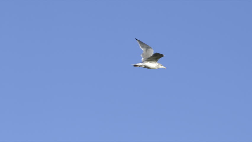
Below, we illustrate the obtained results on the RGB-image “Seagull”¹ of dimension $852\times 480$ (Fig. 4).

Fig. 4.

The $852\times 480$ image “Seagull”: original (left); and with 115 keypoints from the two scale-spaces (right).

We got the following numbers of keypoints: 45 in the first scale-space, 70 in the second scale-space, and 115 in both. It is important to emphasize that some of the keypoints can be merged, so that their total number can be reduced. However, this step requires further analysis and it is computationally expensive. Therefore, we created three different fuzzy partitions: one for each set of keypoints and calculated three different direct and inverse F-transforms using the corresponding sets of keypoints as nodes of the partition units. The quality estimates are given in Table 1.

Table 1. MSE and SSIM quality indicators

8 Conclusion

We are focused on a new fast and robust algorithm of image/signal feature extraction in the form of representative keypoints. We have contributed to this topic by showing that the use of non-traditional kernels derived from the theory of F-transforms [9] leads to simplified algorithms and comparable efficiency in the selection of keypoints. Moreover, we reduced their number and enhanced robustness. This has been shown at the theoretical and experimental levels. We also proposed a new keypoint descriptor and tested it on matching financial time series with high volatility.

References

Arrieta, A.B., et al.: Explainable artificial intelligence (XAI): concepts, taxonomies, opportunities and challenges toward responsible AI. Inf. Fusion 58, 82–115 (2020)
Elmoataz, A., Lezoray, O., Bougleux, S.: Discrete regularization on weighted graphs: a framework for image and manifold processing. IEEE Trans. Image Process. 17, 1047–1060 (2008)
Burt, P.J.: Fast filter transform for image processing. Comput. Graph. Image Process. 16, 20–51 (1981)
Klinger, A.: Pattern and search statistics. In: Proceedings of Symposium Held at the Center for Tomorrow, the Ohio State University, 14–16 June, pp. 303–337 (1971)
Koenderink, J.J.: The structure of images. Biol. Cybern. 50, 363–370 (1984)
Lindeberg, T.: Scale-space theory: a basic tool for analyzing structures at different scales. J. Appl. Stat. 21, 225–270 (1994)
Lindeberg, T.: Image matching using generalized scale-space interest points. J. Math. Imaging Vision 52(1), 3–36 (2015)
Lowe, D.G.: Distinctive image features from scale-invariant keypoints. Int. J. Comput. Vision 60(2), 91–110 (2004)
Perfilieva, I.: Fuzzy transforms: theory and applications. Fuzzy Sets Syst. 157(8), 993–1023 (2006)
Molek, V., Perfilieva, I.: Deep learning and higher degree F-transforms: interpretable kernels before and after learning. Int. J. Comput. Intell. Syst. 13(1), 1404–1414 (2020)
Perfilieva, I., Vlasanek, P.: Total variation with nonlocal FT-Laplacian for patch-based inpainting. Soft Comput. 23, 1833–1841 (2019)
Schmid, C., Mohr, R.: Local grayvalue invariants for image retrieval. IEEE Trans. Pattern Anal. Mach. Intell. 19(5), 530–535 (1997)
Witkin, A.P.: Scale-space filtering. In: Proceedings of 8th International Joint Conference on Artificial Intelligence, IJCAI 1983, vol. 2, pp. 1019–1022 (1983)
Acknowledgment
The work was supported from ERDF/ESF by the project “Centre for the development of Artificial Inteligence Methods for the Automotive Industry of the region” No. \(CZ.02.1.01/0.0/0.0/17_049/0008414\). Additional support of the grant project SGS18/PrF-MF/2021 (Ostrava University) is kindly announced.
Author information
Authors and Affiliations
Corresponding author
Editor information
Editors and Affiliations
Rights and permissions
Copyright information
© 2021 Springer Nature Switzerland AG
About this paper
Cite this paper
Perfilieva, I., Adamczyk, D. (2021). Features as Keypoints and How Fuzzy Transforms Retrieve Them. In: Rojas, I., Joya, G., Català, A. (eds) Advances in Computational Intelligence. IWANN 2021. Lecture Notes in Computer Science(), vol 12862. Springer, Cham. https://doi.org/10.1007/978-3-030-85099-9_2
Download citation
DOI: https://doi.org/10.1007/978-3-030-85099-9_2
Published:
Publisher Name: Springer, Cham
Print ISBN: 978-3-030-85098-2
Online ISBN: 978-3-030-85099-9
eBook Packages: Computer ScienceComputer Science (R0)