An Integrated Pedestrian Behavior Model Based on Extended Decision Field Theory and Social Force Model

Abstract

A novel pedestrian behavior model is proposed, which integrates (1) extended decision field theory (EDFT) for tactical level human decision-making, (2) social force model (SFM) to represent physical interactions and congestions among people and the environment, and (3) dynamic planning algorithm involving AND/OR graphs. Furthermore, SFM is enhanced with the vision of each individual, and both individual and group behaviors are considered. The proposed model is illustrated and demonstrated with a shopping mall scenario (a typical mall in the city of Tucson, AZ). Literature survey and observations have been conducted at the mall for data collection and partial validation of the proposed model. The computational environment for human-in-the-loop experiment is also conceptually developed, which will be used to collect more human data in the future. We then developed a simulation model of the considered mall using AnyLogic^® software, where each individual in the simulation executes a planning algorithm to select a destination, EDFT for choosing a direction, and extended social force model (ESFM) to adjust its velocity. Using the constructed crowd simulation model, several experiments have been conducted to test the impact of various factors (e.g. consideration of human’s vision, group shopping behavior, arrangement of stores, complexity of the model) on several metrics such as the average distance among neighboring shoppers, the movement speed of pedestrians, profit of the shopping mall, and scalability.

These keywords were added by machine and not by the authors. This process is experimental and the keywords may be updated as the learning algorithm improves.

4.1 Introduction

Human crowd dynamics is an essential factor in designing facilities involving a large crowd considering both emergency conditions (e.g. emergency evacuation from a stadium) (Helbing et al. 2005) as well as normal conditions (e.g. shopping mall) (Parisi et al. 2009). Over the past decade, several models have been developed to analyze the underlying mechanism of large-scale crowd behaviors. Xia et al. (2009) classified those models into two major categories: (1) macroscopic models focusing on extremely large crowds whose crowd behaviors are represented via a continuous flow as a whole (as opposed to individualized behaviors) (Gaskell and Benewick 1987; Xia et al. 2009) and (2) microscopic models for studying relatively small crowds whose behaviors emerge from interactions among individuals [e.g. cellular automaton model (Blue and Adler 2001); social force model (SFM) (Helbing et al. 2000); and lattice-gas model (Muramatsu et al. 1999)]. As macroscopic models focus on the continuous flow of crowd as opposed to highly variant, individualized behaviors, they have been mostly applied to the crowd behaviors under competitive situations (e.g. emergency evacuation from a building resulting in a highly dense crowd), where panicking individuals are usually driven by their instincts before every movement and tend to show maladaptive and relentless mass behavior (Helbing 2000). On the other hand, microscopic models pay more attention to individual differences (e.g. preferences, destinations, and tightness in schedule). As our interest in this work is on pedestrian behaviors in a shopping mall (under a normal situation), we will focus on microscopic models.

The SFM introduced by Helbing (2000) is a widely used microscopic model, used for various applications, such as prediction and analysis of congestion, assessment of building or urban layouts and planning of evacuation strategies (Helbing 2005; Moussaïd et al. 2009). Since the original SFM, several researchers have proposed variations or an extended version of it. For example, Hu et al. (2009) extended the model by taking into account the anisotropic characteristic of pedestrian movement in terms of pedestrian vision. Similarly, Parisi et al. (2009) applied the concept of respect area to the original model, which enabled to reproduce the experimental data (e.g. specific flow rates and fundamental diagram of pedestrian flows) for normal conditions.

While extensive works have been performed to enhance the original SFM with various other aspects, limited research works are available in the literature that integrate the human decision-making aspect with SFMs. This has motivated our research, the goal of which is to develop a crowd behavior modelthat integrates (1) tactical level human decision-making, (2) operational-level congestions among people, and (3) detailed-level perceptions (e.g. vision) of individuals. In particular, in the proposed crowd behavior model, decisions on selecting one from alternatives (e.g. destinations and movement directions) are made based on the extended decision field theory (EDFT; Lee et al. 2008), and the physical interactions are represented by the extended social force model (ESFM), which is proposed in this research enhanced with the vision of each person. In addition, pedestrian group behaviors as well as their communications are also explicitly considered in this work. The proposed model is illustrated and demonstrated with a shopping mall scenario providing us with various environmental conditions (e.g. different kinds of shops, obstacles, promotions on the shops) and population variations (e.g. gender, age, preference, schedule, and grouping). Consideration of a rich set of attributes for the environment as well as people will allow us to mimic a real shopping mall environment closely. In particular, the scenario has been built based on the shopping corridor of Tucson Mall (the largest mall in the city of Tucson, AZ). To this end, we have developed a simulation model of the considered shopping mall using AnyLogic^® software, where each individual in the simulation executes (1) EDFT (see Sect. 4.2.2), (2) ESFM (see Sect. 4.2.1), and (3) dynamic shopping planning (see Sect. 4.3.4). Using the constructed crowd simulation model, several experiments have been conducted for various purposes, such as (1) to test the impact of the consideration of human vision into SFM on the average distance among neighboring shoppers and the movement speed of pedestrians, (2) test the impact of the number of planned and unplanned shoppers on the profit of the considered shopping mall under low and high density cases, (3) test the impact of group shopping behavior on the profit of the considered shopping mall, (4) test the impact of arrangement of stores in the considered shopping mall on their profit score, and (5) demonstrate the scalability of the proposed model for complex scenarios. Observations have been conducted at Tucson Mall for partial validation of the proposed model and simulations.

The remainder of this paper is organized as follows. In Sect. 4.2, we describe the proposed pedestrian behavior model, its submodules, and techniques employed for the submodules. Section 4.3 describes the development of crowd simulation models based on the proposed behavior model, and computational environments for human-in-the-loop experiments. Section 4.4 discusses five experiments conducted using the developed crowd simulation models. Finally, Sects. 4.5 and 4.6 discuss the conclusions and future work.

4.2 Proposed Integrated Pedestrian Behavior Model

The proposed pedestrian behavior model is based on the integration of extended Decision-Field-Theory (for tactical-level decisions such as selecting a destination or a movement direction during shopping) and extended SFM for dynamic congestions among shoppers and the environment (e.g. walls and obstacles). Each of them is discussed in detail below.

4.2.1 Extended Social Force Model

Helbing (2000) has proposed an SFM, where the motives and impacts to a pedestrian crowd are represented by a combination of physical and psychological forces (which are translated into the acceleration equation). Equation 4.1 depicts the formulation of changing velocity at time t, where a pedestrian i’s velocity v _i is determined by his/her desired speed v ⁰ _i (t) and desired direction e ⁰ _i (t) as well as interactions with other individuals and obstacles.

$$ m_{i} \frac{{dv_{i} }}{dt} = m_{i} \frac{{v_{i}^{0} (t)e_{i}^{0} (t) - v_{i} (t)}}{{\tau_{i} }} + \sum\limits_{j( \ne i)} {f_{ij} } + \sum\limits_{W} {f_{iW} } $$

(4.1)

where m is the pedestrian mass, τ _i is a time constant related to the relaxation time of the particle to achieve v _i .

The first term on the right-hand side of Eq. 4.1 represents the impact from the pedestrian’s self-consciousness while f _ij and f _iW illustrate interaction forces from pedestrian j and the wall W, respectively. The pedestrians try to keep a velocity-dependent distance from other people and the walls so as to construct a comfortable zone for themselves. The interaction force consists of a socio-psychological force f ^psy _ij resulting from the distance between each other, and a physical force f ^phy _ij inspired by counteracting body compression and sliding friction. The total force exerted by pedestrian j to pedestrian i is calculated as below:

$$ f_{ij} = f_{ij}^{\text{psy}} + f_{ij}^{\text{phy}} $$

(4.2)

$$ f_{ij}^{\text{psy}} = A_{i} \exp \left( {\frac{{r_{ij} - d_{ij} }}{{B_{i} }}} \right){\user2{n}}_{ij} $$

(4.3)

where A and B are constants that describe the strength and range of psychological interaction, r _ij is the sum of radii of pedestrian i and j, dij is the distance between i and j, n _ij is the unit vector pointing from j to i.

$$ f_{ij}^{\text{phy}} = {\text{k}}g(r_{ij} - d_{ij} ){\user2{n}}_{ij} + {{\upkappa}}g(r_{ij} - d_{ij} )\Updelta v_{ji}^{t} {\user2{t}}_{ij} $$

(4.4)

where k and κ are the normal and tangential elastic restorative constants, t _ij is tangential unit vector perpendicular to n _ij , v ^t _ij is the tangential projection of the relative velocity seen from pedestrian j (v _ij = v _i − v _j ), and g is 1 if d _ij > r _ij and 0 otherwise.

While the original SFM (Helbing 2000) discussed above has been extensively applied to pedestrian behavior modeling, there exist two improvement opportunities when applying to a real-life human behavior. First, the original SFC computes a force impact between every pair of agents in the environment. In other words, there will be a force even between agents who are significantly far away from each other, which is not realistic. Second, the social force between agents is always positive implying that all agents are psychologically against each other. However, this is not the case for friends or family members, who usually stay close to each other while moving (shopping in our case) under a nonemergency condition. To address these two problems, we extended the original SFC. Details of each modification will be discussed in Sects. 4.2.1.2 and 4.2.1.3.

4.2.1.1 Connection Range Impact on Social Force Model

Experimental investigations have demonstrated the self-organization phenomenon to be a typical characteristic of pedestrians. With the help of technologies like video tracing, researchers have further found that self-organization is caused by collision avoidance behavior. In other words, pedestrians tend to keep a suitable distance from others to avoid bumping into one another (Ma et al. 2010). Therefore, in this work we define a connection range, CR, for each agent in the environment. Before applying the force (see Eq. 4.2) between two agents, ESFM will evaluate the distance, d _ij , between them first and compare it with the connection range. Only if d _ij < CR, are these two agents connected and have a force affecting their movement (see Eq. 4.5). However, there is an exception for the group members, which will be discussed in Sect. 4.4.1. Considering the radius of agent r _i in the range between 0.25 and 0.35 m (Helbing et al. 2000), we have chosen CR as 5 m in this work so that pedestrians could get more information from their surroundings (Ma et al. 2010).

$$d_{ij} \left\{\begin{gathered} > {\rm CR}\,{\text{agent}}\,i\,{\text{and}}\,j\,{\text{are not connected}} \hfill \\ \leq {\rm CR}\,{\text{agent}}\,i\,{\text{and}}\,j\,{\text{are connected}} \hfill \\ \end{gathered} \right.$$

(4.5)

4.2.1.2 Psychological Attraction Between Group Members

Pedestrian populations in the shopping mall (case study in this research) can be categorized into two types: individual shoppers and group shoppers (see Sect. 4.3 for more details about the considered scenario). Among individual shoppers or shoppers from different groups, a psychological force in the original SFC is applicable to keep a comfort distance between them. However, for shoppers belonging to the same group, the psychological force will prohibit them from staying close to each other. Therefore, we propose a modification of the psychological force for members of the same group (see Sect. 4.4.1 for more details), where an intimate factor I _ij (see Eq. 4.6) is multiplied with the psychological force (see Eq. 4.3). The main idea is that a positive psychological force is applicable for people belonging to different groups while a negative psychological force is applicable for people belonging to the same group (Helbing 2005).

$$ I_{ij}=\left\{\begin{array}{ll}1,&i\,{\text{and}}\,j\,{\text{are group members}}\\ -1,&{\text{otherwise}} \end{array} \right.$$

(4.6)

4.2.1.3 Pedestrians’ Reactions According to Their Visions

In the original SFM, obstacles located at the same distance (without considering the concept of vision or sight) from a pedestrian enforce the equal psychological force on him/her. In a real shopping environment, however, people usually pay more attention to objects within their vision than to those out of their sight. To resolve this problem, we incorporate this concept of vision by defining a visible area for each agent in this work. From the view of an agent, only neighbors in his visible area could affect his movement with psychological force. Neighbors behind his back (out of vision) may provide influence only via a physical force (e.g. contact). In our proposed model, a visible area (range) is defined with a half circle in front of each pedestrian (±90 degree angle from the pedestrian’s current moving direction) (see Figs. 4.1, 4.2). The vision formula is given in Eq. 4.7, where φ _ij (t) is the angle between direction e _i (t) and normalized vector n _ij (t). Withφ _ij (t) > 90°, cos (φ _ij (t)) (<0) is rounded up to 0, whileφ _ij < 90° will round cos(φ _ij (t)) (≥0) up to 1. Based on this visible area, a modified social force exerted from pedestrian j on pedestrian i is given in Eq. 4.8.

$$ \cos (\varphi_{ij} (t)) = \frac{{\user2{n}_{ij} (t)\user2{e}_{i} (t)}}{{\left\| {\user2{n}_{ij} (t)} \right\|\left\| {\user2{e}_{i} (t)} \right\|}} $$

(4.7)

$$ f_{ij}^{\text{psy}} = A_{i} \exp \left( {\frac{{r_{ij} - d_{ij} }}{{B_{i} }}} \right){\user2{n}}_{ij} I_{ij} \left\lceil {\cos (\varphi_{ij} (t))} \right\rceil $$

(4.8)

Fig. 4.1

Sequence diagram of components of the proposed pedestrian behavior model

Fig. 4.2

Visible area for each agent

4.2.2 Incorporating EDFT into the Pedestrian Model

It is generally agreed that decision making about walking trips takes place simultaneously at two or more levels: (1) decisions about basic strategy of the trip, (2) route choice, and (3) local spatial behavior considering velocity, trajectory, stops, and attention direction (Zacharias 2005). In this work, it is assumed that a basic strategy (which shops to stop by) and a route choice (in what sequence) are fixed for each individual. Therefore, pedestrian’s decisions, of interest to us, are focused on changing their movement directions. Since pedestrians adjust their actual direction from time to time due to the interaction force, the EDFT is employed in this work to mimic this dynamic human decision deliberation process.

Decision Field Theory (DFT) is a psychology-based model and has been widely used for mimicking human deliberation process in making decisions under uncertainty (Busemeyer and Diederich 2002; Busemeyer and Townsend 1993). Lee et al. (2008) extended the original DFT to cope with a dynamically changing environment, where a Bayesian Belief Network (BBN) was used to infer human decision attributes under the dynamically changing environment. In the shopping mall scenario considered in this research, the environmental conditions (e.g. crowd density and destinations) change dynamically for individuals. Therefore, we integrate the EDFT into our proposed pedestrian model to better mimic pedestrians’ deliberation on direction changes. Our EDFT is able to model (1) the change of evaluation on the options and (2) the change of human attention along with the dynamically changing environment. The formulation of EDFT is given in Eq. 4.9, which illustrates the dynamic evolution of preferences P among options during the deliberation time h.

$$ P(t + h) = {\text{SP}}(t) + {\text{CM}}(t + h)W(t + h) $$

(4.9)

In our work, pedestrians change their movement direction according to the environment around them, for example, the increase/decrease of crowd density or the position of their next destination. Definitions of the main elements of EDFT are explained below:

• M(t) is the value matrix (n × m matrix, where each n option has m attributes) representing the subjective perceptions of a decision-maker by M(i, j). In our case (choosing a direction), a 6 × 2 matrix (see Eq. 4.10) is used, where pedestrians have six options (see Fig. 4.3), and each direction corresponds with two attributes (crowd density and destination) that affect their choice. If the next destination is within direction i, the entry value Des _i (t) is 0.5; otherwise, it is 0.1. To decide whether a destination is within a particular direction, n_iD to denote a vector from pedestrian i to the destination. If the angle between n_iD and the direction is ≤22.5°, we claim that the destination is in this direction. Thus, the value matrix M has a dynamic representation as shown in Eq. 4.10, and its values change whenever the underlying conditions change.

  $$ M(t) = \left[ {\begin{array}{*{20}c} {{\text{Den}}_{F} (t)} \\ {{\text{Den}}_{LF} (t)} \\ {{\text{Den}}_{RF} (t)} \\ \begin{gathered} {\text{Den}}_{L} (t) \\ {\text{Den}}_{R} (t) \\ {\text{Den}}_{B} (t) \\ \end{gathered} \\ \end{array} \begin{array}{*{20}c} {{\text{Des}}_{F} (t)} \\ {{\text{Des}}_{LF} (t)} \\ {{\text{Des}}_{RF} (t)} \\ \begin{gathered} {\text{Des}}_{L} (t) \\ {\text{Des}}_{R} (t) \\ {\text{Des}}_{B} (t) \\ \end{gathered} \\ \end{array} } \right] $$

  (4.10)

  Fig. 4.3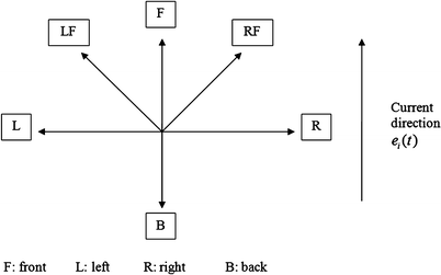

  

  Potential directions for each decision making

  where

  $$ {\text{Des}}_{i} (t) = \left\{ \begin{gathered} 0.5,{\text{ next destination is in direction }}i \\ 0.1\,,\,{\text{otherwise}} \hfill \\ \end{gathered} \right. $$

  (4.11)
  $$ {\text{Den}}_{i} (t) = \left\{ \begin{aligned} & 0.2,\quad{\text{ if }}{\text{cd}}_{i} (t) < 5 \hfill \\ & 0. 4 , \quad{\text{ if }}5 \leq {\text{cd}}_{i} (t) < 15 \\ & 0. 6 ,\quad {\text{ otherwise}} \hfill \\ \end{aligned} \right.$$

  (4.12)

  W(t) is a weight vector allocating the portion of human attention to each column j (attribute) of M through W(j, 1), which is the only dynamically changing element in the original DFT (Busemeyer and Townsend 1993). In the shopping mall environment, it is assumed that pedestrians intend to arrive at their destination as soon as possible. However, when the environment is really crowded, they tend to put more weight on the impact of crowd density. Equations 4.12 and 4.13 depict W(t) used in the considered shopping mall scenario, where cd _i (t) denotes the crowd density.

  $$ W(1,1) = \left\{ \begin{gathered} \left[ {0.2,0.3} \right]^{T} ,\quad{\text{ if }}{\text{cd}}_{i} (t) < 5 \hfill \\ [0.25,0.6]^{T} , \quad\text{if} \, 5 \le {\text{cd}}_{i} (t) < 15 \hfill \\ [0.4,0.6]^{T} ,\quad{\text{ otherwise}} \hfill \\ \end{gathered} \right.$$

  (4.13)
  $$ W(1,2) = 1 - W(1,1) $$

  (4.14)

• S demonstrates the stability of preference to each option by its structure. The diagonal elements of S represent the memory from the previous preference state while off-diagonal elements give the inhibitory interactions among competing options. Here, it is assumed that the same amounts of memory and interaction effects are given to the options: (1) matrix S is assumed to be symmetric and (2) diagonal elements of S are assumed to have the same value. Moreover, all eigenvalues λ _i of S are >1 in magnitude to make the linear system stable (|λ _i | < 1). Besides, from Fig. 4.3, we can see larger interactions between directions within 45° than those in 90 or larger degrees. Considering this, we have defined S matrix (see Eq. 4.15).

• C is the contrast matrix comparing the weighted evaluation of each option, MW(t). In our case, each option is evaluated independently, thus C tends to be I (identity matrix). Given the aforementioned elements and our six-option scenario, the corresponding DFT formula, as defined in Eq. 4.9, is described in Eq. 4.15.

  $$ \left( {\begin{array}{ll} {p_{1} (t + h)} \\ {p_{2} (t + h)} \\ {p_{3} (t + h)} \\ \begin{gathered} p_{4} (t + h) \hfill \\ p_{5} (t + h) \hfill \\ p_{6} (t + h) \hfill \\ \end{gathered} \\ \end{array} } \right) = \left( {\begin{array}{ll} {0.9} \\ { - 0.6} \\ { -0.6} \\ \begin{gathered} -0.4 \hfill \\ - 0.4 \hfill \\ - 0.1 \hfill \\ \end{gathered} \\ \end{array} \begin{array}{ll} { - 0.6} \\ {0.9} \\ {- 0.4} \\ \begin{gathered} - 0.6 \hfill \\ -0.2 \hfill \\ - 0.6 \hfill \\ \end{gathered} \\ \end{array} \begin{array}{ll} { -0.6} \\ { - 0.4} \\ {0.9} \\ \begin{gathered} - 0.2 \hfill \\- 0.2 \hfill \\ -0.2 \hfill \\ \end{gathered} \\ \end{array} \begin{array}{ll} { - 0.4} \\ { - 0.6} \\ { - 0.2} \\ \begin{gathered} 0.9 \hfill \\ - 0.1 \hfill \\ - 0.4 \hfill \\ \end{gathered} \\ \end{array} \begin{array}{ll} { -0.4} \\ { - 0.2} \\ { - 0.2} \\ \begin{gathered} - 0.1 \hfill \\ 0.9 \hfill \\ - 0.4 \hfill \\ \end{gathered} \\ \end{array} \begin{array}{ll} { - 0.1} \\ { - 0.6} \\ { - 0.2} \\ \begin{gathered}- 0.4 \hfill \\ - 0.4 \hfill \\ 0.9 \hfill \\ \end{gathered} \\ \end{array} } \right)\left( {\begin{array}{ll} {p_{1} (t)} \\ {p_{2} (t)} \\ {p_{3} (t)} \\ \begin{gathered} p_{4} (t) \hfill \\ p_{5} (t) \hfill \\ p_{6} (t) \hfill \\ \end{gathered} \\ \end{array} } \right) + \left( {\begin{array}{ll} 1 \\ 0 \\ 0 \\ \begin{gathered} 0 \hfill \\ 0 \hfill \\ 0 \hfill \\ \end{gathered} \\ \end{array} \begin{array}{ll} 0 \\ 1 \\ 0 \\ \begin{gathered} 0 \hfill \\ 0 \hfill \\ 0 \hfill \\ \end{gathered} \\ \end{array} \begin{array}{ll} 0 \\ 0 \\ 1 \\ \begin{gathered} 0 \hfill \\ 0 \hfill \\ 0 \hfill \\ \end{gathered} \\ \end{array} \begin{array}{ll} 0 \\ 0 \\ 0 \\ \begin{gathered} 1 \hfill \\ 0 \hfill \\ 0 \hfill \\ \end{gathered} \\ \end{array} \begin{array}{ll} 0 \\ 0 \\ 0 \\ \begin{gathered} 0 \hfill \\ 1 \hfill \\ 0 \hfill \\ \end{gathered} \\ \end{array} \begin{array}{ll} 0 \\ 0 \\ 0 \\ \begin{gathered} 0 \hfill \\ 0 \hfill \\ 1 \hfill \\ \end{gathered} \\ \end{array} } \right)\left( {\begin{array}{ll} {M_{11} (t + h)} \\ {M_{21} (t + h)} \\ {M_{31} (t + h)} \\ \begin{gathered} M_{41} (t + h) \hfill \\ M_{51} (t + h) \hfill \\ M_{61} (t + h) \hfill \\ \end{gathered} \\ \end{array} \begin{array}{ll} {M_{12} (t + h)} \\ {M_{22} (t + h)} \\ {M_{32} (t + h)} \\ \begin{gathered} M_{42} (t + h) \hfill \\ M_{52} (t + h) \hfill \\ M_{62} (t + h) \hfill \\ \end{gathered} \\ \end{array} } \right)\left( {\begin{array}{ll} {W_{11} (t + h)} \\ {W_{21} (t + h)} \\ \end{array} } \right) $$

  (4.15)

4.3 Development of Agent-Based Simulation Based on Proposed Pedestrian Model

This section describes the development of a crowd simulation model for a shopping mall scenario, where behaviors of individual shoppers are based on the proposed, integrated pedestrian behavior model (see Sect. 4.2). We employed a two-layer modeling principle (Hamgami and Hirata 2003) in the development of the crowd simulation model to reduce the complexity of the modeling process, where agents and the environment they interact with are modeled separately in two conceptual layers. The interactions between agents and the environment are analogous to how humans behave in the real world. Agents evaluate the surroundings and try to make optimal decisions so as to achieve their intentions. Figure 4.4 depicts a state chart for shoppers, which contains different states in which shoppers will be in and their transitions. More details about each state and simulation models will be discussed in the following sections.

Fig. 4.4

State charts for the shopper’s behavior

4.3.1 Shopping Mall (Case Study) and Customer Classifications

A shopping mall scenario has been designed, and its simulation implemented using AnyLogic^® 6.4 agent-based simulation software. The considered scenario covers eight shops of four different types: three clothing shops, two sports shops, two beauty shops, and one candy shop. Each shop has its own ID as listed in Table 4.1. Each type of shop has its target customers. For instance, female customers may be more interested in beauty shops while males may be more interested in sports shops. In this work, to enhance the validity and realism of the constructed simulation model, we have categorized customers in multiple ways. Table 4.2 depicts multiple categories of customers considered in this work. First, customers are tagged with three agent types based on their gender and age: (1) female adult, (2) male adult, and (3) child. In this work, the agent type is based on the ratios of sex and age of the Tucson population (http://www.maps-n-stats.com/). Therefore, agent type is determined based on the discrete, empirical statistical distribution shown in Eq. 4.16.

$$ P_{{agent\,type}} = \left\{ \begin{gathered} {[0,0.4]},{\text{ agent type is female adult}} \hfill \\ (0.4,0.8],{\text{ agent type is male adult}} \hfill \\ (0.8,1.0],{\text{ agent type is child}} \hfill \\ \end{gathered} \right. $$

(4.16)

Table 4.1 Shop list in the simulation scenario

Table 4.2 Agent categorizations

Besides utilitarian-oriented shopping, there also exists window shopping orientation and recreational shopping. Therefore, based on their shopping style, customers are categorized into planned shoppers (people who go to the mall with specific shopping plan) and unplanned shoppers (who do not have a specific shopping plan). Upon arriving at the mall, planned shoppers already have in mind which shops they will visit. Planned shoppers are further partitioned into group shoppers (those who do shopping with friends or family members) and individual shoppers. In this work, it is assumed that all the unplanned shoppers are individual shoppers. By combining agent type with other categorizations (e.g. planned vs. unplanned shoppers; individual verses group shoppers), we can enhance the flexibility of pedestrians’ behaviors as well as their adaptability to the environment.

4.3.2 Algorithm for Movement of Pedestrians

In this section, the algorithm for movement of pedestrians is discussed in detail. Figure 4.5 depicts a flowchart of the movement algorithm. As discussed in Sect. 4.2.2, a desired destination is used as part of input M for EDFT during the decision deliberation on directions. For the planned shoppers, a potential destination is obtained from their shopping plans. On the other side, unplanned shoppers normally set the closest shop as their potential destination. In this work, an attribute (crowdedness threshold) is defined to represent the largest number of people that each shopper could accept to shop with in the same store. Before a shopper enters his/her planned destination (shop), he/she will evaluate it based on several criteria such as their interest level, shop’s attraction level, and crowdedness level, and confirm the desired destination based on their evaluations. More details about evaluation of the destination will be illustrated in Sects. 4.3.3 and 4.3.4 for unplanned and planned shoppers, respectively. As soon as an agent (shopper) comes up with a desired destination, he/she utilizes EDFT to determine their next moving direction. To implement/compute EDFT, a Java Matrix Package (JAMA) has been embedded into our simulator (Anylogic model). Then, by calculating the physical and social forces based on the surroundings along the moving direction, each agent adjusts its velocity in SFM (see Eq. 4.1).

Fig. 4.5

Pedestrian moving algorithm

4.3.3 Destination Confirmation Algorithm for Unplanned Shoppers

As mentioned earlier, unplanned shoppers wander around the shopping mall, without knowing in advance which shop they will visit. When they pass by a shop, they will set it as a potential destination if the shop’s crowdedness level is below their threshold. Then, they evaluate the shop based on their personal interest and the shop’s attraction level by Eq. 4.17. Based on this evaluation, the potential destination may become a confirmed destination. For instance, a male, unplanned shopper who is more interested in sports shoes than cosmetics may enter a sports shop but not a beauty shop when he passes by one of them. However, if the beauty shop has a special promotion (e.g. big sale), he may still visit the shop. Equation 4.17 depicts a probability function on whether unplanned shoppers enter a shop or not.

$$ P_{iw} = \alpha I_{iw} + \beta A_{iw} $$

(4.17)

I _iw denotes the interest level of agent i for shop w, while A _iw describes the attraction level of shop w towards agent i. Constants α and β are the weight values assigned to the interest level and attraction level, respectively. Both variables (I _iw , A _iw ) and constants (α, β) range from 0 to 1. In our model, we give the same weight to I _iw and A _iw by setting α = β = 1. Therefore, in the normalization step, the value obtained for P _iw is divided by 2 in order to obtain its normalized value. Here, we assume that P _iw > 0.5 indicates that agent i is definitely attracted by shop w and will enter this shop.

4.3.4 Planning Algorithm for Planned Shoppers

Planned shoppers obtain their potential destinations based on their shopping plan, and evaluate them in the same way as unplanned shoppers (see Sect. 4.3.3). If the potential destination does not meet one of their three criteria (interest level, shop’s attraction level, and shop’s crowdedness level), planned shoppers will need to decide whether they will skip the shop or move to another shop (of the same kind). This decision process is defined as plan adjustment. The following sections discuss the design of initial shopping plans and the plan adjustment algorithm for planned shoppers in greater detail.

4.3.4.1 Alternative Initial Shopping Plans for Planned Shoppers

When planned agents arrive at the entrance of the mall, they will be offered with initial shopping plans according to their characteristics (see Table 4.2). For individual planned shoppers, the plan is designed based on their agent type. For instance, female shoppers may want to visit all three clothes shops and two beauty shops if their schedule permits. Thus their initial shopping plan will include these shops. For a male shopper, a different plan will be designed according to his personal need. Table 4.3 depicts the shopping plans for individual shoppers. Plans in Table 4.3 contain alternatives in stores to visit (using OR junctions) or in the sequence of stores to visit (using AND junctions).

Table 4.3 Predefined shopping plans for individual shoppers

Based on the survey conducted by Kuruvilla et al. (2009) and observations made in the real shopping environment, we have partitioned shopping groups into three types based on their shopping interest and group members’ personal characteristics: (1) female groups consisting of female shoppers whose interests mainly focus on beauty and clothing shops; (2) mixed gender groups with both male and female members; and (3) family with-kid groups. Family groups are mixed-gendered groups that need to balance shopping interests, but they will include candy shops on their plan due to kids. For group shoppers, their shopping plans are not based only on one person’s interests, but should consider the need of all the members in the group and achieve a balance for the whole group’s interests. Taking a mixed-gender group for example, while female members may need to visit more beauty shops and males may need to visit sports shops, the group shopping plan would include both types but only one shop (less than what is preferred by each party) for each type. As another example, if there is a kid in the group (family group), adult members may have to give up one of their shops of interest (e.g. sports, clothes, or beauty) since they may need to go to the candy shop with the kid. When group shoppers enter the mall, they will be assigned with a group ID (0 ~ 8), which will indicate the group type they belong to. Table 4.4 depicts group types and the corresponding initial plans. The group frequencies vary by scenario (e.g. different ethnicity). For example, about 70% of Indian people always shop with families while the percentage is lower for American shoppers (Kuruvilla et al. 2009).

Table 4.4 Predefined shopping plans for group shoppers

As shown in Tables 4.3 and 4.4, initial shop plans contain alternatives, and one of them will need to be selected based on the current situation. Taking a female adult as an example in Table 4.3, she needs to visit shop A and shop B upon her arrival, but in any sequence. This selection is based on both her current position and the shop selection probability. If she enters the mall at area 1 in Fig. 4.8, the probability of selecting shop B is higher than that of shop A because of its proximity. In this work, we use P _sw to denote the probability that shop w will be selected by a nearby agent and Pos _k to denote the position of agent. Then the probability of selecting shop A and shop B as the first destination is given by Eqs. 4.18 , and 4.19, respectively.

$$ P_{A} = {\text{Pos}}_{2} *P_{sA} + {\text{Pos}}_{1} *(1 - P_{sB} ) $$

(4.18)

$$ P_{B} = {\text{Pos}}_{1} *P_{sB} + {\text{Pos}}_{2} *(1 - P_{sA} ) $$

(4.19)

where

$$ {\text{Pos}}_{k} = \left\{ \begin{aligned} & {1}, \quad{\text{ if an agent's entering position in area }}i; \\ & {0}, \quad{\text{otherwise}} \end{aligned} \right. $$

(4.20)

$$ P_{sA} = P_{sB} = 0.7 $$

(4.21)

4.3.4.2 Plan Adjustment for Individual Planned Shop

As described in Sect. 4.3.4, a potential destination of planned shoppers becomes a confirmed one if the shop’s crowdedness level is below their threshold. If a considered shop is too crowded, they may want to skip it and go to a next planned one or adjust their plan to visit a different shop (of the same kind). Figure 4.6 illustrates the procedure in which planned shoppers adjust their shopping plans according to dynamically changing surroundings. For individual shoppers, they evaluate a shop according to Eq. 4.17 just as unplanned shoppers do. We use P _iw to denote the probability that agent i would like to stop by shop w. If P _iw is larger than 0.5, they will choose to visit a similar shop instead. Otherwise, they will skip the shop and set a next planned shop as the potential destination.

Fig. 4.6

Plan adjustment algorithm against dynamic situations

4.4 Experiments and Results

Using the crowd simulation model constructed based on the proposed pedestrian model and data (survey and observations), we have conducted several experiments for various purposes, such as (1) to test the impact of consideration of human’s vision into SFM on the average distance among neighboring shoppers and the movement speed of pedestrians, (2) test the impact of the number of planned and unplanned shoppers on the profit of the considered shopping mall under low and high density cases, (3) test the impact of group shopping behavior on the profit of the considered shopping mall, and (4) test the impact of arrangement of stores in the considered shopping mall on their profit score. Also, we tested the scalability of the proposed model by increasing the number of agents in the simulation. The detailed design of each experiment, results, and analyses are described in the following sections.

4.4.1 Significance of Consideration of Vision in Social Force Model

The goal of this experiment is to test the significance of consideration of human’s vision into SFM, which is part of the proposed pedestrian behavior model in this work. As mentioned in Sect. 4.2, one of the group characteristics is the positive social force among the group members. Unlike individual and group shoppers belonging to different groups, group members of the same group stay close to each other and move together. In Sect. 4.2.1.1, a concept of connection range (CR) was discussed for the social force between agents except the group members. The exception for the group members is that even if two group members are out of their connection range, there is still a psychological force f ^psy between them in order to reduce the distance between them. Once they get closer and are within the connection range, a physical force f ^phy begins working to avoid any friction or collision between them. Figure 4.7 depicts the forces between group members from group member i’s view. Equation 4.22 depicts the resultant force function for the group members.

$${f_{ij}} = \left\{\begin{array}{ll} {f_{ij}^{psy}}+{f_{ij}^{phy}}, &{d_{ij}} \leq CR\\ {f_{ij}^{psy}}, &{d_{ij}} >CR\end{array} \right.$$

(4.22)

Fig. 4.7

Force execution between group members (from group member i’s view)

By considering the human vision in SFM, pedestrians will have a psychological force against only those neighbors in front of them and adjust their speed consequently. In this case, their resistance force is reduced; therefore, they are hypothesized to move faster. Then we do the Student’s t test with alternative hypothesis H ₁ and null hypothesis H ₀ stated as below:

H ₁ :

Pedestrians will tend to move faster when vision is considered

H ₀ :

Pedestrians will not move faster when vision is considered

Figure 4.8 depicts a snapshot of the shopping mall simulator that we have developed, where 100 pedestrians are moving along the hallway towards the exit. This experiment was designed in a way that pedestrians do not visit any shop. Therefore, it allows us to test the significance of consideration of human vision into SFM in a general case, where the average speed of pedestrians is used as a metric. Experiments have been conducted with 30,100, and 1,000 pedestrians to compare average speeds between models with and without consideration of human vision. Statistics shown in Table 4.5 are based on 16 samples collected every 10 s in each case. By using student’s t testing with equal sample sizes and unequal variance, we obtained p-value <0.001 which accepts our hypothesis. The experimental results reveal that our intuition on faster movement of pedestrians when we consider human vision is correct regardless of the crowd density. Therefore, consideration of human vision into SFM has been found to be significant (Fig. 4.9).

Fig. 4.8

Snapshot of a shopping mall simulation with 100 participants

Table 4.5 Statistics of Student’s t testing on the significance of vision in SFM

Fig. 4.9

Average speed of pedestrians in SFM with and without considering of vision

4.4.2 Impact of Unplanned Shoppers on the Number of Visits to Shops

The goal of this experiment is to analyze the impact of the number of unplanned shoppers on the number of visits to the shops (and therefore profit of the shopping mall) during the same time period. As mentioned in Sect. 4.3.3, shoppers (planned and unplanned) will evaluate the crowdedness of a shop before entering it. Equation 4.23 depicts the probabilities that planned and unplanned shoppers will purchase items used in this experiment. Equation 4.24 depicts the profit of shop w, where m denotes the minimum crowdedness threshold of the shopper in the shop. If shops are mostly filled with unplanned shoppers, they may lose the opportunity to attract planned shoppers whose probability of purchasing is higher, reducing the profit of the shop. For unplanned shoppers, we assumed equal chances for them to make a purchase or not while visiting a shop. Many previous studies (Zhuang et al. 2006; Babin et al. 1994; Batra and Ahtola 1991; Baumann et al. 1981) found that the buying intention tends to increase shoppers’ buying of non-food products such as clothes; we give higher purchase probability to planned shoppers.

$${\text{P{r}}}_{i} ({\text{purchase}})\left\{\begin{array}{ll} < 0.5, {\text{ is a planned shopper}} \hfill \\ = 0.5, {\text{ is an unplanned shopper}} \hfill \\ \end{array} \right. $$

(4.23)

$$ {\text{ProScore}}_{w} = \sum\limits_{i}^{m} {\text{P{r}}_{i} } ({\text{purchase}}) $$

(4.24)

The first experiment has been conducted with a high density envrionment, where the total profit score of the mall for 100 min is compared under three different conditions: (1) 54 planned shoppers and 76 unplanned shoppers in the mall, (2) 57 planned shoppers and 117 unplanned shoppers in the mall, and (3) 96 planned shoppers and 78 unplanned shoppers in the mall. By setting the purchasing probability of planned shoppers as 0.6 and 0.8 repectively, we could see from Figs. 4.10 and 4.11 the impact of shoppers’ buying intention on the mall’s profit gaining. As depicted in Figs 4.11a and b, cases 1 and 2 indicate that the profit score does not increase greatly when about 40 additional unplanned shoppers are in the mall. Figure 4.11c, however, demonstrates that 40 additional planned shoppers in the mall increases the profit score from 125 to nearly 250. When we decrease Pr(purchase) from 0.8 to 0.6, the profit does not increase much by adding either more unplanned or more planned shoppers. Besides, the profit from planned shoppers is almost the same as that from unplanned shoppers. In other words, the higher the buying intention, the more profit the mall will gain. Therefore, operational strategies such as promotion should target at increasing shoppers’ buying intention.

Fig. 4.10

Results for testing the impact of unplanned shoppers on the profit of the mall under a high density case [Pr(purchase) = 0.8]

Fig. 4.11

Results for testing the impact of unplanned shoppers on the profit of the mall under high density case [Pr(purchase) = 0.6]

Next, an experiment involving a low density environment has been also conducted with 29 planned shoppers and 39 planned shoppers (See Fig. 4.12a), where planned shoppers’ purchase probability is 0.8. By adding 20 more unplanned shoppers (see Fig. 4.12b) and planned shoppers (see Fig. 4.12c) into the mall, respectively, smaller differences are observed compared with the case with higher density environment. According to our experiments, it has been found that the impact of the number of unplanned shoppers on the profit of the mall is more obvious when the mall is more crowded (e.g. during holidays or weekends). It is believed that this finding (and more detailed simulation results) would be very useful for the shopping mall management when they design promotion and/or advertisement policies during the regular as well as busy seasons.

Fig. 4.12

Results for testing the impact of unplanned shoppers on the profit of the mall under a low density case [Pr(purchase) = 0.8]

4.4.3 Impact of Group Shopping Behavior on the Profit of Mall

As described in Sect. 4.3.4.2, individual shoppers would skip a planned shop or go to an alternative one (of the same type) if the crowdedness level in that shop is above their threshold. They make these decisions only based on their interests and how the shop attracts them (e.g. promotion). However, when a member in a group wants to skip a planned shop or go to an alternative shop, he/she needs to communicate (discuss) with all the other group members first and follow the group’s final decision (which may accept or reject his/her proposal). Therefore, the chance that group shoppers skip or alter a shop is lower than that of individual shoppers. The goal of this experiment is to test our intuition that the shopping mall will gain more profit as the percentage of group shoppers increases. Figure 4.13a depicts the experimental results for the case with 48 individual planned shoppers, 50 group planned shoppers, and 89 unplanned shoppers. Here, the ratio between the group shoppers to the individual shoppers is about 1. Figure 4.13b depicts the experimental results for the case, where the number of unplanned shoppers remains unchanged, the number of group shoppers is increased to 70, and the number of individual shoppers is reduced to 34. It is clearly shown in Fig. 4.13b that the profit score increases as the percentage of the group shoppers increases.

Fig. 4.13

Results for testing the impact of group shopping behavior on the profit of the mall

4.4.4 Arrangement of Stores

An empirical study conducted by Zhuang et al. (2006) demonstrated that the number of stores visited has a negative impact on shoppers’ purchase. We observe that similar shops are usually located near to each other in many large shopping malls such as Dillards and Macy’s. The goal of this experiment is to test the impact of the arrangement of stores in the considered shopping mall on their profit score. Two different configurations have been considered: (1) same-type shops are placed far from each other (see Fig. 4.14) and (2) same-type shops are placed close to each other (see Fig. 4.15). Experimental results reveal that the shopping mall gains a higher profit for the second configuration. One possible reason could be that people are more likely to make a purchase in a similar store nearby if their original planned destination is crowded. To validate this conjecture, further study such as survey on shoppers will be valuable.

Fig. 4.14

Configuration 1: placement of similar stores far from each other

Fig. 4.15

Configuration 2: placement of similar stores together

4.4.5 Scalability and Computational Aspects

In this research, several efforts have been made to enhance the validity of the crowd simulation model for the considered shopping mall, such as (1) adopting EDFT to mimic decision deliberation of each individual pedestrian (at each point to choose a next direction), (2) incorporation of explicit group communications, and (3) consideration of human’s vision into pedestrian’s movement (SFM). However, it is expected that these additions will result in longer simulation execution times. The goal of this experiment is to test the scalability of the proposed, integrated pedestrian behavior model in terms of computational requirements. By increasing the number of agents involved in the simulation, we have evaluated the simulation execution times. As shown in Fig. 4.16, simulation execution times increase nearly linearly when the number of agents increases. Therefore, it is believed that our modeling approach is extensible to more complex situations without involving significant increase in the computational time.

Fig. 4.16

Simulation execution times with increase in the number of agents

4.5 Conclusion

The integrated pedestrian model proposed in this chapter has allowed us to develop a more realistic simulation of pedestrian behaviors at a shopping mall. In particular, consideration of the vision of each individual allowed us to mimic physical and psychological interactions among the people and the environment more realistically. Similarly, consideration of the EDFT (based on the psychological principle) allowed us to represent the human decision deliberation process, where economic approaches based on expected values are not always applicable. In addition, consideration of a rich set of attributes for the environment (different kind of shops, obstacles, promotions on the shops) as well as people (e.g. gender, age, preference, schedule, and grouping) has allowed us to mimic a real shopping mall environment closely. A crowd simulation model constructed based on the proposed pedestrian model and data (survey and observations) has been used to conduct several experiments. Our experimental results revealed several interesting findings such as (1) consideration of human vision into SFM (part of the contribution in this work) is found to be significant, (2) impact of shoppers’ buying intention on the profit of the mall, especially when the mall is crowded (e.g. during holidays or weekends), (3) the profit score largely increases as the percentage of the group shoppers increases, and (4) the shopping mall gains a higher profit if similar-type shops are placed close to each other. It is believed that many of these findings (and more detailed simulation results) would be very useful for the shopping mall management when they make strategic decisions (e.g. layout design and arrangement of stores) as well as operational decisions (e.g. promotion and/or advertisement policies during the regular as well as busy seasons).

4.6 Future Work

Currently, the dynamic planning algorithm is based on a rather simple probability, but our future work will employ the extended decision field theory for shopping path planning according to the dynamically changing environment. In addition, while efforts have been made to collect data and validate part of the model via observations made at the mall, more comprehensive data collection and validation will be performed via human-in-the-loop experiment using the CAVE-based virtual reality environment. This environment will be used to simulate shopping mall situations under various conditions and collect information about the decisions made by individuals. The collected data will be used to support the development and calibration of the proposed pedestrian behavior model.

To this end, the first task will be to identify test scenarios covering a broad spectrum of different shopping environments to support model construction. Human-in-the-loop experiments will be executed using a scenario representing situations forcing shoppers to make a series of decisions. During shopping, individuals must decide which stores to visit first according to the shopping plan (see Sects. 4.3.3 and 4.3.4). This decision often depends on various factors such as crowd density, tightness in their schedule, and real-time attractions (e.g. promotion and sales) from stores. Once a destination store is determined, shoppers must choose one of the six directions (see Fig. 4.3) at major decision points along the path. This decision often depends on the crowd density and the relative distance to the destination.

The second task will be to develop a computational model required to provide a realistic virtual test environment for the implementation of scenarios to conduct human-in-the-loop experiments. For the scenario, a high-fidelity shopping mall simulator will be set up to investigate how an individual shopper plans and makes decisions in a dynamic manner. During the experiments, shoppers will navigate in an area within the simulator based on their plan (see Fig. 4.8). At each decision point, each subject will be asked to evaluate the crowd density and performance (e.g. remaining distance to the destination) of available alternatives (e.g., choose a direction, choose a store to be visited next) depending on various observations. The effects of varying shopping mall conditions will be assessed by running experiments featuring, among others, different crowdedness, arrangement of stores, and various types of real-time information (e.g. sales and promotions) available. Experiments will be conducted using a CAVE three-dimensional virtual reality environment. In such an environment, subjects sense that either the user’s point of view or some part of the user’s body is contained within the computer-generated space. This allows observing quasi-real human responses. The hardware system that will be used is the FakeSpace simulator, located at the University of Arizona, and which has already been successfully used by the authors to assess evacuation behaviors under a terrorist bomb attack (Lee and Son 2008; Shendarkar et al. 2008), evacuation behaviors under fire in a factory (Vasudevan and Son 2008), virtual stock investment (Son and Jin 2006), and error detection and resolution by people in a complex manufacturing facility (Zhao and Son 2008).

The third task will be to employ efficient and effective synchronization and coordination mechanisms (which the authors have already developed) for linking simulation elements that will be hosted at different computers. To enhance the realism of the shopping mall simulator executed in the CAVE environment, it will be federated in real-time with other simulators (e.g. crowd simulator) via the web services (see Fig. 4.17).

Fig. 4.17

VR environment (using integrated simulators) for human experiments

References

Babin B, William D et al (1994) Work and/or fun: measuring hedonic and utilitarian shopping value. J Consumer Res 20(4):644–656
Batra R, Ahtola O (1991) Measuring the hedonic and utilitarian sources of consumer attitudes. Mark Lett 2(2):159–170
Baumann D, Robert C et al (1981) Altruism as hedonism: helping and self-gratification as equivalent responses. J Pers Soc Psychol 40(6):1039–1046
Blue VJ, Adler LJ (2001) Cellular automata microsimulation for modeling bi-directional pedestrian walkways. Transp Res Part B 35:293–312
Busemeyer JR, Diederich A (2002) Survey of decision field theory. Math Soc Sci 43:345–370
Busemeyer JR, Townsend JT (1993) Decision field theory: a dynamic-cognitive approach to decision making in an uncertain environment. Psychol Rev 100:432–459
Gaskell GD, Benewick RJ (1987) The crowd in contemporary Britain. Sage, London
Hamagami T, Hirata H (2003) Method of crowd simulation by using multiagent on cellular automata. In: Proceedings of IEEE/WIC international conference on intelligent agent technology (IAT’03), Halifax, Canada, pp 46–52
Helbing D, Farkas I et al (2000) Simulating dynamical features of escape panic. Nature 407:487–490
Helbing D, Buzna A et al (2005) Self-organized pedestrian crowd dynamics: experiments, simulations, and design solutions. Transp Sci 39:1–24
Hu Q, Fang W et al (2009) The simulation and analysis of pedestrian crowd and behavior. Sci China Ser E Technol Sci 52(6):1762–1767
Kuruvilla S, Joshi N et al (2009) Do men and women really shop differently? an exploration of gender differences in mall shopping in India. Int J Cons Stud 33:715–723
Lee S, Son Y (2008) Integrated human decision behavior modeling using extended decision field theory and soar under BDI framework. IERC, Vancouver, Canada
Lee S, Son Y et al (2005) Decision field theory extensions for behavior modeling in dynamic environment using Bayesian belief network. Inf Sci 178:2297–2314
Lee S, Zhao X et al (2008) Fully dynamic epoch (FDE) time synchronization method for distributed supply chain simulation. Int J Comput Appl Technol 31(3–4):249–262
Ma J, Song W et al (2010) k-Nearest-neighbor interaction induced self-organized pedestrian counter flow. Phys A 389:2101–2117
Moussaïd M, Helbing D et al (2009) Experimental study of the behavioural mechanisms underlying self-organization in human crowds. In: Proceedings of Royal Society B, vol 276, pp 2755--27
Muramatsu M, Irie T et al (1999) Jamming transition in pedestrian counter flow. Phys A 267:487–498
Parisi D, Gilman M et al (2009) A modification of the fial force model can reproduce experimental data of pedestrian flows in normal conditions. Phys A 388:3600–3608
Rathore A, Balaraman B et al (2005) Development and benchmarking of an epoch time synchronization method for distributed simulation. J Manuf Syst 24(2):69–78
Shendarkar A, Vasudevan S et al (2008) Crowd simulation for emergency response using BDI agents based on immersive virtual reality. Simul Model Pract Theory 16:1415–1429
Son Y, Jin J (2006) Extended BDI framework and technologies for modeling partial human decision-making. AFOSR Cognition & decision program review workshop, Fairborn, OH
Vasudevan K, Son Y (2008) Concurrent consideration of evacuation safety and productivity in manufacturing facility planning using multi-paradigm simulations. 18th international conference on flexible automation and intelligent manufacturing, Skovde, Sweden
Xia Y, Wong SC et al (2009) Dynamic continuum pedestrian flow model with memory effect. Phys Rev 79(066113):1–8
Zacharias J, Bernhardt T et al (2005) Computer-simulated pedestrian behavior in shopping environment. J Urb Plan Dev 131(3):195–200
Zhao X, Son Y (2008) BDI-based human decision-making model in automated manufacturing systems. Int J Model Simul 28(2):1–10
Zhuang G, Tsang A et al (2006) Impacts of situational factors on buying decisions in shopping malls. Eur J Mark 40(1/2):17–43
Author information
Authors and Affiliations
Corresponding author
Editor information
Editors and Affiliations
Rights and permissions
Copyright information
© 2011 Springer-Verlag London Limited
About this chapter
Cite this chapter
Xi, H., Lee, S., Son, YJ. (2011). An Integrated Pedestrian Behavior Model Based on Extended Decision Field Theory and Social Force Model. In: Rothrock, L., Narayanan, S. (eds) Human-in-the-Loop Simulations. Springer, London. https://doi.org/10.1007/978-0-85729-883-6_4
Download citation
DOI: https://doi.org/10.1007/978-0-85729-883-6_4
Published:
Publisher Name: Springer, London
Print ISBN: 978-0-85729-882-9
Online ISBN: 978-0-85729-883-6
eBook Packages: Computer ScienceComputer Science (R0)