
Access provided by Autonomous University of Puebla. Download reference work entry PDF
Acronyms and Abbreviations
- MPC:
-
Model Predictive Control
- OD:
-
Origin-Destination
- ADAS:
-
Advanced Driver Assistance Systems
- AHS:
-
Automated Highway System
- IVHS:
-
Intelligent Vehicle/Highway System
Definition of the Subject
The goal of this chapter is to provide an overview of dynamic traffic control techniques described in the literature and applied inpractice. Dynamic traffic control is the term to indicate a collection of tools, procedures, and methods that areused to intervene in traffic in order to improve the traffic flow on the short term, i. e., ranging from minutes to hours. The nature of theimprovement may include increased safety, higher traffic flows, shorter travel times, more stable traffic flows, more reliable travel times, or reducedemissions and noise production.
The tools used for this purpose are in general changeable signs (including traffic signals, dynamic speed limit signs, and changeable messagesigns), radio broadcast messages, or human traffic controllers at the location of interest. Moreover, currently the possibilities of assisting, informing,and guiding drivers via in-car systems are also being explored.
The term dynamic traffic management includes besides dynamic traffic control also the management of emergencyservices and non‐automated procedures (such as the implementation of predefined traffic control scenarios during special events), typicallyperformed in traffic control centers. However, in this chapter the focus is on automatic control methods. Furthermore, this chapter deals exclusively withdynamic freeway traffic control techniques. Given the differences in traffic operation (e. g., higher speed limits) and in traffic infrastructure(e. g., intersections versus on-ramps and off-ramps), the control measures that can be implemented for urban and for freeway traffic differ. Theinterested reader is referred to [28,35,90] for an overview of urban traffic control.
Introduction
The number of vehicles and the need for transportation is continuously growing, and nowadays cities around the world face serious traffic congestion problems: Almost every weekday morning and evening during rush hours the capacity of many main roads is exceeded. Traffic jams do not only causeconsiderable costs due to unproductive time losses; they also augment the probability of accidents and have a negative impact on the environment (airpollution, lost fuel) and on the quality of life (health problems, noise, stress).
One solution to the ever growing traffic congestion problem is to extend the road network. Extending the freeway infrastructure is rather expensive,and in many countries this option is currently not considered to be a viable solution. Moreover, in densely populated areas buildingnew roads is sometimes even unfeasible due to spacial limitations. Furthermore, there are often also other socio‐economic objectives to be achieved,such as environmental objectives, which are considered alongside the objective of reducing congestion. Dynamic traffic control is an alternative that aimsat increasing the safety and efficiency of the existing traffic networks without the necessity of adding new road infrastructure.
Since the 1960s traffic control is applied on freeway systems. However, during the last decades there have been developments in traffic science,traffic technology, control theory, and in the typical traffic patterns that all have consequences for the most appropriate traffic controlapproach. These developments will be discussed in the next sections.
The Need for Network-Oriented Automatic Traffic Control: Developments
The increasing complexity of the congested traffic patterns and the increasing availability of traffic control measures motivate the increasing usage of automatic traffic control systems and the increasing interest in network‐oriented control over the last decades. The interest in network‐oriented control from the practitioners' point of view is also motivated from policies aiming at socioeconomic goals, such as the efficient transport over important network corridors.
The fact that the length, the duration, and the number of traffic jams continues to grow has consequences for traffic control. When there are more locations with congestion, the available control measures have to solve more problems, which implies a higher complexity. Since nowadays the chances are higher that a vehicle encounters more than one traffic jam during one trip, the traffic control measures influencing a vehicle in one traffic jam will also influence the other jam(s) that the vehicle encounters. Therefore, the spatial interrelations between traffic situations at different locations in the network get stronger, and consequently the interrelations between the traffic control measures at different locations in the network also get stronger. These interrelations may differ per situation (and depend on, e. g., network topology, traffic demand, etc.) and the control measures may even counteract each other. For the various traffic management agencies or local governments that are responsible for different parts of the traffic network, this means that there is a need for a stronger cooperation and agreement on how the common network goals should be achieved. Similarly, for the automatic control methods, coordinated control strategies are required in these cases, to ensure that all available control measures serve the same objective, or at least that they do not counteract each other.
Another development is that freeways are equipped with more and more traffic control measures. The increasing number of control measures augments the controllability of the freeways. However, with this development the number of possible combinations of control measures also increases drastically, which in its turn increases the complexity of the dynamic traffic management problem.
On modern freeways often a large amount of data is available on-line and off-line. This data can serve as a basis for choices about appropriate control measures given the actual and expected traffic situation. However, the available data is currently not fully utilized either by traffic control center operators, whose actions are typically based on heuristic reasoning, or by automatic control measures, which mostly use local data only. Traffic data may also contain information about the current disturbances of the network (incidents, weather influences, unexpected demands) and information about the traffic system at a network level (about route choice and origin‐destination relationships). The origin‐destination (OD) matrix describes the traffic demand (vehicles per hour) appearing at each origin in a traffic network towards each destination in the network. An OD matrix may be time‐varying, and can be calculated at different levels of temporal aggregation, e. g., hourly, peak or interpeak, 24 hour, etc. Methods have been developed to estimate such OD relationships from traffic measurements, and to estimate the traffic state (e. g., speeds, flows and densities) in networks that are incompletely equipped with detectors [43,124]. The methods can be used to supply a traffic control system with more accurate data, leading to better control actions.
These developments motivate the application of automatic control systems that can handle complex traffic scenarios, multiple control measures, and a large amount of data, and that can benefit from the network‐oriented information by selecting appropriate control measures for given OD patterns and disturbances.
Regardless of these developments the three effects that cause the majority of suboptimal traffic network performances – in terms of travel time – have remained the same. Therefore, the primary goal of traffic control was and is to resolve the following effects/issues:
-
Bottlenecks. Typical bottlenecks are freeway sections with an on-ramp, bridges, tunnels, curves, grades, and merge and diverge areas. The performance degradation typically originates from the phenomenon that the maximum achievable outflow from a traffic jam created at a bottleneck is often lower than the capacity of the road. This phenomenon is often called the capacity drop. A special case of a bottleneck is an upstream propagating jam that is growing at the tail by the incoming vehicles and resolving at the head by the leaving vehicles. A moving jam can be a serious bottleneck as it could reduce the maximum outflow to 70% of the capacity [59], while the capacities of the other bottlenecks are in the range of 85–100% [37,59]. Dynamic traffic control measures may help to prevent a traffic breakdown at a bottleneck, or to improve the flow when a breakdown has occurred.
-
Suboptimal route choice. In a dynamically changing network with jams, incidents, and road works the driver may not always be informed sufficiently well to make the optimal route choice. Furthermore, even if each individual driver has found the quickest (or in general, least costly) route to his or her destination, it may not lead to optimal performance at the network level, as known from the famous example of Braess [11]. Systems that influence the drivers' route choice may contribute to a better performance for the users, the network, or even both.
-
Blocking. The tail of a traffic jam on a freeway may propagate so far upstream that it blocks traffic on a route that is not leading over the bottleneck that has caused the jam. A typical case is when a traffic jam created on the freeway at an on-ramp propagates back to an upstream off-ramp and blocks the traffic that wants to leave via the off-ramp. Figure 4 illustrates a situation where off-ramp traffic is blocked by a jam originating from the downstream on-ramp. All control measures that can limit the length of a traffic jam may in principle be applied to prevent blocking.

Congestion caused by high on-ramp demand could also result in the blocking of an upstream off-ramp
Automatic traffic control strategies try to optimize traffic network performance. A simplified, idealized description of the operation of traffic in the network links is given by what is known in traffic theory as the fundamental diagram [81]. The fundamental diagram describes steady‐state traffic operation on a homogeneous freeway (i. e., the spatial gradients of speed, flow and density are equal to zero) as illustrated in Fig. 5. For low traffic densities, the relation between traffic density and traffic flow is nearly linear. For traffic densities smaller than the critical density \( { \rho_{\mathrm{crit}} } \), the traffic flow on the freeway increases with increasing traffic density (Fig. 5), despite the fact that the average speed decreases with increasing traffic density. Traffic operation is in a stable regime for traffic densities lower than the critical density. The maximal flow that can be achieved on the freeway, the capacity \( { q_{\mathrm{cap}} } \), is reached for a traffic density equal to the critical density and the resulting average speed of the vehicles is called the critical speed. If the critical density is exceeded, the average speed continues to decrease and the traffic flow decreases with increasing density. For traffic densities higher than the critical density, congestion sets in and an unstable traffic regime results. Typical values of \( { \rho_{\mathrm{crit}} } \) and \( { q_{\mathrm{cap}} } \) for a three-lane highway are 33.5 vehicles per kilometer and per lane and 6000 vehicles per hour respectively [94].

A flow‐density fundamental diagram for a three lane freeway. As long as the traffic density on the freeway is smaller than the critical density \( { \rho_{\mathrm{crit}} } \), the traffic flow on the freeway increases with increasing traffic density. If the traffic density reaches the critical density, the flow is maximal and equal to the freeway capacity \( { q_{\mathrm{cap}} } \). If the traffic density further increases, the traffic flow on the freeway starts to decrease with increasing traffic density until the traffic stalls at the jam density \( { \rho_{\mathrm{jam}} } \)
Based on the discussion of the fundamental diagram presented above, it can be observed that automatic control strategies can try to prevent or to reduce congestion by steering the state of traffic operation towards the stable region of operation. Here the fundamental diagram is merely presented as a seminal approach to traffic state analysis. However, in the literature alternative approaches to traffic state analysis have been reported. e. g., Kerner [60] has proposed the three phase theory, introducing the concepts “wide moving jams” and “synchronized traffic”. The work by Treiber et al. [117] and Lee et al. [70] has added additional traffic states to the analysis such as “oscillating congested traffic” and “homogeneous congested traffic”.
Automatic Traffic Control
Dynamic traffic management systems typically operate according to the feedback control concept known from control systems theory, as shown in Fig. 6. The traffic sensors provide information about the current traffic state, such as speed, flow, density, or occupancy. The controller determines appropriate control signals that are sent to the actuators (depending on the system the changes in the control signal may be implemented instantly or may need to be phased in). The reaction of the traffic system is measured by the sensors again, which closes the control loop. If the new measurements show a deviation from the desired behavior (caused, e. g., by unforeseen disturbances), the new control signals are adapted accordingly. Note that there also exist traffic control systems that have a feedforward structure, e. g., the demand‐capacity ramp metering approach that will be discussed in Sect. “Ramp Metering”.

Schematic representation of the dynamic traffic management control loop. Based on the measurements provided by the sensors the controller determines the control signals sent to the actuators. Since the control loop is closed, the deviations from the desired traffic system behavior are observed and appropriate control actions are taken
We define an “appropriate control” signal in terms of a control objective. From the network operator's point of view typical objectives are:
-
Efficiency. Efficiency is often expressed in terms of throughput or travel time. This objective is shared by the network operators and the individual drivers. Nevertheless, situations may arise when the network operator and the individual driver have conflicting interests, e. g., minimizing the total travel time in a network (network optimum) may be conflicting with individually minimizing the travel times (user optimum). This will be discussed in more detail in Sect. “Route Guidance”.
-
Safety. In traffic control, safety may be a direct goal of the control or it may be a constraint (boundary condition) that should be satisfied. For example, dynamic speed limits or variable message signs may reduce the speed limit or give a warning under adverse weather conditions or poor visibility conditions in order to improve safety. Other systems may have other primary goals, such as improving the flow, and in these cases the control systems are often still required to be safety‐neutral compared with the situation without control. There may also be an interaction between safety and efficiency, which has to be taken into account in the design of the control system. This interaction may be related to the following three processes. First, a safer traffic system in general results in fewer accidents and therefore more often higher flows may occur. Second, if congestion is prevented by an appropriate control method safety may be increased due to the more homogeneous flows. Third, lower speeds and densities in general positively influence safety. More specifically, Brownfield et al. [13] observed that for freeway sites, the accident rate in congested conditions was nearly twice the rate in uncongested conditions. However, the proportion of accidents that were serious or fatal was lower in congested conditions than in uncongested conditions. Hence, depending on the network operator's definition of safety, safety and efficiency may be conflicting or non‐conflicting objectives.
-
Network reliability. Even if not every traffic jam can be prevented, it is valuable for drivers when the travel time to their destinations is predictable, since good arrival time estimations make departure time choices easier. Therefore, improving the network reliability/predictability serves the economic efficiency of the network and improves driver comfort. Traffic control in general can improve reliability (predictability) by aiming at the realization of predicted travel times, or the reverse, by predicting realizable travel times, or both. Furthermore, network reliability can be improved by measures that aim at synchronization of the traffic demand and the capacity supply of the network, and at a better distribution traffic of flows over the network. For a more elaborate discussion on network reliability we refer the interested reader to [6,21,78,113,114].
-
Low fuel consumption, low air and noise pollution. In general, congestion contributes to less smooth journeys (more deceleration‐acceleration movements), which increases emissions. In or near urban areas the environmental effects of traffic may be considered more important than, efficiency, for example, which can result in a different trade-off between the two objectives. An example of such a trade-off is between travel speed and air pollution [3]. The typical measure for these purposes is speed limitation.
Another important aspect of a traffic control system are the constraints due to physical, technical, or policy‐based limitations. Such constraints may include minimum and maximum ramp metering rates, maximum on-ramp queue length, minimum and maximum dynamic speed limit values, etc. The automatic traffic controller is required to cope with these constraints.
Chapter Overview
The remainder of this chapter is organized as follows. We discuss the sensor technologies used in the context of freeway traffic control in Sect. “Sensor Technologies”. In Sect. “Traffic Flow Modeling” we address traffic flow models, which play an important role in the design and evaluation of traffic control strategies. Next, the most frequently used freeway control measures are discussed in Sect. “Freeway Traffic Control Measures”. While in Sect. “Freeway Traffic Control Measures” the focus is on the individual control measures, in Sect. “Network-Oriented Traffic Control Systems” we discuss the approaches to combine and to integrate several control measures for network‐oriented control. We conclude in Sect. “Future Directions” by considering the new developments that are expected to play a role in future freeway traffic control systems.
Sensor Technologies
In order to implement traffic responsive freeway control, traffic measurements need to be collected at different locations throughout the freewaynetwork. This section first deals with the most common traffic variables and traffic sensors to collect them. Next, the need for traffic demand andtraffic routing data, and the way these data can be obtained using common traffic measurements, is briefly addressed. New data collection technologies,that will play an important role in future freeway control systems are discussed in Sect. “ FutureDirections”.
Measurements
Traditionally the following traffic variables are measured to determine the traffic state on a freeway [81]: the traffic flow or the traffic intensity on the freeway, the average speed of the vehicles, the traffic density, the occupancy level of the freeway, the time headways (and in some cases the distance headways) and the speed variance. Note that occupancy is defined as the relative time (percentage) that the traffic sensor is occupied by a vehicle. In practice, it is often used as a surrogate measure for traffic density since it is directly related to density (as long as the average vehicle length is constant) and can be measured more easily than density.
Depending on the application and on the traffic measurement system, several levels of detail can be distinguished. The traffic variables can either be measured for every freeway lane separately or a value averaged over all lanes of the freeway can be obtained. Some measurement systems allow for a classification of the vehicles in categories based on their size (e. g., trucks versus cars) and provide the traffic variables per category. Furthermore, instantaneous values of the measured traffic variables can be provided or values averaged over a time period. The period over which the measurements are averaged can range from seconds over minutes to hours. As a rule of thumb, one can assume that the higher the level of detail of the data collected, the higher the cost of the measurement system involved.
In real-life situations, the measurements that are provided by the traffic sensors will contain measurement errors. These errors include incidental missing values, incidental faulty measurements, biased measurements, and missing values over a period of time. Given the importance of the traffic measurements in the dynamic traffic management control loop (Fig. 6), these errors need to be detected. Depending on the application, the controller may or may not be able to deal with erroneous or missing values. Techniques to estimate missing values that have been reported in the literature include reference days [24], multiple imputation [77], time series analysis [24], and Kalman and particle filtering [43,124].
For the purpose of freeway traffic control the most commonly measured traffic variables are the traffic flow, the speed, and the occupancy of the freeway traffic. The choice of these variables is influenced by their importance in traffic theory as well as by the ease by which they can be measured with most common traffic detector technologies.
There exists a wide variety of technologies [58] to measure traffic variables such as, pneumatic sensors, inductive loops, cameras, ultrasonic sensors, microwave sensors, active and passive infrared sensors, passive acoustic arrays, and magnetometers.
Inductive loops are the most widespread detection systems to date and were introduced as traffic detection systems in the 60s [85]. The main advantages of inductive loops are their wide application range, the flexible design, and the availability of the common traffic variables. The main disadvantages of inductive loop technology are the sensitivity to wear and tear due to physical stress on the loops induced by traffic, the susceptibility of the loops to damage by road maintenance works, and the special installation and maintenance requirements (such as lane closure during maintenance) [58].
Traffic detection using video cameras emerged during the 80s and is a non‐intrusive technology that is becoming more and more popular [85]. A fixed camera is mounted above the freeway and its images are sent to a video processing unit that extracts the desired variables using image processing algorithms. Camera traffic detection technology can provide the common traffic variables, is less prone to wear and tear by traffic, and generally requires less lane closures for maintenance and reconfiguration. The main disadvantages of traffic cameras are the higher upfront cost of the installation compared to inductive loops and the dependence on visibility conditions (such as fog, heavy snow, sunlight shining directly into the camera could heavily impair the quality of the images taken by the traffic cameras). Other factors that adversely affect the detection accuracy are vibrations caused by wind and traffic, lack of contrast between vehicle and road color, and varying lighting conditions (such as during dusk and dawn) [33,63,64].
In addition to the registration of the traditional traffic variables, video camera technology is also applied to register travel times on corridors or to obtain information regarding the routes followed throughout the network. This information can be obtained by tracking the vehicles at strategic locations (such as at large junctions or at the entrances and the exits of the area under consideration) using automated license plate recognition algorithms, for example. These systems consist of video image processing units connected to video cameras monitoring the traffic. Often, these systems are implemented at sites where the hardware to register the vehicles is already available (e. g., automated toll booths) [19,111].
Estimation
In order to coordinate or to integrate traffic control measures, the spatial aspect of the traffic network needs to be taken into account such that the impact of control measures on distant parts of the traffic network can be accounted for. However, the traffic sensors discussed above are traffic sensors that are localized in space, and as a consequence, they only yield information on the evolution of the traffic state on the freeway through time and at the sensor locations. Implementing traffic detectors very densely on the freeway in order to register the traffic states for every freeway section would be inconvenient and costly. However, data fusion techniques (such as extended Kalman filtering or particle filtering) allow one to combine traffic measurements scattered over the traffic network in order to obtain network traffic state estimation [43,124,126]. Traffic state estimation and prediction can be used in the implementation of control measures as is illustrated by simulation in [9].
The similarities between traffic flows and flows of compressible fluids have since long been documented in the literature [75,102] (see also Sect. “Traffic Flow Modeling” below). However, when it comes to the routing of traffic flows in networks, a major difference emerges; while the particles in a fluid have no predetermined destination, the vehicles traveling through a traffic network are traveling from a particular origin to a particular destination. Hence, the destination of the vehicles constrains the alternative routes that can be chosen. It is clear that route guidance control measures have an impact on the routing process. However, since travel times are typically an important factor in the routing process of well‐informed travelers, other traffic measures, in combination with the traffic demands, influence the routing behavior as well. In order to assess the impact of traffic measures on the traffic states in the traffic network, the traffic demands (OD matrices) and the routing process need to be modeled. As the traffic demand cannot be measured directly, it needs to be estimated using the traffic measurements in the traffic network. Several techniques to estimate the traffic demands (OD matrices) that correspond to the measured traffic states in the traffic network have been developed. For an overview of the literature, the interested reader is referred to [76]. The route choice process, which influences the impact of control measures through rerouting effects, is also the subject of research [57].
Traffic Flow Modeling
Traffic flow models can be classified according to various criteria such as area of application, level of detail, deterministic versus stochastic [49].
An example of the application of traffic flow models for the design of traffic control measures is model predictive control, which makes use of aninternal prediction model in order to find the best traffic control measures to be applied to the real traffic process. Since these models are operated inreal-time, and are often used to evaluate several control scenarios, they should allow for fast execution on a computer.
For the assessment of traffic control strategies often a simulation model is used instead of (orbefore) a real-world test. Simulation has several advantages. Above all, simulation is cheaper and faster,and it does not require real human drivers as test subjects. It also provides an environment where theunpredictable disturbances of a field test, such as weather influences, traffic demand variations, andincidents, can be excluded, or if necessary simulations can be repeated under exactly the same disturbancescenario.
Since none of the available traffic models perfectly describes the real traffic behavior, one has to keep in mind the intended application, whenmaking the choice between the available traffic flow models. As Papageorgiou [89] argues formacroscopic traffic flow models an important criterion is that the model should have sufficient descriptive power to reproduce all important phenomena forthe intended application. Similar arguments are also used by Kerner [60] but for differentphenomena.
Traffic models can also be classified according to the level of detail with which they describe the traffic process:
-
Microscopic models describe the behavior of individual vehicles. Important aspects of microscopic models are the so‐called car following and lane changing behavior. Car following and lane changing behavior is generally described as a function of the distance to and (relative) speed of the surrounding vehicles, and the desired speed. Since the vehicles are modeled individually in microscopic traffic models, it is easy to assign different characteristics to each vehicle. These characteristics can be related to the driving style of the driver (aggressive, patient), vehicle type (car, truck), its destination, and route choice.
A special type of microscopic traffic models are the cellular‐automaton models [60,80,130] in which the freeway is discretized into cells of about 7.5 m length. Each cell can contain only one vehicle and the traffic dynamics is described by a probabilistic model of the hopping behavior of the vehicles through the cells.
In general, it is difficult to calibrate microscopic models with real traffic data, due to the large number of parameters in this type of models and the poor availability of appropriate traffic data.
We refer the interested reader to [2] for an extensive comparison of commercial microscopic simulation models and to [49] for a more theoretical overview.
-
Mesoscopic models do not track individual vehicles, but describe the behavior of individual vehicles in probabilistic terms. Examples of mesoscopic models are headway distribution models [12] and gas‐kinetic models [48]. Typically, these models are not used for traffic control.
-
Macroscopic models use a high level of aggregation without distinguishing between individual vehicle behavior. Instead, traffic is described in aggregate terms as average speed, average flow, and average density.
Macroscopic traffic flow modeling started when Lighthill and Whitham [75] presented in 1955 a model based on the analogy between traffic flows and flows in rivers. Independently of Lighthill and Whitham one year later Richards [102] published a similar model. Therefore, this model is usually referred to as the Lighthill–Whitham–Richards (LWR) model.
Since 1955 a large variety of macroscopic traffic flow models have evolved from the LWR model with differences in the order of the model, the phenomena that they (re)produce (such as capacity drop, stop-and-go waves, and other congestion phenomena or patterns), and the effects of heterogeneous traffic (cars and trucks, etc.) [26,44,48,99].
Another approach has been followed by Kerner [60] who developed a qualitative traffic flow theory based on empirical observation. This theory distinguishes three so‐called traffic phases: free-flow, synchronized flow, and jammed traffic, and describes the transition between these phases qualitatively in probabilistic terms.
A last classification that is relevant in the context of traffic control is whether the model is deterministic or stochastic. Deterministic models define a relationship between model inputs, variables, and outputs that typically describe the average behavior of traffic. Stochastic models describe traffic behavior in terms of relationships between random variables, e. g., random reaction time of drivers, randomness in equilibrium speed‐density (or car following) relationships, route choice, etc. These stochastic effects can reproduce phenomena such as the creation of traffic jams by random fluctuations in traffic flows [109], and can be used for the stochastic evaluation of traffic control approaches. Another application of stochastic traffic flow models is in the area of state estimation, which is an essential part of control approaches such as optimal control or model predictive control [43,124].
Freeway Traffic Control Measures
In this section we give an overview of control measures that are used or could be used to improve traffic performance. We focus on control measuresthat are currently applied, or could be applied in the near future, such as ramp metering, speed limits, and route guidance. For each control measure wepresent the principle of operation including the control approaches, and the existing field tests and simulation results. At the end of this section someother traffic control measures are presented that may also be used to improve the performance of traffic systems.
Ramp Metering
Principle of Operation
Ramp metering is one of the most investigated and applied freeway traffic control measures. A ramp metering set-up is implemented as a traffic signal that is placed at the on-ramp of a freeway as shown in Fig. 7. The required metering rate is implemented by appropriately choosing the phase lengths of the traffic signal. Several ramp metering implementations can be distinguished [20], e. g., single‐lane with one vehicle per green ramp metering, single‐lane with multiple vehicles per green ramp metering (bulk metering), and dual-lane ramp metering.

Ramp metering at the freeway A13 in Delft, The Netherlands. One car may pass per green phase. To prevent red-light running the control is enforced
Ramp metering can be used in two modes: the traffic spreading mode and the traffic restricting mode. In the traffic spreading mode ramp metering smooths the merging process of on-ramp traffic by breaking the platoons and by spreading the on-ramp traffic demand over time as observed by Elefteriadou [31]. This mitigates the shock waves that can occur under high traffic density conditions. In this application the metering rate equals the average arrival rate of the vehicles.
Restrictive ramp metering can be used for three different purposes:
-
Prevention of breakdowns. When traffic is dense, ramp metering can prevent a traffic breakdown on the freeway by adjusting the metering rate such that the density on the freeway remains below the critical value. Preventing a traffic breakdown has not only the advantage that it results in a higher flow, but also that it prevents the creation of a jam that could block the off-ramp upstream the on-ramp (as shown in Fig. 4). These effects are studied in detail by Papageorgiou and Kotsialos [92]. Daganzo [27] has quantified the role of ramp metering in avoiding the activation of freeway gridlocks.
-
Influencing route choice. Ramp metering can be implemented to influence the traffic demand and traffic routing. The impact of ramp metering on the traffic state and on the travel times is taken into account by the drivers in their routing behavior [132]. Banks [5] has described a theory to apply ramp metering to influence traffic routing to avoid freeway bottlenecks. Based on a similar idea Middelham [83] has performed a synthetic study on the route choice effects of ramp metering.
-
Localization of traffic jams. According to Kerner [60] ramp metering can prevent the backpropagation of traffic jams and shock waves occurring at on-ramps. This could be beneficial on the network level since it could localize the traffic jam, and it could also be beneficial to the traffic throughput.
The control strategies that have been developed for restrictive ramp metering can be classified as static or dynamic, fixed-time or traffic‐responsive, and local or coordinated.
Fixed-time strategies use (time‐dependent) fixed metering rates that are determined off-line based on historical demands. This approach was first suggested by Wattleworth [127], and was extended to a dynamic traffic model by Papageorgiou [87]. The disadvantage of fixed-time strategies is that they do not take into account the day-to-day variations in the traffic demand or the variations in the demand during a period with a constant metering rate, which may result in underutilization of the freeway or inability to prevent congestion.
Traffic‐responsive strategies solve these issues by adjusting on-line the metering rate as a function of the prevailing traffic conditions. These strategies also aim at the same objectives as the fixed-time strategies, but use direct traffic measurements instead of historical data to prevent or to reduce congestion. One of the best known strategies is the demand‐capacity strategy [91]:
with \( { q_{\mathrm{ramp}} (k) } \) the admitted ramp flow at time step k, \( { q_{\mathrm{cap}} } \) the downstream freeway capacity, \( { q_{\mathrm{in}}(k) } \) the freeway flow measured upstream of the on-ramp at time step k, \( { q_{\mathrm{r,min}} } \) the minimal on-ramp flow during congestion, \( { o_{\mathrm{meas}}(k) } \) the occupancy downstream the on-ramp at time step k, and \( { o_{\mathrm{cr}} } \) is the critical occupancy (at which the flow is maximal). Since the traffic state on the freeway cannot be determined based on the measurement of the traffic flow alone, the downstream occupancy is measured in order to determine whether congestion is present (\( { o_{\mathrm{meas}}(k-1) > o_{\mathrm{cr}} } \)) or not.
A similar strategy is occupancy‐based ramp metering, where the upstream traffic flow measurement from demand‐capacity ramp metering is replaced by an occupancy measurement. The measured occupancies are related to traffic flows based on historical measurements. Next, the demand‐capacity approach described above can be applied [18]. A common disadvantage of both demand‐capacity formulations is that they have an (open-loop) feedforward structure, which is known to perform poorly under unknown disturbances and cannot guarantee a zero offset in the output under steady‐state conditions.
A better approach is to use a (closed‐loop) feedback structure, because it allows for controller formulations that can reject disturbances and have zero steady‐state error. ALINEA [96] is such a ramp metering strategy and its control law is defined as follows:
where \( { q_{\mathrm{ramp}}(k) } \) is the metered on-ramp flow at time step k, K is a positive constant, \( { \hat{o} } \) is a set-point for the occupancy, and \( { o_{\mathrm{meas}}(k) } \) is the measured occupancy on the freeway downstream of the on-ramp at time step k. ALINEA tries to maintain the occupancy on the freeway equal to a set-point \( { \hat{o} } \), which is chosen in the region of stable operation. Given the probabilistic nature of traffic operation, the set-point \( { \hat{o} } \) is often chosen somewhat smaller than the critical occupancy in order to guarantee free-flow traffic operation.
More advanced ramp metering strategies are the traffic‐responsive coordinated strategies such as METALINE [95], FLOW [55], or methods that use optimal control [66] or model predictive control [7].
The ramp metering strategies discussed above attempt to conserve free-flow traffic on the freeway. However, given the probabilistic nature of traffic operation, congestion can set in at lower or higher densities than the critical density. Based on these insights, Kerner [60,61] defined a congested‐pattern control approach to ramp metering called ANCONA. The basic idea of ANCONA is to allow congestion to set in, but to keep congested traffic conditions to the minimum level possible. Once congestion sets in, ANCONA tries to reestablish free-flow conditions on the freeway by reducing the on-ramp metering rate. Kerner claims that, by allowing congestion to set in, ANCONA utilizes the available freeway capacity better. The control rule of ANCONA is given by [60]:
where \( { q_{\mathrm{ramp}}(k) } \) is the on-ramp flow at time step k, q 1 and q 2 are heuristically determined constant flows with \( { q_1 < q_2 } \), \( { v_{\mathrm{det}}(k) } \) is the traffic speed on the freeway just upstream of the on-ramp at time step k, and \( { v_{\mathrm{cong}} } \) is the speed threshold that separates the free and the synchronized (locally congested) traffic flow phases.
Field Tests and Simulation Studies
Several field tests and simulation studies have shown the effectiveness of ramp metering. In Paris on the Boulevard Périphérique and in Amsterdam several ramp metering strategies have been tested [97]. The demand‐capacity, occupancy, and ALINEA strategies were applied in the field tests at a single ramp in Paris. It was found that ALINEA was clearly superior to the other two in all the performance measures (total time spent, total traveled distance, mean speed, mean congestion duration). At the Boulevard Périphérique in Paris the multi‐variable (coordinated) feedback strategy METALINE was also applied and was compared with the local feedback strategy ALINEA. Both strategies resulted in approximately the same performance improvement [95]. One of the largest field tests was conducted in the Twin Cities metropolitan area of Minnesota. In this area 430 operational ramp meters were shut down to evaluate their effectiveness. The results of this test show that ramp metering not only serves the purposes of improving traffic flow and traffic safety, but also improves travel time reliability [16,72].
A number of studies have simulated ramp metering for different transportation networks and traffic scenarios, with different control approaches, and with the use of microscopic and macroscopic traffic flow models [39,45,66,94,96,112]. Generally the total network travel time is considered as the performance measure and is improved by about 0.39–30% when using ramp metering.
The validation of ANCONA versus ALINEA is performed by simulation by Kerner [61], who found that ANCONA in some cases can lead to higher flows.
Also note that Kerner has criticized modeling approaches to simulations of freeway traffic control strategies in [62] (see also [98] for some comments).
Dynamic Speed Limits
Dynamic speed limits are used to reduce the maximum speed on freeways according to given performance, safety, or environmental criteria. An example of a dynamic speed limit gantry is shown in Fig. 8.

A variable speed limit gantry on the A13 freeway near Overschie, The Netherlands. In this particular case the maximum speed limit is 80 km/h due to environmental reasons, and the limit may drop to 70 km/h or 50 km/h in case of a downstream jam
Principle of Operation
The working principle of speed limit systems can be categorized based on their intended effects: improving safety, improving traffic flow, or their environmental effects, such as reducing noise or air pollution.
It is generally accepted that speed reduction on freeways leads to improved safety [106,116,128]. Lower speeds in general are associated with lower crash rates and with a lower impact in case of a collision. If the environmental conditions or traffic conditions are such that the posted maximum speeds are considered to be unsafe, the speed limit can be lowered to match the given conditions. Dynamic speed limits may function as a warning that an incident or jam is present ahead.
In the literature, basically two approaches to dynamic speed limit control can be found for flow improvement. The first emphasizes the homogenization effect [1,38,69,109,122], whereas the second is more focused on preventing traffic breakdown by reducing the flow by means of speed limits [23,42,71].
-
The basic idea of homogenization is that speed limits can reduce the speed (and/or density) differences, by which a more stable (and safer) flow can be achieved. The homogenizing approach typically uses speed limits that are above the critical speed (i. e., the speed that corresponds to the maximal flow). So, these speed limits do not limit the traffic flow, but only slightly reduce the average speed (and slightly increase the density). In theory this approach can increase the time to breakdown slightly [109], but it cannot suppress or resolve shock waves. An extended overview of speed limit systems that aim at reducing speed differentials is given by Wilkie [128].
-
The traffic breakdown prevention approach focuses more on preventing too high densities, and also allows speed limits that are lower than the critical speed in order to limit the inflow to these areas. By resolving the high‐density areas (bottlenecks) higher flow can be achieved in contrast to the homogenization approach [42].
Currently, the main purpose of most of the existing practical dynamic speed limit systems is to increase safety by lowering the speed limits in potentially dangerous situations, such as upstream of congested areas or during adverse weather conditions [106,116,128]. Although these systems primarily aim at safety, in general they also have a positive effect on the flow, due to the fact that preventing accidents results in a higher flow. There are also some examples of practical systems that are designed with the purpose of flow improvement [101,104] – with varying success. These practical systems in general use a switching scheme based on traffic conditions, weather conditions, visibility conditions, or pavement conditions [100,129].
Several control methodologies are used in the literature to find a control law for speed control, such as multi-layer control [74], sliding‐mode control [71], and optimal control [1]. In [29] optimal control is approximated by a neural network in a rolling horizon framework. Other authors use, or simplify their control law to, a control logic where the switching between the speed limit values is based on traffic volume, speed, or density [38,69,71,109,122]. We refer the interested reader for further reading about the various control methodologies to the references at the end of this chapter.
Some authors recognize the importance of anticipation in the speed control scheme. A pseudo-anticipative scheme is used in [71] by switching between speed limits based on the density of the neighboring downstream segment. Explicit predictions are used in [1,29] and this is the only approach that results in a significant flow improvement. The heuristic algorithm proposed in [128] also contains anticipation to shock waves being formed.
Another concept of dynamic speed limits is their use in combination with ramp metering to prevent a breakdown on the freeway at the on-ramp and to prevent the ramp queue to propagate back to the urban network [41] by taking over the flow limitation function from the ramp metering when the ramp queue has reached its limit.
Field Tests and Simulation Studies
Field data evaluations show that in general homogenization results in a more stable and safer traffic flow, but no significant improvement of traffic volume is expected nor measured [104,122]. Since the introduction of speed control on the M25 in the United Kingdom, an increase of flow of 1.5% per year is reported for the morning peaks, but no improvement is found in the afternoon peaks [101].
The effect of dynamic speed limits on traffic behavior strongly depends on whether the speed limits are enforced or not, and on whether the speed limits are advisory or mandatory, which also determines the suitability for a certain application. Most application oriented studies [110,122,128] enforce speed limits, except for [69]. Enforcement is usually accepted by the drivers if the speed limit system leads to a more stable traffic flow.
Route Guidance
Principle of Operation
Route guidance systems assist drivers in choosing their route when alternative routes exist to their destination. The systems typically display traffic information such as congestion length, the delay on the alternative routes, or the travel time to the next common point on the alternative routes (an example is given in Fig. 9). Recently, in-car navigation system manufacturers have shown interest in providing route advice taking the traffic jams and travel times on the alternative routes into account.

A route guidance system in The Netherlands showing traffic jams lengths on alternative routes to Schiphol Airport (Photo courtesy of Peek Traffic B.V.)
In route guidance the notions of system optimum and user equilibrium (or user optimum) play an important role. The system optimum is achieved when the vehicles are guided such that the total costs of all drivers (typically the total travel time) is minimized. However, the system optimum does not necessarily minimize the travel time (or some generalized cost measure) for each individual driver. So, some drivers may select another route that has a shorter individual travel time (lower cost). The traffic network is in user equilibrium when on each utilized route the costs are equal, and on routes that are not utilized the cost is higher than that on the utilized routes. This means that no driver has the possibility to find another route that reduces his or her individual cost.
The cost function is typically defined as the travel time, either as the predicted travel time or as the instantaneous travel time. The predicted travel time is the time that the driver will experience when he or she drives along the given route, while the instantaneous travel time is the travel time determined based on the current speeds on the route. In a dynamic setting the speeds in the network may change during a trip, and consequently the instantaneous travel time may be different from the predicted travel time.
Papageorgiou and Messmer [93] have developed a theoretical framework for route guidance in traffic networks. Three different traffic control problems are formulated: an optimal control problem to achieve the system optimum (minimize the total time that is spent in the network), an optimal control problem to achieve a user optimum (equalize travel times), and a feedback control problem to achieve a user optimum (equalize travel times). The resulting control strategies are demonstrated on a test network with six pairs of alternative routes. The feedback control strategy is tested with instantaneous travel times and results in a user equilibrium for most alternative routes, and the resulting total time spent by the vehicles in the network is very close to the system optimum.
Wang et al. [125] combine the advantages of a feedback approach (relatively simple, robust, fast) and predicted travel times. The resulting predictive feedback controller is compared with optimal control and with a feedback controller based on instantaneous travel times. When the disturbances are known the simulation results show that the predictive feedback results in nearly optimal splitting rates, and is clearly superior to the feedback based on instantaneous travel times. The robustness of the feedback approach is shown for several cases: incorrectly predicted demand, an (unpredictable) incident, and an incorrect compliance rate.
Field Tests and Simulation Studies
In several studies it is assumed that the turning rates can be directly manipulated by route guidance messages [93,125]. In the case of in-car systems it is plausible that by giving direct route advice to individual drivers the splitting rates can be influenced sufficiently. However, in the case of route guidance by variable message signs the displayed messages do not directly determine the splitting rates: The drivers make their own decisions. Therefore, empirical studies about the reaction of drivers to dynamic route information messages, and the effectiveness of route guidance can provide useful information.
Kraan et al. [68] present an extensive evaluation of the impact on network performance of variable message signs on the freeway network around Amsterdam, The Netherlands. Several performance indicators are compared before and after the installation of 14 new variable message signs (of which seven are used as incident management signs and seven as dynamic route information signs). The performance indicators, such as the total traveled distance, the total congestion length and duration, and the instantaneous travel time delay are compared for alternative routes and for most locations a small but statistically significant improvement is found. The day-to-day standard deviation of these indicators decreased after the installation of the variable message signs, which indicates that the travel times have become more reliable.
Another field test is reported by Diakaki et al. [30] in which a combination of route guidance, ramp metering, and urban traffic control is applied to the M8 corridor network in Glasgow, UK. The applied control methodology resulted in an increased network throughput and in a reduced average travel time.
Other Control Measures
Besides ramp metering, dynamic speed limits, and route guidance, there are also other dynamic traffic control measures that can potentially improve the traffic performance. In this section we describe a selection of such measures, and describe in which situations they are useful (cf. [84]).
-
Peak lanes. During peak hours the hard shoulder lane of a freeway (which is normally used only by vehicles in emergency) is opened for traffic. Whether the lane is opened or closed is communicated by variable message signs showing a green arrow or a red cross. Due to the extra lane the capacity of the road is increased, which could prevent congestion. The disadvantage of using the emergency lane as a normal lane is that the safety may be reduced. For this reason, often extra conditions ensuring safety are required, such as the creation of emergency refuges adjacent to the hard shoulder lane, or the requirement that emergency services should be able to access the incident location over or through the guard rail. Furthermore, there may be CCTV surveillance or vehicle patrols to detect incidents early. This traffic control measure is useful where the additional capacity prevents congestion and the downstream infrastructure can accommodate the increased traffic flow.
-
Dedicated lanes. During congestion the shoulder lane may be opened for dedicated vehicles, such as public transport, freight transport, or high occupancy vehicles (with more than two passengers). This reduces the hindrance that congestion causes to these vehicles. Furthermore, public transport can be made more reliable and thus more attractive by this measure. A dedicated freight transport lane increases the stability and homogeneity of the traffic flow.
-
Tidal flow. Tidal flow allows one to use a freeway lane in the one or the other direction. Depending on the direction of the highest traffic demand the direction of operation is determined. This direction is communicated by a variable message sign showing a red cross or a green arrow. This traffic control measure is useful when the traffic demand is typically not high in both directions simultaneously.
-
The “keep your lane” directive. When the “keep your lane” directive is displayed, the drivers are not allowed (not recommended) to change lanes. This results in less disturbances in the freeway traffic flow, which may prevent congestion. This traffic control measure is useful when the traffic flow is nearly unstable (close to the critical density) and may be a good alternative to homogenizing speed limits.
Network-Oriented Traffic Control Systems
The integration of traffic control measures in freeway networks is essential in order to ensure that the control actions taken at differentlocations in the network reinforce rather than counteract or even cancel each other. While in the previous section individual traffic control measureswere discussed along with the most prevalent local control strategies, this section explicitly considers the integration of several control measures ina freeway network context.
Although the focus in this chapter is on automatic control systems, it must be noted that in practice in traffic control centers there is also oftena human controller with “oversight” of the system as a safeguard against problems with the system and in view of the complexity ofthe control problem.
In network‐oriented traffic control two ingredients play an important role: coordination and prediction. Since in a dense network the effect of a local control measure could also influence the traffic flows inmore distant parts of the network, the control measures should be coordinated such that they serve the same objectives. Taking into account the effects ofcontrol measures on distant parts of the network often also involves prediction, due to the fact that the effect of a control measure hasa delay that is at least the travel time between the two control measures in the downstream direction, and at least the propagation time of shockwaves in the upstream direction. An advantage of control systems that use explicit predictions is that by anticipating on predictable future events thecontrol system can also prevent problems instead of only reacting to them. However,it must be noted that while all network‐oriented control approaches apply some form of coordination, many approaches do not explicitly make use ofpredictions.
Network‐oriented traffic control has several advantages compared to local control since it ensures that local traffic problems are solved withthe aim of achieving an improvement on the network level. For example, solving a local traffic jam only can have as consequence that the vehicles runfaster into another (downstream) jam, whereas still the same amount of vehicles have to pass the downstream bottleneck (with a given capacity). Insuch a case, the average travel time on the network level will still be the same, regardless of whether or not the jam is solved. However,a global approach would take into account both jams and, if possible, solve both of them.
Furthermore, network‐oriented control approaches can utilize network‐related historical information. For example, if dynamic OD data isavailable, control on the network level can take advantage of the predictions of the flows in the network. Local controllers are not able to optimize thenetwork performance even if the dynamic OD data is available, because the effect of the control actions on downstream areas is not taken intoaccount.
In the literature basically three approaches exist for coordinating traffic control measures: model-basedoptimal control methods, knowledge‐based methods, and methods that use simple feedback or switching logic,for which the parameters are optimized. In some approaches different methods are combined in a hierarchicalcontrol structure. We discuss these approaches in the following subsections.
Model-Based Control Methods
Model-based traffic control techniques use a traffic flow model for predicting the future behavior of the traffic system based on
-
the current state of traffic,
-
the expected traffic demand on the network level, possibly including OD relationships and external influences, such as weather conditions,
-
the planned traffic control measures.
Since the first two items cannot be influenced (except for the possibility that based on real-time congestion information people cancel their planned trip, change the departure time, or travel via another modality), the future performance of the traffic system is optimized by selecting an appropriate scenario for the traffic control measures. Methods that use optimal control or model predictive control explicitly take the complex nonlinear nature of traffic into account. For example, they take into account the fact that the effect of ramp metering on distant on-ramps will be delayed by the (time‐varying) travel time between the two on-ramps. In general, the other existing methods (such as knowledge‐based methods, or control parameter optimization) do not explicitly take this kind of delay into account. Furthermore, other advantages of the model-based methods are that traffic demand predictions can be utilized, constraints on the ramp metering rate and the ramp queues can be included easily, and a user‐supplied objective function can be optimized.
Optimal control has been successfully applied in simulation studies to integrated control of ramp metering and freeway-to‐freeway control [66], to route guidance [47] and to integration of ramp metering and route guidance [66,67]. In [66,67] the integrated controller performed better than route guidance or ramp metering alone.
The model predictive control (MPC) approach is an extension of the optimal control, which uses a rolling horizon framework. This results in a closed‐loop (feedback) controller, which has the advantage that it can handle demand prediction errors and disturbances (such as incidents). MPC is computationally more efficient than optimal control due to the shorter prediction and control horizons, and it can be made adaptive by updating the prediction model on-line.
MPC-based control has been applied in simulations to coordinated ramp metering [8], to integrated control of ramp metering and dynamic speed limits [41], and to integrated control of ramp metering and route guidance [57,121]. An illustration of the ability of MPC-based traffic control to deal with a model mismatch was given in [9]. In [7], it was illustrated by simulation of a simple proof-of‐concept network that MPC can be implemented to account for the rerouting behavior of vehicles due to changing travel times caused by applying ramp metering.
Knowledge-Based Methods
Knowledge‐based traffic control methods typically describe the knowledge about the traffic system in combination with the control system in terms that are comprehensible for humans. Given the current traffic situation the knowledge‐based system generates a solution (control measure) via reasoning mechanisms. A typical motivation for these systems is to help traffic control center operators to find good (not necessarily the best) combinations of control measures. The operators often suffer from cognitive overload by the large number of possible actions (control measures) or by time pressure in case of incidents. The possibility for the operators to track the reasoning path of the knowledge‐based system makes these systems attractive and more convincing.
An example of a knowledge‐based system is the TRYS system [25,46,86], which uses knowledge about the physical structure of the network, the typical traffic problems, and about effects of the available control measures. The TRYS system has been installed in traffic control centers in Madrid and Barcelona, Spain.
Another knowledge‐based system is the freeway incident management system [36] developed in Massachusetts, which assists in the management of non‐recurrent congestion. The system contains a knowledge base and a reasoning mechanism to guide the traffic operators through the appropriate questions to manage incidents. Besides incident detection and verification, the system assists in notifying the necessary agencies (such as, ambulance, clean-up forces, towing company) and in applying the appropriate diversion measures. The potential benefits (reduced travel times by appropriate diversion) are illustrated by a case study on the Massachusetts Turnpike. The knowledge‐based expert system called freeway real-time expert‐system demonstration [103,131] has similar functionalities and is illustrated by applying it to a section of the Riverside Freeway (SR-91) in Orange County, California.
Control Parameter Optimization Methods
Allessandri and Di Febbraro [1] follow another approach: A relatively simple control law is used for speed limit control and ramp metering, and the parameters of the control law are found by simulating a large number of scenarios and optimizing the average performance. In [1] a dynamic speed limit switching scheme is developed. The speed limits switch between approximately 70 km/h and 90 km/h, and the switching is based on the density of the segment to be controlled and two thresholds (to switch up and to switch down). The switching scheme uses a hysteresis loop to prevent too frequent switching. Optimizing the thresholds for several objectives resulted in a slight increase of the average throughput, a decrease of the sum of squared densities – which can be considered as a measure of inhomogeneity (since a non‐uniform distribution of vehicles over a freeway stretch results in a higher sum of squared densities) – and a small decrease of the total time spent by the vehicles in the network.
Hierarchical Control
The increasing number of traffic control measures that need to be controlled in a network‐control context, as well as their interactions, drastically increases the computational complexity of computing the optimal control signals. Hierarchical control was introduced by some authors in order to tackle this problem [22,65,88]. In hierarchical control the controlled process is partitioned in several subprocesses, and the control task is performed by a high-level controller and several low-level controllers. The high-level controller determines centrally the set‐points or trajectories representing the desired behavior of the subprocesses. The low-level controllers are used to steer the subprocesses according to the set‐points or trajectories supplied by the high-level controller. Usually, the high-level controller operates at a slower time scale than the low-level controllers. Hierarchical systems do not only enable coordination of control for large networks, but they also provide high reliability and robustness [50].
Future Directions
Although there is a large interest in developing freeway traffic control systems, there is by no means a consensus about the most suitableapproaches or methods. One of the reasons is that traffic phenomena, such as traffic breakdown and jam resolution, are not perfectlyunderstood [60] and different views lead to different approaches. In addition, technologicaldevelopments such as advanced sensor technologies and intelligent vehicles open new possibilities that enable or require new control approaches.
Advanced Sensor Technologies
Given the complexity of traffic state estimation, traffic demand estimation, and the collection of routing information based on conventional traffic measurement data, new data collection methods are being investigated.
Instead of registering vehicles at certain locations using hardware on the freeway network, floating car data can be collected. The collection of floating car data, where individual vehicles are tracked during their journey through the network, provides valuable route choice and traffic demand information. The evolution in mobile computing and in mobile communication has enabled the incorporation of these technologies in the field of traffic data collection, allowing more detailed and more cost‐effective data collection. In contrast to the traditional data collection methods that were discussed in Sect. “Measurements”, this section deals with two data collection methodologies that are enabled by mobile computing and communication.
Cell phone service providers collect data regarding the base station each cell phone connects to and the time instant the connection is initiated. Since cell phones regularly connect to their current base station and since the location of these base stations is known, information about the journey of the cell phone can be extracted from the service provider's database. By monitoring a large number of cell phones, and more in particular their hands-off processes when hopping from one base station to the next, an impression of the traffic speeds and the travel times can be obtained [108].
The global positioning system (GPS) is well‐suited for tracking probe vehicles through space and time in order to obtain route information and travel times [14,115]. With the further miniaturization of electronics, the processing power available in mainstream navigation units and mobile data communication facilities (e. g., GPRS) the cost of instrumenting fleets of probe vehicles decreases. For example, fleets of taxis, buses, and trucks can be used as probe vehicles as they are often readily equipped with GPS and data communication technology. When dealing with probe vehicles, care must be taken to ensure that the number of probe vehicles is large enough in order to be able to accurately determine the traffic state [56].
Although the technologies presented above are readily available and have been used in the past, their structural deployment as a source for traffic measurements for dynamic traffic control systems still needs to break through. Some issues that may determine whether floating car data becomes a viable option for large-scale data collection are the accuracy of the data obtained, privacy concerns related to registering the whereabouts of individuals, operational communication and computation costs, and standardized mobile or in‐vehicle availability of communication and GPS functionality.
Intelligent Vehicles and Traffic Control
We now discuss recent and future developments in connection with intelligent vehicles that can further improve the performance of traffic management and control systems by offering better and more accurate ways to collect traffic data and to apply traffic control measures.
Advanced Driver Assistance Systems
The increasing demand for safer passenger cars has stimulated the development of advanced driver assistance systems (ADAS). An ADAS is a control system that uses environment sensors to improve comfort and traffic safety by assisting the driver. Some examples of ADAS are cruise control, forward collision warning, lane departure warning, parking systems, and pre-crash systems for belt‐pretensioning [10]. Although traffic management is not the primary goal of ADAS, they can contribute to a better traffic performance [120], either in a more passive way by avoiding incidents and by providing smoother traffic flows, or in an active way by coordination and communication with neighboring vehicles and roadside infrastructure.
The increasing market penetration and use of ADAS and of other in-car navigation, telecommunication, and information systems offer an excellent opportunity to implement a next level of traffic control and management, which shifts away from the road-side traffic management toward a vehicle‐oriented traffic management. In this context both inter‐vehicle management and road-side/vehicle traffic management and interaction can be considered. The goal is to use the additional measures and control handles offered by intelligent vehicles and to develop control and management methods to substantially improve traffic performance in terms of safety, throughput, reliability, environment, and robustness.
Some examples of new traffic control measures that are made possible by intelligent vehicles are cooperative adaptive cruise control [119] (allowing one to control intervehicle distances), intelligent speed adaptation [17] (allowing one to better and more dynamically control vehicle speeds), and route guidance [82] (where the traffic control centers could on the one hand get data about planned routes and destinations, and on the other hand also send real-time information and control data to the on-board route planners, for instance, to warn about current and predicted congestion and possibly also to spread the traffic flows more evenly over the network).
These individual ADAS-based traffic control measures could be integrated with roadside traffic control measures such as ramp metering, traffic signals, lanes closures, shoulder lane openings, etc. The actual control strategy could then also make use of a model-based control approach such as MPC.
Cooperative Vehicle-Infrastructure Systems
The new intelligent‐vehicle technologies allow communication and coordination between vehicles and the roadside infrastructure and among vehicles themselves. This results in cooperative vehicle‐infrastructure systems, which can also be seen as a first step towards fully automated highway systems, which will be discussed below. CVIS (Cooperative Vehicle‐Infrastructure Systems) [52] is a European research project that aims to design, develop, and test technologies that allow communication between the cars and with the roadside infrastructure, which improves road safety and efficiency, and reduces environmental impact. This project allows drivers to influence the traffic control system directly and also to get information about the quickest route to their destination, speed limits on the road, as well as warning messages via wireless technologies.
Automated Highway Systems
ADAS and cooperative vehicle‐infrastructure systems can even be extended several steps further towards complete automation. Indeed, one approach to augment the throughput on highways is to implement a fully automated system called Automated Highway System (AHS) or Intelligent Vehicle/Highway System (IVHS) [40,123], in which cars travel on the highway in platoons with small distances (say, 2 m) between vehicles within the platoon, and much larger distances (say, 30–60 m) between different platoons. Due to the very short intra‐platoon distances this approach requires automated distance‐keeping since human drivers cannot react fast enough to guarantee adequate safety. So in AHS every vehicle contains an automated system that can take over the driver's responsibilities in steering, braking, and throttle control. Due to the short spacing between the vehicles within the platoons, the throughput of the highway can increase, allowing it to carry as much as twice or three times as many vehicles as in the present situation. The other major advantages of the platooning system are increased safety and fuel efficiency. Safety is increased by the automation and close coordination between the vehicles, and is enhanced by the small relative speed between the cars in the platoon. Because the cars in the platoon travel together at the same speed, a small distance apart, even high accelerations and decelerations cannot cause a severe collision between the cars (due to the small relative speeds). The short spacing between the vehicles also produces a significant reduction in aerodynamic drag for the vehicles, which leads to improvements in fuel economy and emissions reductions.
Automated platooning has been investigated very thoroughly within the PATH program [54,105]. Related programs are the Japanese Dolphin framework [118] and the Auto21 Collaborative Driving System framework [51,53].
Although certain authors argue that only full automation can achieve significant capacity increases on highways and thus reduce the occurrences of traffic congestion [123], AHS do not appear to be feasible on the short term. The AHS approach requires major investments to be made by both the traffic authority and the constructors and owners of the vehicles. Since few decisions are left to the driver, and since the AHS assumes almost complete control over the vehicles, which drive at high speeds and at short distances from each other, a strong psychological resistance to this traffic congestion policy is to be expected. Another important question is how the transition of the current highway system to an AHS-based system should occur, and – once it has been installed – what has to be done with vehicles that are not yet equipped for AHS. So before such systems can be implemented, many financial, legislative, political and organizational issues still have to be resolved [34].
Conclusion
In this chapter we have presented an overview of freeway traffic control theory and practice. In this context we have discussed traffic measurementsand estimation, individual traffic control measures, and the approaches behind them that relate the control signals to the given traffic situation. Thetrend of the ever‐increasing traffic demands and the appearance of new control technologies have led to the new field of network‐orientedtraffic control systems. Although there have been many interesting publications about the theory and practice of integrated traffic control, severalchallenges remain, such as the integration of traffic state estimation and dynamic OD information in the control approaches.
The lively research in freeway traffic control shows that this field is still practically relevant and theoretically challenging. Facing thesechallenges can be expected to lead to new freeway traffic control approaches in theory and practice resulting in higher freeway performance in terms ofefficiency, reliability, safety and environmental effects. Furthermore, future developments in the field of in-car systems and advanced sensortechnologies are expected to enable new traffic management approaches that may measure and control traffic in more detail and with higherperformance.
Abbreviations
- Feedforward control:
-
The block diagram of a feedforward control structure is shown in Fig. 1 [4]. The behavior of process P can be influenced by the control inputs. As a result the outputs (measurements or observations) show a given behavior. The controller C determines the control inputs in order to reach a given desired behavior of the outputs, taking into account the disturbances that act on the process. In the feedforward structure the controller C translates the desired behavior and the measured disturbances into control actions for the process.
The term feedforward refers to the fact that the direction of the information flow in the system contains no loops, i. e., it propagates only “forward”.
The main advantages of a feedforward controller are that the complete system is stable if the controller and the process are stable, and that its design is in general simple.
Figure 1 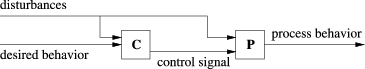
The feedforward control structure
- Feedback control:
-
In Fig. 2 the feedback control structure is shown [4]. In contrast to the feedforward control structure, here the behavior of the outputs is coupled back to the controller (hence the name feedback). This structure is also often referred to as “closed‐loop” control.
Figure 2 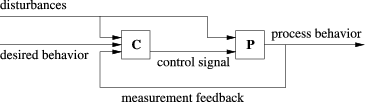
The feedback control structure
The main advantages of a feedback controller over a feedforward controller are that (1) it may have a quicker response (resulting in better performance), (2) it may correct undesired offsets in the output, (3) it may suppress unmeasurable disturbances that are observable through the output only, and (4) it may stabilize an unstable system.
- Optimal control:
-
Optimal control is a control methodology that formulates a control problem in terms of a performance function, also called an objective function [73]. This function expresses the performance of the system over a given period of time, and the goal of the controller is to find the control signals that result in optimal performance. Depending on the mathematical description of the control problem there exist several methods for the optimization of the control input including analytic and numerical approaches. Optimal control can be considered as a feedforward control approach.
- Model predictive control:
-
Model predictive control (MPC) is an extension of the optimal control framework [15,79]. In Fig. 3 the block diagram of MPC is shown.
Figure 3 
The model predictive control (MPC) structure
In MPC, at each time step k the optimal control signal is computed (by numerical optimization) over a prediction horizon of \( { N_{\mathrm{p}} } \) steps. A control horizon \( { N_{\mathrm{c}} (< N_{\mathrm{p}} } \)) can be selected to reduce the number of variables and to improve the stability of the system. Beyond the control horizon the control signal is usually taken to be constant. From the resulting optimal control signal only the first sample of the computed control signal is applied to the process. In the next time step \( { k+1 } \), a new optimization is performed with a prediction horizon that is shifted one time step ahead, and of the resulting control signal again only the first sample is applied, and so on. This scheme, called rolling horizon, allows for updating the state from measurements, or even for updating the model in every iteration step.
In other words, MPC is equivalent to optimal control extended with feedback. The advantage of updating the state through feedback is that this results in a controller that has a low sensitivity to prediction errors. Regularly updating the prediction model results in an adaptive control system, which could be useful in situations where the model significantly changes, such as in case of incidents or changing weather conditions.


Bibliography
Primary Literature
Alessandri A, Di Febbraro A, Ferrara A, Punta E (1999) Nonlinear optimization for freeway control using variable‐speed signaling. IEEE Trans Veh Technol 48(6):2042–2052
Algers S, Bernauer E, Boero M, Breheret L, Di Taranto C, Dougherty M, Fox K, Gabard J-F (2000) SMARTEST – Final report for publication. Technical report, ITS, University of Leeds. http://www.its.leeds.ac.uk/projects/smartest. Accessed on 22 July 2008
André M, Hammarström U (2000) Driving speeds in europe for pollutant emissions estimation. Transp Res Part D 5(5):321–335
Åström KJ, Wittenmark B (1997) Computer Controlled Systems, 3rd edn. Prentice Hall, Upper Saddle River
Banks JH (2005) Metering ramps to divert traffic around bottlenecks: Some elementary theory. Transp Res Rec 1925:12–19
Bell MGH (2000) A game theory approach to measuring the performance reliability of transport networks. Transp Res Part B 34(6):533–545
Bellemans T (2003) Traffic Control on Motorways. Ph.D. Thesis, Katholieke Universiteit Leuven, Leuven. ftp://ftp.esat.kuleuven.ac.be/pub/SISTA/bellemans/PhD/03-82.pdf. Accessed on 22 July 2008
Bellemans T, De Schutter B, De Moor B (2006) Model predictive control for ramp metering of motorway traffic: A case study. Control Eng Practice 14:757–767
Bellemans T, De Schutter B, Wets G, De Moor B (2006) Model predictive control for ramp metering combined with extended kalman filter‐based traffic state estimation. In: Proceedings of the 2006 IEEE Intelligent Transportation Systems Conference (ITSC 2006), Toronto, Canada, pp 406–411
Bishop R (2005) Intelligent vehicle technology and trends. In: Walker J (ed) Artech House ITS Library. Artech House, Boston
Braess D (1968) Über ein Paradoxon aus der Verkehrsplanung. Unternehmensforsch 12:258–268
Branston D (1976) Models of single lane time headway distributions. Transp Sci 10:125–148
Brownfield J, Graham A, Eveleigh H, Maunsell F, Ward H, Robertson S, Allsop R (2003) Congestion and accident risk. In: Technical report, Road Safety Research Report no. 44. Department for Transport, London
Byon Y-J, Shalaby A, Abdulhai B (2006) Travel time collection and traffic monitoring via GPS technologies. In: Proceedings of the 2006 IEEE Intelligent Transportation Systems Conference (ITSC 2006), Toronto, Canada, pp 677–682
Camacho EF, Bordons C (1995) Model Predictive Control in the Process Industry. Springer, Berlin
Cambridge Systematics, Inc. (2001) Twin Cities Ramp Meter Evaluation – Final Report. Cambridge Systematics, Inc., Oakland. Prepared for the Minnesota Department of Transportation
Carsten O, Tate F (2001) Intelligent speed adaptation: The best collision avoidance system? In: Proceedings of the 17th International Technological Conference on the Enhanced Safety of Vehicles, Amsterdam, Netherlands, pp 1–10
Carvell JD, Balke K Jr, Ullman J, Fitzpatrick K, Nowlin L, Brehmer C (1997) Freeway management handbook. Technical report. Federal Highway Administration, Department of Transport (FHWA, DOT), Washington DC, Report No. FHWA-SA-97-064
Castello P, Coelho C, Ninno ED (1999) Traffic monitoring in motorways by real-time number plate recognition. In: Proceedings of the 10th International Conference on Image Analysis and Processing, Venice, Italy, pp 1129–1131
Chaudhary NA, Messer CJ (2000) Ramp metering technology and practice. Technical Report 2121-1. Texas Transportation Institute, The Texas A&M University System, College Station
Chen A, Yang H, Lo HK, Tang WH (2002) Capacity reliability of a road network: An assessment methodology and numerical results. Transp Res Part B 36(3):225–252
Chen OJ, Hotz AF, Ben-Akiva ME (1997) Development and evaluation of a dynamic ramp metering control model. In: Proceedings of the 8th IFAC/IFIP/IFORS Symposium on Transportation Systems, Chania, Greece, June 1997, pp 1162–1168
Chien C-C, Zhang Y, Ioannou PA (1997) Traffic density control for automated highway systems. Automatica 33(7):1273–1285
Cools M, Moons E, Wets G (2007) Investigating the effect of holidays on daily traffic counts: A time series approach. Transp Res Record 2019:22–31
Cuena J, Hernández J, Molina M (1995) Knowledge‐based models for adaptive traffic management systems. Transp Res Part C 3(5):311–337
Daganzo CF (1994) The cell transmission model: A dynamic representation of highway traffic consistent with the hydrodynamic theory. Transp Res Part B 28B(4):269–287
Daganzo CF (1996) The nature of freeway gridlock and how to prevent it. In: Lesort JB (ed) Proceedings of the 13th International Symposium of Transportation and Traffic Theory, Lyon, France
Daganzo CF (1997) Fundamentals of Transportation and Traffic Operations. Pergamon, Kidlington
Di Febbraro A, Parisini T, Sacone S, Zoppoli R (2001) Neural approximations for feedback optimal control of freeway systems. IEEE Trans Veh Technol 50(1):302–312
Diakaki C, Papageorgiou M, McLean T (2000) Integrated traffic‐responsive urban corridor control strategy in Glasgow, Scotland. Transp Res Rec 1727:101–111
Elefteriadou L (1997) Freeway merging operations: A probabilistic approach. In: Proceedings of the 8th International Federation of Automatic Control (IFAC) Symposium on Transportation Systems, Chania, Greece, pp 1351–1356
Federal Highway Administration, US Department of Transportation (1995) Detection Technology for IVHS – Final Report Addendum. Technical report. Federal Highway Administration, US Department of Transportation, Washington, Contract DTFH61-91-C-00076, Report No. FHWA-RD-96-109
Federal Highway Administration, US Department of Transportation (1995) Detection Technology for IVHS – Task L Final Report. Technical report. Federal Highway Administration, US Department of Transportation, Washington, Contract DTFH61-91-C-00076, Report No. FHWA_RD-95-100
Fenton RE (1994) IVHS/AHS: Driving into the future. IEEE Control Syst Mag 14(6):13–20
Gartner NH, Improta G (eds) (1995) Urban Traffic Networks – Dynamic Flow Modeling and Control. Springer, Berlin
Gupta A, Maslanka VJ, Spring GS (1992) Development of prototype knowledge‐based expert system for managing congestion on massachusets turnpike. Transp Res Rec (1358):60–66
Hall FL, Agyemang-Duah K (1991) Freeway capacity drop and the definition of capacity. Transp Res Rec (1320):91–98
Hardman EJ (1996) Motorway speed control strategies using SISTM. In: Proceedings of the 8th International Conference on Road Traffic Monitoring and Control. IEE Conference Publication, no 422. London, 23–25 April 1996, pp 169–172
Hasan M, Jha M, Ben-Akiva M (2002) Evaluation of ramp control algorithms using microscopic traffic simulation. Transp Res Part C 10:229–256
Hedrick JK, Tomizuka M, Varaiya P (1994) Control issues in automated highway systems. IEEE Control Syst Mag 14(6):21–32
Hegyi A, De Schutter B, Hellendoorn J (2005) Model predictive control for optimal coordination of ramp metering and variable speed limits. Transp Res Part C 13(3):185–209
Hegyi A, De Schutter B, Hellendoorn J (2005) Optimal coordination of variable speed limits to suppress shock waves. IEEE Trans Intell Transp Syst 6(1):102–112
Hegyi A, Girimonte D, Babuška R, De Schutter B (2006) A comparison of filter configurations for freeway traffic state estimation. In: Proceedings of the International IEEE Conference on Intelligent Transportation Systems 2006, Toronto, Canada, 17–20 September 2006, pp 1029–1034
Helbing D (1997) Verkehrsdynamik – Neue physikalische Modellierungskonzepte. Springer, Berlin
Hellinga B, Van Aerde M (1995) Examining the potential of using ramp metering as a component of an ATMS. Transp Res Record 1494:75–83
Hernández J, Cuena J, Molina M (1999) Real-time traffic management through knowledge‐based models: The TRYS approach. In: ERUDIT tutorial on Intelligent Traffic Management Models. Helsinki, Finland, 3 August 1999. http://www.erudit.de/erudit/events/tc-c/tut990803.htm. Accessed on 23 July 2008
Hoogendoorn SP (1997) Optimal control of dynamic route information panels. In: Proceedings of the 4th World Congress on Intelligent Transportation Systems, IFAC Transportation Systems, Chania, Greece, pp 399–404
Hoogendoorn SP, Bovy PHL (2000) Continuum modelling of multiclass traffic flow. Transp Res Part B 34:123–146
Hoogendoorn SP, Bovy PHL (2001) State-of-the-art of vehicular traffic flow modelling. J Syst Control Eng – Proc Inst Mech Eng, Part I 215(14):283–303
Hotz A, Much C, Goblick T, Corbet E, Waxman A, Ashok K, Ben-Akiva M, Koutsopoulos H (1992) A distributed, hierarchical system architecture for advanced traffic management systems and advanced traffic information systems. In: Proceedings of the Second Annual Meeting of IVHS AMERICA, Newport Beach
http://www.auto21.ca/index.php. Accessed on 23 July 2008
http://www.cvisproject.org/. Accessed on 23 July 2008
http://www.damas.ift.ulaval.ca/projets/auto21/en/index.html. Accessed on 23 July 2008
http://www.path.berkeley.edu/. Accessed on 23 July 2008
Jacobson L, Henry K, Mehyar O (1989) Real-time metering algorithm for centralized control. Transp Res Record 1232:17–26
Jiang G, Gang L, Cai Z (2006) Impact of probe vehicles sample size on link travel time estimation. In: Proceedings of the 2006 IEEE Intelligent Transportation Systems Conference (ITSC 2006), Toronto, Canada, 2006, pp 891–896
Karimi A, Hegyi A, De Schutter B, Hellendoorn H, Middelham F (2004) Integration of dynamic route guidance and freeway ramp metering using model predictive control. In: Proceedings of the 2004 American Control Conference (ACC 2004), Boston, MA, USA, 30 June–2 July 2004, pp 5533–5538
Kell JH, Fullerton IJ, Mills MK (1990) Traffic Detector Handbook, Number FHWA-IP-90-002, 2nd edn. Federal Highway Administration, US Department of Transportation, Washington DC
Kerner BS (2002) Empirical features of congested patterns at highway bottlenecks. Transp Res Record (1802):145–154
Kerner BS (2004) The Physics of Traffic. Understanding Complex Systems. Springer, Berlin
Kerner BS (2007) Control of spatiotemporal congested traffic patterns at highway bottlenecks. IEEE Trans Intell Transp Syst 8(2):308–320
Kerner BS (2007) On-ramp metering based on three-phase traffic theory. Traffic Eng Control 48(1):28–35
Klein LA, Kelley MR, Mills MK (1997) Evaluation of overhead and in‐ground vehicle detector technologies for traffic flow measurement. J Test Evaluation (JTEVA) 25(2):215–224
Klein LA, Mills MK, Gibson DRP (2006) Traffic Detector Handbook, Number FHWA-HRT-06-108, 3rd edn. Federal Highway Administration, US Department of Transportation, Washington DC
Kotsialos A, Papageorgiou M (2005) A hierarchical ramp metering control scheme for freeway networks. In: Proceedings of the American Control Conference, Portland, OR, USA, 8–10 June 2005, pp 2257–2262
Kotsialos A, Papageorgiou M, Middelham F (2001) Optimal coordinated ramp metering with advanced motorway optimal control. In: Proceedings of the 80th Annual Meeting of the Transportation Research Board, vol 3125. Washington DC
Kotsialos A, Papageorgiou M, Mangeas M, Haj-Salem H (2002) Coordinated and integrated control of motorway networks via non‐linear optimal control. Transp Res C 10(1):65–84
Kraan M, van der Zijpp N, Tutert B, Vonk T, van Megen D (1999) Evaluating networkwide effects of variable message signs in the netherlands. Transp Res Record 1689:60–67
Kühne RD (1991) Freeway control using a dynamic traffic flow model and vehicle reidentification techniques. Transp Res Record 1320:251–259
Lee HY, Lee H-W, Kim D (1999) Empirical phase diagram of traffic flow on highways with on-ramps. In: Helbing D, Herrmann HJ, Schreckenberg M, Wolf DE (eds) Traffic and Granular Flow '99. Springer, Berlin
Lenz H, Sollacher R, Lang M (2001) Standing waves and the influence of speed limits. In: Proceedings of the European Control Conference 2001, Porto, Portugal, pp 1228–1232
Levinson D, Zhang L (2006) Ramp meters on trial: Evidence from the twin cities metering holiday. Transp Res Part A 40A:810–828
Lewis FL (1992) Applied Optimal Control and Estimation. Prentice Hall, Upper Saddle River
Li PY, Horowitz R, Alvarez L, Frankel J, Robertson AM (1995) Traffic flow stabilization. In: Proceedings of the American Control Conference, Seattle, Washington, June 1995, pp 144–149
Lighthill MJ, Whitham GB (1955) On kinematic waves, II. A theory of traffic flow on long crowded roads. Proc Royal Soc 229A(1178):317–345
Lin P-W, Chang G-L (2007) A generalized model and solution algorithm for estimation of the dynamic freeway origin‐destination matrix. Transp Res Part B, 41B:554–572
Little R, Rubin D (1987) Handbook of Transportation Science. Wiley, New York
Lo HK, Luo XW, Siu BWY (2006) Degradable transport network: Travel time budget of travelers with heterogeneous risk aversion. Transp Res Part B 40(9):792–806
Maciejowski JM (2002) Predictive Control with Constraints. Prentice Hall, Harlow
Maerivoet S, De Moor B (2005) Cellular automata models of road traffic. Phys Rep 419(1):1–64
May AD (1990) Traffic Flow Fundamentals. Prentice Hall, Englewood Cliffs
McDonald M, Hounsell NB, Njoze SR (1995) Strategies for route guidance systems taking account of driver response. In: Proceedings of 6th Vehicle Navigation and Information Systems Conference, Seattle, WA, July 1995, pp 328–333
Middelham F (1999) A synthetic study of the network effects of ramp metering. Technical report. Transport Research Centre (AVV), Dutch Ministry of Transport, Public Works and Water Management, Rotterdam
Middelham F (2003) State of practice in dynamic traffic management in The Netherlands. In: Proceedings of the 10th IFAC Symposium on Control in Transportation Systems (CTS 2003), Tokyo, Japan, August 2003
Middleton D, Gopalakrishna D, Raman M (2002) Advances in traffic data collection and management. Technical Report BAT-02-006. Texas Transportation Institute, Cambridge Systematics Inc., Washington. http://www.itsdocs.fhwa.dot.gov/JPODOCS/REPTS_TE/13766.html. Accessed on 23 July 2008
Molina M, Hernández J, Cuena J (1998) A structure of problem‐solving methods for real-time decision support in traffic control. Int J Human-Computer Stud 49:577–600
Papageorgiou M (1980) A new approach to time-of-day control based on a dynamic freeway traffic model. Transp Res Part B, 14B:349–360
Papageorgiou M (1983) A hierarchical control system for freeway traffic. Transp Res Part B, 17B(3):251–261
Papageorgiou M (1998) Some remarks on macroscopic traffic flow modelling. Transp Res Part A 32(5):323–329
Papageorgiou M (ed) (1991) Concise Encyclopedia of Traffic & Transportation Systems. Pergamon
Papageorgiou M, Kotsialos A (2000) Freeway ramp metering: An overview. In: Proceedings of the 3rd Annual IEEE Conference on Intelligent Transportation Systems (ITSC 2000), Dearborn, Michigan, USA, October 2000, pp 228–239
Papageorgiou M, Kotsialos A (2002) Freeway ramp metering: An overview. IEEE Trans Intell Transp Syst 3(4):271–280
Papageorgiou M, Messmer A (1991) Dynamic network traffic assignment and route guidance via feedback regulation. Transp Res Rec 1306:49–58
Papageorgiou M, Blosseville J-M, Hadj-Salem H (1990) Modelling and real-time control of traffic flow on the southern part of Boulevard Périphérique in Paris: Part I: Modelling. Transp Res Part A, 24A(5):345–359
Papageorgiou M, Blosseville J-M, Hadj-Salem H (1990) Modelling and real-time control of traffic flow on the southern part of Boulevard Périphérique in Paris: Part II: Coordinated on-ramp metering. Transp Res Part A, 24A(5):361–370
Papageorgiou M, Hadj-Salem H, Blosseville J-M (1991) ALINEA: A local feedback control law for on-ramp metering. Transp Res Rec (1320):58–64
Papageorgiou M, Hadj-Salem H, Middelham F (1997) ALINEA local ramp metering – summary of field results. Transp Res Rec 1603:90–98
Papageorgiou M, Wang Y, Kosmatopoulos E, Papamichail I (2007) ALINEA maximizes motorway throughput – An answer to flawed criticism. Traffic Eng Control 48(6):271–276
Payne HJ (1971) Models of freeway traffic and control. Simul Counc Proc 1:51–61
Rees I (1995) Orbital decongestant. Highways 63(5):17–18
Rees T, Harbord B, Dixon C, Abou-Rhame N (2004) Speed‐control and incident detection on the M25 controlled motorway (summary of results 1995–2002). Technical Report PPR033, TRL (UK's Transport Research Laboratory), Wokingham
Richards PI (1956) Shock waves on the highway. Oper Res 4:42–51
Ritchie SG (1990) A knowledge‐based decision support architecture for advanced traffic management. Transp Res Part A, 24A(1):27–37
Schik P (2003) Einfluss von Streckenbeeinflussungsanlagen auf die Kapazität von Autobahnabschnitten sowie die Stabilität des Verkehrsflusses. Ph.D. Thesis, Universität Stuttgart
Shladover SE, Desoer CA, Hedrick JK, Tomizuka M, Walrand J, Zhang WB, McMahon DH, Peng H, Sheikholesham S, McKeown N (1991) Automatic vehicle control developments in the PATH program. IEEE Trans Veh Technol 40(1):114–130
Sisiopiku VP (2001) Variable speed control: Technologies and practice. In: Proceedings of the 11th Annual Meeting of ITS America, Miami, pp 1–11
Slotine JE, Li W (1991) Applied Nonlinear Control. Prentice Hall, New Jersey
Smith BL, Zhang H, Fontaine MD, Green MW (2004) Wireless location technology based traffic monitoring: Critical assessment and evaluation of an early‐generation system. J Transp Eng 130(5):576–584
Smulders S (1990) Control of freeway traffic flow by variable speed signs. Transp Res Part B, 24B(2):111–132
Smulders SA, Helleman DE (1998) Variable speed control: State-of-the-art and synthesis. In: Road Transport Information and Control, number 454 in Conference Publication, IEE, 21–23 April 1998, pp 155–159
Soriguera F, Thorson L, Robuste F (2007) Travel time measurement using toll infrastructure. In: Proceedings of the 86th Annual Meeting of the Transportation Research Board, CDROM paper 07-1389.pdf
Taylor CJ, Young PC, Chotai A, Whittaker J (1998) Nonminimal state space approach to multivariable ramp metering control of motorway bottlenecks. IEE Proc – Control Theory Appl 146(6):568–574
Taylor MAP (1999) Dense network traffic models, travel time reliability and traffic management. I: General introduction. J Adv Transp 33(2):218–233
Taylor MAP (1999) Dense network traffic models, travel time reliability and traffic management. II: Application to network reliability. J Adv Transp 33(2):235–251
Taylor MAP, Woolley JE, Zito R (2000) Integration of the global positioning system and geographical information systems for traffic congestion studies. Transp Res Part C, 8C:257–285
Transportation Research Board (1998) Managing speed: Review of current practice for setting and enforcing speed limits. In: TRB Special Report 254, Transportation Research Board, Committee for Guidance on Setting and Enforcing Speed Limits. National Academy Press, Washington
Treiber M, Hennecke A, Helbing D (2000) Congested traffic states in empirical observations and microscopic simulation. Phys Rev E 62:1805–1824
Tsugawa S, Kato S, Tokuda K, Matsui T, Fujii H (2000) An architecture for cooperative driving of automated vehicles. In: Proceedings of the IEEE Intelligent Transportation Symposium, Dearborn, MI, USA 2000, pp 422–427
Vahidi A, Eskandarian A (2003) Research advances in intelligent collision avoidance and adaptive cruise control. IEEE Trans Intell Transp Syst 4(3):143–153
van Arem B, van Driel CJG, Visser R (2006) The impacts of cooperative adaptive cruise control on traffic‐flow characteristics. IEEE Trans Intell Transp Syst (4):429–436
van den Berg M, Bellemans T, De Schutter B, De Moor B, Hellendoorn J (2005) Control of traffic with anticipative ramp metering. In: Proceedings of the 84th Annual Meeting of the Transportation Research Board, Washington DC, 2005 CDROM paper 05-0252, pp 166–174
van den Hoogen E, Smulders S (1994) Control by variable speed signs: Results of the Dutch experiment. In: Proceedings of the 7th International Conference on Road Traffic Monitoring and Control, IEE Conference Publication No. 391, London, England, 26–28 April 1994, pp 145–149
Varaiya P (1993) Smart cars on smart roads: Problems of control. IEEE Trans Autom Control 38(2):195–207
Wang Y, Papageorgiou M (2005) Real-time freeway traffic state estimation based on extended Kalman filter: A general approach. Transp Res Part B 39(2):141–167
Wang Y, Papageorgiou M, Messmer A (2003) A predictive feedback routing control strategy for freeway network traffic. In: Proceedings of the 82nd Annual Meeting of the Transportation Research Board, Washington DC, January 2003
Wang Y, Papageorgiou M, Messmer A (2006) RENAISSANCE A unified macroscopic model-based approach to real-time freeway network traffic surveillance. Transp Res Part C, 14C:190–212
Wattleworth JA (1965) Peak‐period analysis and control of a freeway system. Highw Res Rec 157:1–21
Wilkie JK (1997) Using variable speed limit signs to mitigate speed differentials upstream of reduced flow locations. Technical report. Department of Civil Engineering, Texas A& M University, College Station, Prepared for CVEN 677 Advanced Surface Transportation Systems, Report No. SWUTC/97/72840-00003-2
Williams B (1996) Highway control. IEE Rev 42(5):191–194
Wolf DE (1999) Cellular automata for traffic simulations. Physica A 263:438–451
Zhang H, Ritchie SG (1994) Real-time decision‐support system for freeway management and control. J Comput Civ Eng 8(1):35–51
Zhang L (2007) Traffic diversion effect of ramp metering at the individual and system levels. In: Proceedings of the 86th Annual Meeting of the Transportation Research Board, Washington DC, January 2007, CDROM paper 07-2087
Books and Reviews
We refer the interested reader to the following references
in the various fields that have been discussed in thischapter:
Control: General introduction [4], optimal control [73], model predictive control [15,79], nonlinear control [107],
Traffic flow modeling: General overviews [48,49], cell transmission model [26], Kerner's three-phase theory [60], microscopic simulation models [2], cellular automata [80],
Ramp metering: Overviews of ramp metering strategies [18,91], field test and simulation studies [39],
Speed limit systems: Overviews of practical speed limit systems [106,128],
Intelligent vehicles: Overview [10],
Sensor technologies: Overviews [32,33,63,64]
Author information
Authors and Affiliations
Editor information
Editors and Affiliations
Rights and permissions
Copyright information
© 2009 Springer-Verlag
About this entry
Cite this entry
Hegyi, A., Bellemans, T., De Schutter, B. (2009). Freeway Traffic Management and Control. In: Meyers, R. (eds) Encyclopedia of Complexity and Systems Science. Springer, New York, NY. https://doi.org/10.1007/978-0-387-30440-3_232
Download citation
DOI: https://doi.org/10.1007/978-0-387-30440-3_232
Publisher Name: Springer, New York, NY
Print ISBN: 978-0-387-75888-6
Online ISBN: 978-0-387-30440-3
eBook Packages: Physics and AstronomyReference Module Physical and Materials ScienceReference Module Chemistry, Materials and Physics