Network Design in Enterprises’ Green Growth Model

Abstract

Network design refers to the process of locating and arranging the capacities of suppliers, manufacturing plants, distribution centers, retailers, warehouses, and other related facilities involved in the value-added activities of a value chain. Network design acts as decision-making content for enterprises to implement the green growth model. It belongs to the strategic level of value chain reconstruction and directly determines the economic and environmental performance of enterprises. Given the new requirements of the enterprises’ green growth model for network design, efficient and reasonable network design decision-making is a key factor to help enterprises realize a green transformation. This chapter starts by introducing the basic framework and methods of network design. Then, focusing on network design considering carbon emissions, an optimization model and solution algorithm are developed, and the influence of carbon emissions on the network design is analyzed. Finally, shifting the focus to the network design of waste product collection channels, a closed-loop supply chain network model of manufacturer-remanufacturing and retailer-recycling is developed. This is used to analyze the influencing factors and mechanisms of network efficiency under different waste product collection channels and reuse technologies.

5.1 Basic Framework and Methods of Network Design

5.1.1 Relationship Between Network Design and Enterprises’ Green Growth Model

• (1) Network Design

The value chain network is a complex network composed of multiple entities and the relationships between them [1], as shown in Fig. 5.1. The design and optimization of the value chain network is one of the key decision-making contents for enterprises to implement the green growth model, which belongs to the strategic level [2]. The value chain network includes entities such as suppliers, manufacturers, retailers, and customers, involves value-added activities such as raw material supply, production, finished product storage, transportation, and after-sales service, and considers material, cash, and information flows between entities. Network design and optimization affects the strategic layout, basic investment, production and operation planning, environmental protection, and other aspects, and directly determines the enterprise’s economic and environmental performance. A network design scheme is bound to be very difficult to implement or costly to change after capital has been invested and the facilities completed. That is why carrying out an efficient and reasonable network design is an important decision-making problem.

Fig. 5.1

Schematic diagram of value chain network

Network design and optimization usually includes the following decision-making aspects:

• Determining roles of the various facilities involved in value-added activities.

• Determining the appropriate number of facilities.

• Determining the location of each facility.

• Determining the services provided by each facility.

• Determining distribution, transportation, inventory, and so on.

The common goal of network design is to find a balance between maintaining a certain service level and minimizing the total of all costs including production, purchase, inventory, facilities, and transportation.

• (2) Requirements of Enterprises’ Green Growth Model for Network Design

As a result of increasingly prominent environmental problems, there is an inevitable tendency of enterprises implementing the green growth model. Unlike traditional network design, enterprises’ green growth model simultaneously brings economic and social benefits into the decision-making category. In addition, the decision-making objectives are more complex and the content more diverse. Network design of the value chain based on the enterprises’ green growth model has two key perspectives.

First, it takes account of social and environmental benefits in addition to the traditional value chain network design. The traditional value chain network design primarily considers the minimization of operational costs under the condition of meeting a certain service level. However, the enterprises’ green growth model requires that network design decision-making pays attention to not only economic factors, but also the impact on the environment and society. Thus, value chain network design from this perspective considers optimization objectives other than that of cost-minimization. For example, in the case of the green network design for multi-cycle, multi-type products, and limited capacity, Rad et al. developed an optimization model that minimized carbon emissions and total cost simultaneously, with management insights being provided through numerical analysis [3].

Second, it is necessary to design and optimize the value chain network in combination with new forms of industry or business models. For example, network design and optimization of a closed-loop supply chain is promoted by an increase in resource pressure, shortening of the product life cycle, and improvement of consumers’ awareness of environmental protection. Contrary to traditional network design and optimization, activities such as recycling and remanufacturing of waste products and accompanying activities, including collection, storage, and transportation, must be considered. Thus, value chain network design from this perspective mainly considers new network design and optimization problems and mathematical models. For example, Prakash et al. developed an optimization model based on mixed-integer programming for a closed-loop supply chain network design problem with the consideration of supply, transportation, and demand uncertainties, and provided a case analysis based on an e-commerce company in India [4].

5.1.2 Basic Framework of Network Design

Based on the process of network design and optimization, the value chain network should first be transformed into an abstract network. The entities in the value chain network, or facilities involved in value-added activities should be abstracted as vertices, while the relationships between entities, namely material, cash, or information flows, should be abstracted as directed arcs. This forms an abstract value chain network $G(V,A)$, where the set of vertices $V$ represents the entities or facilities in the value chain network, and the set of arcs $A$ represents the flows. The general objective of network design is to minimize the total cost. Some basic frameworks of network design are introduced below.

• (1) Transport Model

The transport model is a classic network design and optimization decision model, as shown in Fig. 5.2. Let the network have $n$ suppliers and $m$ customers. The maximum supply of each supplier is $K_i$, while the demand of each customer is $D_j$. Additionally, the unit transportation cost from each supplier to each customer is $c_{ij}$. It is necessary to determine which customers each supplier provides materials to while ensuring that the amount of materials obtained by each customer can meet their demands. The objective is, thus, to minimize the total transportation cost. The decision variable $x_{ij}$ represents the quantity of materials provided by each supplier to each customer. The mathematical model is developed as follows.

Fig. 5.2

Schematic diagram of transport model

$$ \min \sum\limits_{i = 1}^n {\sum_{j = 1}^m {c_{ij} x_{ij} } } $$

(5.1)

s.t.

$$ \begin{array}{*{20}c} {\sum\limits_{i = 1}^n {x_{ij} } = D_j } & {j \in \{ 1,2, \ldots ,m\} } \\ \end{array} $$

(5.2)

$$ \begin{array}{*{20}c} {\sum\limits_{j = 1}^m {x_{ij} } \le K_i } & {i \in \{ 1,2, \ldots ,n\} } \\ \end{array} $$

(5.3)

$$ \begin{array}{*{20}c} {x_{ij} \ge 0} & {i \in \{ 1,2, \ldots ,n\} ;j \in \{ 1,2, \ldots ,m\} } \\ \end{array} $$

(5.4)

The objective function (5.1) minimizes the total transportation cost given the following constraints. Constraint (5.2) ensures that the demands of each customer are satisfied. Constraint (5.3) means that the quantity of materials provided by each supplier does not exceed the maximum supply. Constraint (5.4) outlines the range of values of the decision variables.

• (2) Facility Location Model

The facility location model considers the selection of alternative suppliers based on the transport model, as shown in Fig. 5.3. Again, $n$ alternative suppliers and $m$ customers are considered. The maximum supply and fixed cost of each alternative supplier are $K_i$ and $f_i$, respectively, while the demand of each customer is $D_j$. Additionally, the unit transportation cost from each alternative supplier to each customer is $c_{ij}$. It is necessary to determine which alternative suppliers are selected and which customers each supplier then provides materials to, while ensuring that the amount of materials obtained by each customer can meet their demands. Thus, the objective is to minimize the total fixed and transportation costs. As before, the decision variable $x_{ij}$ represents the quantity of materials provided by each supplier for each customer. The binary decision variable $y_i$, equaling 1 or 0, represents if the alternative supplier is selected or not. The mathematical model is developed as follows.

Fig. 5.3

Schematic diagram of facility location model

$$ \min \left( {\sum\limits_{i = 1}^n {f_i y_i } + \sum\limits_{i = 1}^n {\sum\limits_{j = 1}^m {c_{ij} x_{ij} } } } \right) $$

(5.5)

s.t.

Constraint (5.2)

$$ \begin{array}{*{20}c} {\sum\limits_{j = 1}^m {x_{ij} } \le K_i y_i } & {i \in \{ 1,2, \ldots ,n\} } \\ \end{array} $$

(5.6)

$$ \begin{array}{*{20}c} {x_{ij} \ge 0;y_i \in \{ 0,1\} } & {i \in \{ 1,2, \ldots ,n\} ;j \in \{ 1,2, \ldots ,m\} } \\ \end{array} $$

(5.7)

The objective function (5.5) minimizes the total fixed and transportation costs subject to the following constraints. Constraint (5.6) ensures that only the selected alternative suppliers can provide materials, and the amount of materials provided by each one does not exceed its maximum supply. Constraint (5.7) outlines the range of values of the decision variables.

• (3) Multi-Level Facility Location Model

The multi-level facility location model is an extension of the facility location model, as it further considers the multi-level network. It is closer to reality and the most commonly used basic model in current research. The following description illustrates a relatively simple multi-level value chain network, as shown in Fig. 5.4.

Fig. 5.4

Schematic diagram of multi-level facility location model

The network comprises $l$ raw material suppliers, $n$ manufacturing plants, $t$ warehouses, and $m$ customers. The supplies of each raw material supplier, outputs of each manufacturing plant, storage capacities of each warehouse, and demands of each customer are $S_h$, $K_i$, $W_e$, and $D_j$, respectively. The fixed construction costs of the manufacturing plants and warehouses are $f_i$ and $f_e$, respectively. The unit transportation costs from each supplier to each manufacturing plant, each manufacturing plant to each warehouse, and each warehouse to each customer are denoted by $c_{hi}$, $c_{ie}$, and $c_{ej}$, respectively. It is required to determine the location scheme of manufacturing plants and warehouses, as well as the entire transportation scheme, so that the amount of materials obtained by each customer can meet their demands. Thus, the objective is to minimize the total fixed and transportation costs. The decision variables $x_{hi}$, $x_{ie}$, and $x_{ej}$ represent the transportation volumes at each level of the value chain network, while the binary decision variables $y_i$ and $y_e$ represent if the respective manufacturing plants and warehouses are selected or not. The mathematical model is developed as follows.

$$ \min \left( {\sum_{i = 1}^n {f_i y_i } + \sum_{e = 1}^t {f_e y_e } + \sum_{h = 1}^l {\sum_{i = 1}^n {c_{hi} x_{hi} } + } \sum_{i = 1}^n {\sum_{e = 1}^t {c_{ie} x_{ie} } + } \sum_{e = 1}^t {\sum_{j = 1}^m {c_{ej} x_{ej} } } } \right) $$

(5.8)

s.t.

$$ \begin{array}{*{20}c} {\sum\limits_{i = 1}^n {x_{hi} } = S_h } & {h \in \{ 1,2, \ldots ,l\} } \\ \end{array} $$

(5.9)

$$ \begin{array}{*{20}c} {\sum\limits_{h = 1}^l {x_{hi} } - \sum\limits_{e = 1}^t {x_{ie} } \ge 0} & {i \in \{ 1,2, \ldots ,n\} } \\ \end{array} $$

(5.10)

$$ \begin{array}{*{20}c} {\sum\limits_{e = 1}^t {x_{ie} } \le K_i y_i } & {i \in \{ 1,2, \ldots ,n\} } \\ \end{array} $$

(5.11)

$$ \begin{array}{*{20}c} {\sum\limits_{i = 1}^n {x_{ie} } - \sum\limits_{j = 1}^m {x_{ej} } \ge 0} & {e \in \{ 1,2, \ldots ,t\} } \\ \end{array} $$

(5.12)

$$ \begin{array}{*{20}c} {\sum\limits_{j = 1}^m {x_{ej} } \le W_e y_e } & {e \in \{ 1,2, \ldots ,t\} } \\ \end{array} $$

(5.13)

$$ \begin{array}{*{20}c} {\sum\limits_{e = 1}^t {x_{ej} } = D_j } & {j \in \{ 1,2, \ldots ,m\} } \\ \end{array} $$

(5.14)

$$ \begin{gathered} x_{hi} ,x_{ie} ,x_{ej} \ge 0;y_i ,y_e \in \{ 0,1\} \hfill \\ \, h \in \{ 1,2, \ldots ,l\} ;i \in \{ 1,2, \ldots ,n\} ;e \in \{ 1,2, \ldots ,t\} ;j \in \{ 1,2, \ldots ,m\} \hfill \\ \end{gathered} $$

(5.15)

The objective function (5.8) minimizes the total fixed and transportation costs subject to the following constraints. Constraint (5.9) indicates the supply constraint of the suppliers. Constraints (5.10) and (5.11) indicate the output constraints of the manufacturing plants. Constraints (5.12) and (5.13) indicate the storage constraints of the warehouses. Constraint (5.14) ensures that the demands of each customer are met, and constraint (5.15) outlines the range of values of the decision variables.

The three optimization models of network design described above constitute the basic framework for network design with each model having its own scope of application. The transport model is applicable to situations where the fixed cost does not need to be considered, whereas the facility location model is applicable to situations where the fixed and transportation costs need to be considered simultaneously. The multi-level facility location model considers a value chain network with a multi-level structure. With the deepening of research and closer correlation with real situations, the multi-level facility location model has become the most commonly used basic network design model in research as it matches the actual value chain network structure and incorporates a variety of considerations. However, these network design models do not consider the requirements of enterprises’ green growth model. According to the analysis in Sect. 5.1.1, the value chain network design based on the enterprises’ green growth model adds the decision-making content of environmental performance to the above models, such as the objective of reducing carbon emissions. New network design models, including recycling, remanufacturing, and other activities can also be considered, such as the network design for a closed-loop supply chain. Sections 5.2 and 5.3 of this chapter will introduce relevant research and analyze them in detail.

5.1.3 Solution Methods of Network Design

While a value chain network is a relatively complex network, network design, as a decision-making problem, is also complex. Depending on the characteristics of specific problems and the difficulty and accuracy requirements of the solutions, network design problems can usually be solved using three types of methods: exact algorithm, heuristic algorithm, and system simulation.

• (1) Exact Algorithm

Exact algorithm is an algorithm that finds the optimal solution of a problem using a linear approach. The optimal solution can be determined through enumeration and iteration. The network design scheme generated by an exact algorithm must be the optimal scheme. However, due to the non-deterministic polynomial time complexity of NP-hard problems. Although an exact algorithm can obtain the optimal solution of a problem in theory, the computation time required is astronomical. Therefore, exact algorithms are only effective when dealing with small-scale NP-hard problems. Once the scale of an NP-hard problem is relatively large, the exact algorithm is often powerless because it cannot solve the problem in a reasonable time. Typical exact algorithms include the tabular method, branch-and-bound approach, cutting-plane approach, dynamic programming, etc. Usually, once the mathematical model is developed, the optimal solution can be generated using relevant software such as Lingo and CPLEX.

Given these characteristics of exact algorithms, the network design problems most suitable to be solved by them should be P-problems or small-scale NP-hard problems. The transport model is a type of network design the exact algorithm is well suited to solve because it is a linear programming model that can be solved in polynomial time. The most commonly used method is the tabular method, which obtains the optimal solution based on a supply and demand balance table. However, for the facility location and multi-level facility location models, the exact algorithm can only solve small-scale problems.

• (2) Heuristic Algorithm

The exact algorithm requires infinite time to find the optimal solution for a large-scale NP-hard problem. The heuristic algorithm can solve this defect and find a better solution in a limited time; however, this solution may not be optimal. The key advantage of the heuristic algorithm is that it aims to obtain a solution with acceptable quality in a reasonable time range to provide a satisfactory scheme for the decision maker. Therefore, it is suitable for solving large-scale NP-hard problems and dealing with the practical applications of network design. The basic ideas of many heuristic algorithms originate from biological, physical, social, and natural phenomena. Commonly used heuristic algorithms include genetic, simulated annealing, ant colony algorithms, etc.

Due to the above advantages, heuristic algorithms have become the most commonly used solution method in network design and optimization. For example, Farshbaf-Geranmayeh et al. studied a closed-loop supply chain network design problem, proposed a quantity estimation function based on return product prices, and developed a network design model considering the pricing of return products, material flow, inventory, and manufacturing/remanufacturing decisions. This was then, solved using a simulated annealing algorithm [5].

• (3) System Simulation

Both exact and heuristic algorithms are aimed at static systems that do not consider changes in parameters with time. By contrast, tools based on simulation models can analyze dynamic or extremely complex systems. System simulations are methods based on system theory, control theory, mathematical statistics, information technology, and computer technology. Using computers, or other special physical equipment as tools, system simulation is used to experiment with real or hypothetical systems. The experimental results are analyzed and studied with the help of expert experience, statistical data, and system data. The system simulation method can simulate the operation and then apply the results of the experiments to real systems. Common system simulation methods include the Monte Carlo and system dynamics simulations.

Scholars often use system simulations to study network design problems. For example, Ozkan et al. conducted an in-depth analysis of the reliabilities of logistics networks through a Monte Carlo simulation. They comprehensively generated several cases of different sizes for a variety of scenarios, tested them, and drew conclusions [6]. However, system simulations can only deal with network design under preset scenarios. If we consider changing the structure, e.g., several customers want to change other warehouses to provide services, we will need to run the simulation model again. A detailed simulation model may require a very long time to execute the system to a certain level of accuracy, which means that the simulations usually provide very few schemes.

The applicable scenarios, strengths, and weaknesses of exact algorithm, heuristic algorithm, and system simulation are summarized in Table 5.1.

Table 5.1 Comparison of solution methods of network design

5.2 Network Design Considering Carbon Emissions

5.2.1 Impact of Carbon Emissions on the Value Chain of Enterprises

Governments and consumers regard carbon emissions as one of the most important environmental impact indicators [7]. With the growing global focus on carbon reduction, governments and consumers are forcing enterprises to reduce their carbon emissions. Many countries have formulated policies, laws, and regulations to restrict carbon emissions [8]. For example, China has established a leading group headed by the Premier of the State Council to address climate change, energy conservation, and emission reduction. The group is responsible for coordinating and formulating policies related to climate change [9]. An increasing number of enterprises are beginning to monitor carbon emissions during their business activities [10]. If manufacturers want to live up to their social responsibilities and maintain a competitive position, it is imperative to focus on carbon emissions [11]. Procter & Gamble has committed to reducing greenhouse gas emissions by 50% from its value chain by 2030. That amounts to a reduction of approximately 30 million metric tons of carbon emissions by the enterprise.¹

While reducing carbon emissions is necessary to improve the way enterprises consume energy, this results in increased costs in the short term. However, in the long run, reducing carbon emissions is the essence of the industrial structural transformation of enterprises; it is the process of enterprises moving from low-value and high-consumption industries to high-value and low-consumption industries. Therefore, reducing carbon emissions plays an important role in promoting the green growth of enterprises in the long run [12], and hence, constitutes an important goal of the green growth model of enterprises. As carbon emission reduction is a long-term process, achieving this reduction also involves designing a carbon emission reduction value chain for enterprises that can stimulate efficient emission reduction without hindering corporate benefits. This has become a key issue that enterprises are generally concerned about today.

5.2.2 Model of Network Design Considering Carbon Emissions

Product recycling is an effective method of reducing carbon emissions. The reverse logistics network structure of recycling activities affects the related transportation activities, which is the main source of CO₂ emissions [13]. Through the layout of facilities in a reverse logistics network, reducing the driving distance of vehicles plays an important role in reducing transportation related carbon emissions [14]. Therefore, it is important for enterprises to design their reverse logistics networks scientifically and thus reduce carbon emissions. When designing reverse logistics networks, enterprises must consider the carbon emissions generated by transportation. This will promote the reduction of carbon emissions while achieving sustainable development.

The Emissions Trading Scheme (ETS) is currently one of the most effective market mechanisms for reducing carbon emissions [15]. ETS has been widely adopted by the United Nations, the European Union, and many other governments. It is based on the “cap and trade” principle, that is, the government imposes a cap on CO₂ emissions, while each enterprise has a CO₂ emission credit. Enterprises must purchase the same number of carbon credits to meet their social obligations. The main goal of recycling is to maximize profits; therefore, it is typical for the cheapest recycling technology to be used in the recycling process. The ETS forces recycling enterprises to change the way their reverse supply chains operate. They must re-optimize their internal and external processes, design logistics networks, use emission-reducing transport modes to reduce CO₂ emissions, and invest in new carbon-reduction technologies. Can ETS contribute to reducing CO₂ emissions? How does ETS affect an enterprise’s reverse logistics network design? These issues will be discussed in this section.

In summary, this section considers an enterprise that adopts the ETS mechanism; its reverse logistics network is shown in Fig. 5.5. An enterprise’s reverse logistics network consists of centralized return centers (CRCs), remanufacturing facilities (RFs), initial collection points (ICPs), secondary markets, customer areas, and third-party recyclers. Customers’ recycled products are usually returned to the nearest ICP. Returned products are stored at the ICP and then sent to the CRC. The recycled products are inspected at the ICP to collect the used products that can be remanufactured. After being consolidated and sorted at the CRC, the returned products are shipped to RFs for remanufacturing. Finally, products that cannot be remanufactured or are defective during dismantling are sold to third-party recyclers. Remanufactured products are 50–70% cheaper than new products in the secondary market. These damaged products can be consumed through direct reuse or used as a substitute for raw materials within the industry. Therefore, there is no product disposal. The models constructed in this section are designed to minimize total CO₂ emissions and maximize the profits of reverse logistics networks. This reverse logistics network determines the collection period for the ICPs, optimal quantities and locations of the CRCs and ICPs, and distribution of recycling customers for the reverse logistics facility. To reduce CO₂ emissions and transportation costs during transportation, single distribution between reverse logistics facilities is allowed.

Fig. 5.5

Enterprises’ reverse logistics network adopted ETS mechanism

• (1) Assumptions of Remanufacturing Reverse Logistics Networks Considering Carbon Emission

  Before building the model, we state the following assumptions:

• • Due to the limited number of returned products that can be received from a single customer and the distance from the RF, the RF does not accept returned products sent directly by customers. Customers can only send the repaired product to the nearest ICPs, who will then send it to the CRC.

• • The ICP will send the received reworked products to the CRC on the same day, so that the ICP has sufficient capacity to accommodate the returned reworked products in the customer area.

• • The cost of transportation between the customer and ICP is borne by the customer.

• • During a given period, the daily number of products returned by the customer remains unchanged.

• • The returned product has a negligible waiting time for shipping between the ICP and the CRC.

• (2) Constituent Sets of the Remanufacturing Reverse Logistics Networks

I = {1,…, i}: customer point set

K = {1,…,k}: set of potential locations for CRCs

J = {1,…, j}: set of potential locations for ICPs

R = {1,…,r}: set of potential locations for RFs

• (3) Parameters of the Remanufacturing Reverse Logistics Network

w: Number of working days per year

r_i: The number of products returned per day in the customer area i, $\forall i \in I$.

f_j: Annual rental cost per ICP

v_k: The variable cost of building a CRC

f_k: Fixed cost of establishing a CRC

c: Collection costs for returned products

f_r^h: Fixed cost of remanufacturing product using technology h in RFs

b: Inventory cost per unit of product in ICP

v_r: Variable cost of manufacturing one more unit of product in RFs

d_jk: Distance from ICP j to CRC k

d_ij: Distance from customer i to ICP j

d_rs: RF r distance to secondary market

d_kr: Distance from CRC k to RF r

D: Maximum service range from ICP to designated customer area

V: Unit capacity level per CRC

L: Maximum capacity level per CRC

N: Government-regulated CO₂-equivalent caps

Β: Average recoverable percentage of returned products

Q: The capacity of per ICP

T: Maximum returned period for ICPs

M: An arbitrarily large number

s: The price at which remanufactured products are sold on the secondary market

p: Market price for buying and selling CO₂ credits

a: Income from the sale of one unit of defective product to a third-party recycling facility

COs^m: CO₂ emission factor per unit distance using transport mode m

CO^m: CO₂ emission factor per unit distance using transport mode m (no load)

CH^h: CO₂ emissions per unit of product using remanufacturing technology h in RFs

• (4) Mathematical Model

Total profits are used to evaluate the economic goals while total CO₂ emissions are used to evaluate environmental goals. The total CO₂ emissions and revenue-cost components of the objective functions can be calculated as follows:

• a. Income. Income consists of two parts. The first is the profit from the sale of remanufactured products on the secondary market. The second part is the profit made from selling defective products to the third-party recycling enterprises. Total revenue can then be expressed as $RE = s\sum_i {r_i } w\beta + a\sum_i {r_i } w\left( {1 - \beta } \right)$.

• b. Recovery costs. Recovery costs are the costs of collecting returned products from customers; it is equal to $CC = c\sum_i {r_i } w$.

• c. Fixed cost of acquiring technology. Different returned products may require different repair techniques. Thus, the fixed cost of technology acquisition is $HC = \sum_h {f_r^h Er^{_h } }$.

• d. Inventory costs. Inventory cost is the product storage cost of the ICP. That is $IC = bw\sum_i {r_i } X_{ij} \left( {\frac{T_j + 1}{2}} \right)$.

• e. Rental cost. The rental cost of ICP is $RCI = \sum_j {f_j Z_j }$.

• f. Remanufacturing costs. The remanufacturing cost of the RFs is $RC = v_r \beta \sum_i {r_i } w$.

• g. Establishing cost. The total fixed and variable costs of establishing a CRC are $ECK = \sum_k {G_k^l \left( {f_k + l \cdot v_k } \right)}$.

• h. Transportation cost. Transportation costs consist of three parts. The first part is the transportation cost from ICP j to CRC k. The second part is the transportation cost from the RF r to the secondary market. The third part is the transportation cost from CRC k to RF r. Thus, the total transportation cost is.

  $$ \begin{aligned} TC & = \sum_m {\sum_k {\sum_j {Et^m U_{jk} } \frac{w}{T_j }f\left( {U_{jk} ,d_{jk} } \right)} } + \sum_m {\sum_r {\sum_k {Et^m O_{kr} } wf\left( {O_{kr} ,d_{kr} } \right)} } \\ & \quad + \sum_m {\sum_r {Et^m wf\left( {\sum_k {O_{kr} \beta } ,d_{rs} } \right)} } \beta \sum_k {O_{kr} } . \\ \end{aligned} $$
  $$ \alpha = \left\{ {\begin{array}{*{20}l} 1 \hfill \\ {\alpha _1 } \hfill \\ {\alpha _2 } \hfill \\ {\alpha _3 } \hfill \\ {\alpha _4 } \hfill \\ \end{array} } \right.\quad \begin{array}{*{20}l} {U_{jk} \le p_1 } \hfill \\ {p_1 < U_{jk} \le p_2 } \hfill \\ {p_2 < U_{jk} \le p_3 } \hfill \\ {p_3< U_{jk} \le p_4 } \hfill \\ {U_{jk} > p_4 } \hfill \\ \end{array} \quad \gamma = \left\{ \begin{gathered} 1 \hfill \\ \gamma _1 \hfill \\ \gamma _2 \hfill \\ \gamma _3 \hfill \\ \gamma _4 \hfill \\ \end{gathered} \right.\quad \begin{array}{*{20}l} {d_{jk} \le q_1 } \hfill \\ {q_1 < d_{jk} \le q_2 } \hfill \\ {q_2 < d_{jk} \le q_3 } \hfill \\ {q_3< d_{jk} \le q_4 } \hfill \\ {d_{jk} > q_4 } \hfill \\ \end{array} $$

• i. CO₂ emission cost. The cost of buying or selling CO₂ credits: purchased cost >0, sold cost < 0. The ETS can sell credits if an enterprise’s emissions fall below the government-mandated cap. Otherwise, if the enterprise exceeds the cap, it needs to purchase the same amount of carbon credit. The emission costs are given as $EC = CO_{in} p$.

Both transportation and remanufacturing lead to high CO₂ emissions. The total CO₂ emissions consist of two components. The first part of comprises emissions comes from remanufacturing. The second part is the emissions from transport from ICP j to CRC k, RF r to the secondary market, and CRC k to RF r. Total emissions were calculated as follows:

$$ \begin{aligned} CO_{out} & = \sum_k {\left( {\sum_j {\left( {U_{jk} COs^m + CO^m } \right)d_{jk} \frac{w}{{T_j }}} } \right)} + \sum_h {Er^h \beta \sum_i {r_i } } w \\ & \quad + \sum_r {\left( {\sum_k {U_{kr} COs^m + CO^m } } \right)} d_{kr} w \\ & \quad + \sum_r {\left( {\sum_k {\beta U_{kr} COs^m + CO^m } } \right)} d_{rs} w \\ \end{aligned} $$

In summary, the network considering carbon emissions is as follows.

$$ Maximize\,OBJ_1 = E - \left( {CC + IC + HC + RC + RCI + ECK + EC + TC} \right) $$

(5.16)

$$ {\text{Minimize}}\,OBJ_2 = CO_{out} $$

(5.17)

Subject to

$$ \sum_k {W_{jk} } = Z_j ,\forall j \in J $$

(5.18)

$$ \sum_j {X_{ij} = 1,\forall i \in I} $$

(5.19)

$$ \sum_r {Y_{kr} } = G_k^l ,\forall k \in K,\forall l \in L $$

(5.20)

$$ G_k^l \le \sum_j {W_{jk} \le MG_k^l } ,\forall k \in K,\forall l \in L $$

(5.21)

$$ Z_j \le \sum_i {X_{ij} \le M} Z_j ,\forall j \in J $$

(5.22)

$$ Z_j \le T_j \le MZ_j ,\forall j \in J $$

(5.23)

$$ \sum_h {Er^h } = 1 $$

(5.24)

$$ \sum_m {Et^m } = 1 $$

(5.25)

$$ \sum_i {r_i } T_j X_{ij} \le Z_j Q,\forall j \in J $$

(5.26)

$$ d_{ij} X_{ij} \le D,\forall i \in I,\forall j \in J $$

(5.27)

$$ \sum_j {U_{jk} } \le G_k^l lV,\forall k \in K,\forall l \in L $$

(5.28)

$$ \sum_k {G_k^l } \ge 1 $$

(5.29)

$$ \sum_j {Z_j } \ge 1 $$

(5.30)

$$ l \in \left\{ {1{,}2{,}...{\text{L}}} \right\} $$

(5.31)

$$ m,h \in \left\{ {0,1,2} \right\} $$

(5.32)

$$ T_j \in \left\{ {0,1,2,...T} \right\} $$

(5.33)

$$ \begin{gathered} Z_j ,G_k^l ,X_{ij} ,W_{jk} ,Y_{kr} ,Er^h ,Et^m \in \left( {0,1} \right) \hfill \\ \forall i \in I,\forall j \in J,\forall k \in K,\forall r \in R,\forall l \in L. \hfill \\ \end{gathered} $$

(5.34)

This model is a dual-objective nonlinear mixed-integer model. The objective (5.16) maximizes the profit of the reverse logistics network. Profit is the total revenue minus total costs. The total cost consists of the collection cost, leasing cost of ICP, CRC setup cost, inventory cost, variable remanufacturing cost, fixed cost of acquiring remanufacturing technology, transportation cost, and CO₂ emissions cost. The objective (5.17) minimizes the total CO₂ emissions. The following constraints are also applicable here:

• Constraint (5.18) guarantees that an open ICP is assigned only to a single CRC.

• Constraint (5.19) ensures that the client area can only be assigned to a single ICP.

• Constraint (5.20) restricts open CRCs to be assigned to a single RF alone.

• Constraint (5.21) ensures that assignments from the ICPs to unopened CRCs do not assign backflow and that certain ICPs must be assigned to open CRCs.

• Constraint (5.22) ensures that some client area must be allocated to an open ICP and no client area is allocated by an unopened ICP.

• Constraint (5.23) states that if the ICP is off, its collection period must be zero; otherwise, the collection period is zero or more.

• Constraint (5.24) requires that the same remanufacturing technique be applied to all the RFs.

• Constraint (5.25) ensures that the total amount of product returned from the client area reaches the maximum capacity limit of the ICP.

• Constraint (5.26) states that only one mode of transport is used to transport the backflow between facilities.

• Constraint (5.27) ensures that the distance between the client area, and each ICP is within a certain allowable distance.

• Constraint (5.28) guarantees that the total amount of the product returned from the ICP reaches the maximum capacity limit of the CRC.

• Constraints (5.29) and (5.30) guarantee a minimum amount of CRC and ICP for product returns.

• Constraint (5.31) represents the range of integer values for the established CRC capacity levels.

• Constraint (5.32) limits the diversity of transport modes m and remanufacturing techniques h.

• Constraint (5.33) limits the range of integer values for the decision variable T_j.

• Constraint (5.34) defines the decision variables Z_j, G^l_k, X_ij, W_jk, Y_kr, Et^m, Er^has binary integer values.

5.2.3 Solution Method for Network Design Considering Carbon Emissions

The logistics network design problem is generally the NP-hard problem. The problem to be solved in this section is a multi-objective NP-hard problem, while the above model is a multi-objective nonlinear integer programming model that must be solved using a multi-objective optimization method. The traditional multi-objective optimization method converts the multi-objective problem into a single-objective problem and then uses the optimization method to solve the problem. The Pareto solution set is obtained using multiple calls by changing the weights or parameters. Obtaining multiple Pareto solutions usually requires a lot of time and resources. The multi-objective evolutionary algorithm realizes globality based on the population search method, and can obtain multiple Pareto approximate optimal solutions in one operation. In addition, evolutionary algorithms do not require multi-objective optimization problems to be mathematical in nature. The NSGA-II is a multi-objective evolutionary algorithm based on a genetic algorithm, and is one of the best multi-objective evolutionary algorithms. Due to its good accuracy and fast convergence, it is widely used in situations of multi-objective optimization. This section also adopts the NSGA-II to solve the proposed multi-objective optimization problem.

• (1) Coding

Binary encoding is used in this solution. Each chromosome is represented by a one-dimensional array. Figure 5.6 illustrates a chromosome with eight ICPs and five CRCs. ICP 1, 4, 6, and 7 are open and the collection periods are 3, 5, 1, and 2, respectively. CRC 2 and 4 are open with the capacity levels 2 and 3, respectively. E_r^h represents the remanufacturing technology, while E_t^m represents the transport mode.

Fig. 5.6

An illustration of chromosome

Since only a part of the decision variables that represent the switching states of the CRC and the ICP can be obtained from the chromosome, two sub-allocation algorithms are developed to determine the decision variables of the distribution relationship between the client area and the CRC and that between the CRC and the ICP. The first sub-allocation algorithm is used to determine the correspondence between the client areas and reclamation points. First, the distance matrix from each client area to each open ICP is calculated; then, each client area is directly assigned to the ICP closest to it. The second sub-allocation algorithm is used to determine the allocation relationship between ICPs and CRCs. The steps are as follows:

• (a) Calculate the transportation cost matrix from each open ICP to each open ICP. If the CRC is closed, then the shipping fee is 0.

• (b) Each row of the freight matrix represents the freight from an open CRC to each open ICP, and each row of the freight matrix is sorted according to the freight rate in ascending order.

• (c) For each open CRC, calculate the difference between the smallest and the next smallest freight, and sort the difference from largest to smallest.

• (d) The ICP with the largest difference is preferentially allocated to the ICP corresponding to the minimum freight. If the recycling volume of the CRC exceeds the maximum capacity of the ICP corresponding to the minimum shipping fee, it is allocated according to the small shipping fee, and so on.

• (e) For an ICP that has the same shipping cost as multiple CRCs and has the minimum shipping fee, the minimum shipping fee is preferentially allocated to the ICP that has received the ICP under the condition that the capacity limit of the ICP is met. Otherwise, it is assigned as shown in (d).

• (f) If a ICP exceeds the capacity limit of the ICP irrespective of which ICP it is allocated to, it will be allocated according to the maximum freight and marked as an infeasible solution.

• (2) Repair Strategies for Infeasible Solutions

The above assignment algorithms and genetic operations may lead to one or more of the following infeasible solutions:

• (a) No client area is allocated to one or more open CRCs.

• (b) No ICP is allocated to one or a small number of open ICPs.

• (c) The total amount of product returned at the ICP exceeds the capacity of the ICP.

• (d) The number of open ICPs and CRCs is lesser than the minimum required.

The above-mentioned allocation algorithm may lead to the appearance of the first two infeasible solutions. The repair method is as follows: if the recycling amount of an open ICP is 0, the ICP is closed, and the number of open CRCs is checked if the minimum required number is met. If not, the chromosomes are regenerated and reassigned until the number of open ICPs meets the requirements, and the recycling amount of each open ICP is greater than 0. If the recycling volume of the open ICP is zero, the same repair operation is performed as above.

The third infeasible solution can be fixed by opening more ICPs and determining the distribution relationship between the ICPs and CRCs. However, it is impossible to accurately determine the number and locations of the ICPs to be opened for restoration. Further, the restoration process usually takes a long time to complete. Therefore, no repair is performed for this infeasible solution and a penalty is assigned directly.

The link between crossovers and mutations in genetic manipulation may lead to the emergence of a fourth infeasible solution. The repair method involves checking if the number of opened ICPs and CRCs meet the requirements after the crossover and mutation operations are performed. If not, crossover and mutation operations are performed again until the number of opened ICPs and CRCs meets the requirements.

• (3) Adaptive Weighting Method

The weighted sum algorithm is a simple and traditional multi-objective optimization method. Many studies have applied the weighted sum method based on a genetic algorithm to solve NP-hard multi-objective optimization problems. In this section, the weighted sum method based on a genetic algorithm is used to compare the solution effect of NSGA-II, while the adaptive weight method is used to determine the weights. The adaptive weighting method determines the weights based on ideal points during each iteration. Figure 5.7 shows the principle of generating weights in the object space. Under the current evolutionary algebra, let f_imax and f_imin be the maximum and minimum values of the ith objective function, respectively. The weight of each objective function can be calculated according to formula (5.35). For a minimization problem with m objective functions, the weighted sum objective function is shown in Eq. (5.36). The smaller the objective function value, the better it is. For unrepairable infeasible solutions, the fitness function is the sum of the objective function and penalty function. The solution that violates the capacity constraint of the recycling center cannot be repaired. Thus, the penalty function is set as px × M, where px is calculated according to Eq. (5.37) and M is the penalty coefficient, which is a number larger than the value of any objective function.

$$ w_i = \frac{1}{{f_{i\max } - f_{i\min } }} $$

(5.35)

$$ f\left( x \right) = \sum_{i = 1}^m {w_i } \left( {f_i - f_{i\min } } \right) = \sum_{i = 1}^m {\frac{{f_i - f_{i\min } }}{{f_{i\max } - f_{i\min } }}} $$

(5.36)

$$ px = \sum_k {\left( {\sum_j {\sum_i {r_i Y_{ij} W_{jk} - m_k G_k } } } \right)} $$

(5.37)

Fig. 5.7

An illustration of strategies for generating weights

The evolution process of the adaptive weight method is as follows. First, the initial population is randomly generated. For each solution in the population, the objective function and fitness function values are calculated. An empty Pareto optimal solution set is created and the approximate Pareto optimal solutions from the initial population are included in it. New populations are generated through genetic operations and evolutionary iterations are performed. The approximate Pareto optimal solution obtained in each generation is compared with the solutions in the existing Pareto solution set, the dominated solution eliminated, and the Pareto solution set updated. The genetic manipulation process is as follows:

• (a) Choice. A binary tournament selection method is used. Two sets of chromosomes are randomly selected each time from the current population, with each set consisting of chromosomes containing two individuals. The fitness weight method selects individuals with high fitness from two sets of chromosomes to enter the next generation until the number of individuals in the next generation reaches the population size.

• (b) Crossover. A two-point crossover method is adopted here. The crossover point is randomly selected to perform the operation from the switch bits representing the recycling point and recycling center. As shown in Fig. 5.8, two parent chromosomes are crossed to produce two offspring.

  Fig. 5.8

  

  An example of crossover operation

• (c) Mutations. The multi-point mutation method is used in this solution. Six genes are randomly selected in the gene to represent the switch position of ICPs, two genes are selected in the gene locus to represent the switch position of CRCs, the transport mode gene, and the remanufacturing technology gene are also randomly selected. Figure 5.9 is an illustration of the mutation operator.

  Fig. 5.9

  

  An illustration of the mutation operator

• (d) NSGA-II. NSGA-II realizes the evolutionary iterative process of the algorithm based on three mechanisms: non-inferiority sorting, crowding degree distance calculation, and crowding degree comparison. The detailed iterative process of the algorithm is as follows. First, an initial population is randomly generated. The value of the objective function is calculated, individuals in the population evaluated, and the entire population divided into multiple non-dominated sets by applying the non-inferior sorting method. Consider an illustrative objective function minimization problem, such as min{f₁(x), f₂(x), f₃(x)}, where f₁(x₁) < f₁(x₂), f₂(x₁) ≤ f₂(x₂), f₃(x₁) ≤ f₃(x₂). Then, x₁ is said to dominate x₂. An individual that cannot be dominated by other individuals in the population has a non-dominant level of 1; the non-dominant set of individuals that can only be dominated by a level-1 individual is 2, and so on. The crowding degree distance is calculated for each individual in the non-dominated set. According to the non-dominant level and crowding degree distance, the new-generation population is selected using the binary selection method. If the two individuals have the same level, the individual with the larger crowding distance is selected to enter the next generation. Subsequently, offspring are generated through crossover and mutation. Each iteration then merges the child and parent, selects the optimal number of individuals as a new generation through non-inferior sorting, and calculates the crowding degree distance. This is the elite retention strategy for NSGA-II, as shown in Fig. 5.10. The above operations are repeated until the maximum evolutionary generation is reached.

  Fig. 5.10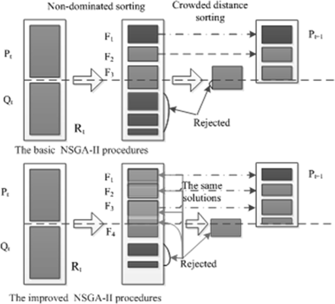

  

  An illustration of elite retention strategies

  As a comparison, for the same benchmark, the genetic manipulation of NSGA-II is the same as that of the adaptive weighting method described above. The difference is that in the process of binary selection, NSGA-II selects the best individual to enter the next generation according to the individual’s non-dominant level and crowding degree distance. For example, for individuals A and B, rank represents the non-dominant rank of the individual, and distance represents the crowding degree distance of the individual. If A_rank < B_rank or A_rank = B_rank and A_distance > B_distance, then solution A is better than solution B.

5.2.4 The Impact of Carbon Emissions on Enterprise Network Design

To study the impact of carbon emissions on enterprise logistics network design, this section conducts a sensitivity analysis of the issue from four aspects: CO₂ credits, ICP service coverage, ICP capacity, and CO₂ emission caps.

• (1) Sensitivity Analysis of CO₂ Credit Prices

Through a sensitivity analysis of the price of CO₂ credits, this section studies its impact on profits, CO₂ emissions, and the cost structure. The price of the CO₂ credit can take the values 0, 30, 60, 90, and 120. When the CO₂ credit price is increased from 0 to 120, profits and CO₂ emissions are reduced. This shows that given an increase in the CO₂ credit price, although the total amount of CO₂ emissions decreases, the total cost of emissions increases due to the increase in the CO₂ credit line. In addition to the increase in emission costs, fixed, rental, transportation, and inventory costs also increase, resulting in a decline in profits. Thus, as the CO₂ credit price increases, CO₂ emissions will decrease as the transportation route and duration shortens. This results in an increase in the number of CRCs and ICPS, with the collection period being prolonged; the corresponding construction, rental, and inventory costs will also increase. Furthermore, the longer the collection period of the ICP, the greater the cost of transportation. Therefore, the rise in the price of carbon credits increases the cost of the transportation mode and remanufacturing technology. The results show that if the credit for CO₂ is raised to 120, applying less environmentally friendly remanufacturing technologies will increase the remanufacturing emission cost. All solutions at the Pareto frontier in this section use the most environmental-friendly remanufacturing technologies. This also explains why an increase in the price of CO₂ credits is a good way to encourage investment in environmentally friendly technologies and promote a reduction in the overall CO₂ emissions of the reverse logistics network.

• (2) Sensitivity Analysis of Service Coverage

Based on the changes to the scope of services, we perform a sensitivity analysis on the model. The ICP services can take the values 25, 30, 35, and 40. When the service scope is 20 or 50, there is no feasible solution. The reason for this is that the scope of the service restrictions is too strict. The distance from the nearest ICP to customer channels still exceeds the maximum allowable distance. When the service scope is increased from 30 to 40, the number of initial infeasible solutions reduces from 185 to 94. While the minimum emissions reduce, the gap between the maximum and minimum emissions does not change significantly. The maximum and minimum profits also reduce, as does the gap between them. Thus, the average profit increases. This increase is due to a reduction in the total cost. As the scope of the service limit expands, the average number of open ICPs and CRCs is reduced, as is the collection period. This also reduces the construction, rental, and inventory costs. Moreover, with an increased scope of services, more appropriate ICPs and CRCs may be opened and the distance between the ICP and CRC is shortened. Thus, the cost of transportation is reduced with the expansion of the scope of service. These results show that enterprises must improve their scope of customer service. If service coverage is not the main factor affecting the number of returns, it is expected that the expanded service coverage will save costs. It is important to choose an appropriate service scope according to cost constraints and service requirements.

• (3) Sensitivity Analysis of ICP Capacity

The ICP capacity can take the values 200,300, 400, and 500. As the ICP capacity increases, CO₂ emissions and profits decrease. The reasons for this phenomenon are as follows. First, as the ICP capacity increases, fewer ICPs are required to satisfy the capacity constraint, thereby reducing the leasing cost. Second, an increase in ICP capacity also leads to an increase in its collection period. The longer the period of collection, the higher the inventory cost. Third, an increase in the ICP capacity and extension of the collection period led to an increase in the setup cost of ICPs. Fourth, the longer the collection period of the ICP, the lower the transport frequency from ICP to CRC, which implies lower CO₂ emissions. Thus, the emission cost is reduced. When the ICP capacity is increased from 200 to 300, the transportation costs decrease, but more crucially, the CO₂ emissions decrease. The increased setup and inventory costs are higher than the saved cost; thus, decreasing the total profit. The results show that an increase in ICP capacity helps to reduce the CO₂ emissions generated by the reverse logistics network but will lead to a reduction in profits.

• (4) Sensitivity Analysis of the CO₂ Emission Cap

The CO₂ emission cap in this section can take the values 10,000, 12,000, 14,000, and 16,000. With a relaxation of the cap on CO₂ emissions, CO₂ emissions and profits increase. A strict CO₂ cap will prompt enterprises to shorten the transportation distance and setup more CRCs. Relaxation of the CO₂ emissions cap reduces the setup cost of the CRC. Transportation branches and costs are reduced. With the relaxation of the CO₂ emission cap, investment in transportation methods and environmentally friendly remanufacturing technology is also decreased. It is also implied that with the given change in the CO₂ emission cap, the inventory and rental costs do not change significantly, which means that the strictness of the CO₂ emission cap also affects the promotion of reduction in CO₂ emissions.

5.3 Design of Waste Product Collection Channels

5.3.1 Design of Waste Product Collection Channels Regarding Enterprises’ Green Growth Model

The design of waste product collection channels is not only an expansion of the reverse value chain, but also of the whole process, including product design, manufacturing, selling, collection, and reuse, of waste products [16]. To achieve the objectives of the green growth model, enterprises need to reconstruct the existing value chain and business scope. The network redesign of the reverse value chain is an important part of the value chain reconstruction. The enterprise collects and harmlessly recycles the waste products through the collection channels, which effectively reduces environmental pollution by the waste products. Doing so simultaneously achieves the reuse of resources, improves resource efficiency and economic benefits, and finally realizes the goals of enterprises’ green growth model. Online and offline collaborations and the domination of waste product collection channels by different collectors together determine if the waste product collection market is in complete competition. This allows the construction of an important value chain network, combining forward and reverse value chains, for enterprises to implement enterprises’ green growth model.

5.3.2 Framework of Design of Waste Product Collection Channels

• (1) Different Collection Channels for Waste Products

Research on selection strategies for channels to collect waste products is primarily based on Savaskan et al. [17]. The model framework focuses on the efficiency, comparison, and selection of different recycling channels, such as manufacturers, retailers, and third-party collectors [18]. The core objective of this research branch is to develop an optimal collection strategy by comparing different collection channels. For example, Atasu et al. further studied the comparison of collection channels between manufacturers and retailers based on the aforementioned classical model [19], while De Giovanni et al. studied the simultaneous comparison of recovery efficiency among these three collectors [20]. On the basis of this, another branch of research considers collection cooperation among supply chain members.

• (2) Factors Influencing the Design of Waste Product Collection Channels

• (a) Competitive Factors in Collection Channels for Waste Products

Competition among collection channels affects their design. The competitive behavior of different collectors in the market, with their own collection channels, are primarily analyzed by using the Stackelberg game or completely static game theories, such as competition between the manufacturer and third-party collectors, competition between the manufacturer and retailer, competition between the retailer and third-party collectors, and competition among all three collectors. Additionally, some studies mentioned more specific competition within the same collection channels, such as competition between the same value chain members as multiple retailers, multiple collectors, and multiple manufacturers in the value chain. Moreover, Han et al. have studied the collection competition between different supply chains where competition and integration models are more complicated but are more in line with industrial supply chain integration [21].

• (b) Consumer Factors in Waste Product Collection Channels

In the context of competition, consumers’ preferences for collection channels also affect enterprises’ design of collection channels for waste products. These include economic incentives, willingness to pay for new or refined products, environmental awareness, and perception of the convenience level of collection channels. Most previous research has focused on how to recycle products, e.g., centralized collection, manufacturer collection, or retailer collection, and how to price products to improve collection efficiency. Feng et al. studied the advantages and disadvantages of a single traditional collection channel, a single online collection channel, and a centralized and decentralized mixed dual collection channel to examine consumer preferences for online collection channels [22]. Recently, an increasing number of studies have focused on the factors influencing consumers’ return preferences from a psychological perspective. Simpson et al. have used empirical methods to discuss how psychological ownership affects consumers’ the return behavior of consumers for reusable products [23].

• (3) Different Reuse Technologies in Enterprises’ Green Growth Model

To approach a green closed-loop supply or value chain, enterprises should remanufacture waste products after collection for technical, local regulatory, and economic considerations. Using waste product recovery options such as remanufacturing [24] and recycling [25], enterprises can put collected waste products back into the forward production process of the closed-loop supply chain to achieve resource reuse and environmental protection. Waste products should be remanufactured to achieve the identical functionality and appearance of new products, and then be marketed as new products. Collectors that use remanufacturing often use usable parts from waste products to create new products and services, thereby reducing the product costs.

Different reuse technologies exhibit different features. First, when compared with recycling, although remanufacturing brings higher economic benefits, it also has higher technological, capital, and process thresholds. Typically, only manufacturers with certain production and operational advantages can undertake remanufacturing. Recycling, in turn, makes a profit by extracting raw materials, such as precious metals and plastics, from the waste products, or by receiving a subsidy for selling the waste product to the upstream of the value chain. Second, different reuse methods for waste products have different resource efficiencies with remanufacturing having a relatively higher resource effeciency than others.

5.3.3 Model of Waste Product Collection Channel Regarding Different Reuse Technologies

Currently, remanufacturing and recycling are the main environmental protection technologies for collecting waste products and integrating them into the value chain so that the enterprises’ green growth model can help enterprises improve their green level and economic benefits. Generally speaking, remanufacturing has higher requirements for the technology, process, equipment, and human resources of enterprises, in addition to a certain threshold for the industry. By contrast, other collectors who are not original manufacturers have difficulty in remanufacturing, which makes recycling a smarter choice for these companies. However, the lower resource efficiency of recycling results in a lower green level of the supply chain. At the same time, the competition model in which different collectors choose different reuse technologies (manufacturers choose remanufacturing, whereas retailers choose recycling) is particularly significant in the real industry. Although non-manufacturer collectors can also profit from recycling, enterprises must consider the lower resource efficiency and potential secondary pollution caused by recycling.

The model of waste product collection channels regarding different reuse technologies mainly studies the competition mechanism between manufacturers and retailers that adopt different reuse technologies of waste products in Fig. 5.11. This section also refines and proposes models of waste product collection channels based on different reuse technologies.

Fig. 5.11

Model framework for waste-product collection channels regarding different reuse options

• (1) Model of Waste Product Collection Channel Based on Recycling

Let $\tau_i (i = C,M,R)$ denote the collection rate, where C, M, and R are the supply chain alliance, manufacturer, and retailer of the centralized model, respectively. Let $c_i$ denote the consumer perceived inconveniences of the collection channels from the centralized alliance, manufacturer, and retailer. Let $s_i$ denote the level of service provided to consumers through the different channels. Let $\pi_i$ denote the total profits of the alliance, the manufacturer, and the retailer. Note that this section defines $c_m$ as the manufacturer’s cost of the new product, while $c_r$ is the remanufacturing cost; thus, $c_m > c_r$.

For the retailer, k represents the basic surplus value extracted from the reused products and $k \cdot \tau_R$ is the total profit of the retailer from collection activities.

• (2) Model of Waste Product Collection Channel Based on Remanufacturing

For manufacturers, there are two ways of production: making new products from new raw materials or making new products from collected products. For the manufacturer and supply chain alliance, the collection rate is the proportion $\tau_i$ of all new products that can be remanufactured at the unit cost $c_r$. Thus $1 - \tau_i$ is the proportion of all new products produced using new raw materials and components at the unit cost $c_m$. Therefore, the combined cost of the alliance or manufacturer can be expressed as $c_m (1 - \tau_i ) + c_r \tau_i$. Further, setting e ($e = c_m - c_r$) as the difference between the cost of the new product and that of the remanufactured product, we have

$$ c_m (1 - \tau_i ) + c_r \tau_i = c_m - e\tau_i $$

• (3) Model of Waste Product Collection Channels Based on Different Reuse Technologies

The model of different reuse technologies for waste product collection channels is based on the long-term operational stability of the single cycle model; thus, the model does not consider inventory, transportation, or delivery, while also assume that the collection and recovery costs and product quality are fixed. This model focuses on the analysis of the competitive and behavioral factors. Assume a linear relationship between the demand for new products and the selling price set by retailers, that is $d = \alpha - \beta p$. In addition, assume a Stackelberg game between the retailer and manufacturer, with the manufacturer as the leader.

In a highly competitive collection market, the consumer-perceived collection inconveniences are $c_R$ and $c_M$, where $c_R = 1 - s_R$ and $c_M = 1 - s_M$. This model assumes that the collection value of the consumers is uniformly distributed as in $v \sim U(0,1)$. According to the basic assumption, the more inconvenient consumers feel when returning used products, the less utility they receive from collection activities. The collection utility functions for consumers are as follows:

$$ \left\{ \begin{gathered} U_R (v,c_R ) = v - c_R \hfill \\ U_M (v,c_M ) = \theta v - c_R \hfill \\ \end{gathered} \right. $$

In particular, $\theta \in (0,1)$ indicates consumers’ negative influence on the collection channel of manufacturers. As retailers can easily interact and directly communicate with consumers through the retail network, consumers’ initial impression of the manufacturer’s collection activities is worse than that of the retailers. Consumers may be faced with four recycling utility functions: if $U_R > U_M > 0$, the retailer collects all used products; if $U_M > U_R > 0$, the manufacturer collects all; if $U_M < 0,U_R < 0$, consumers refuse any returning; and if $U_M = U_R > 0$, consumers will choose either channel for returning. Therefore, the collection rates are

$$ \begin{gathered} \tau_R = \left\{ \begin{gathered} 1 - \frac{s_M - s_R }{{1 - \theta }},if\frac{1 - s_M }{\theta } \le 1 - s_R \hfill \\ s_R ,Otherwise \hfill \\ \end{gathered} \right. \hfill \\ \tau_M = \left\{ \begin{gathered} \frac{s_M - \theta s_R - (1 - \theta )}{{\theta (1 - \theta )}},if\frac{1 - s_M }{\theta } \le 1 - s_R \hfill \\ 0,Otherwise \hfill \\ \end{gathered} \right. \hfill \\ \end{gathered} $$

On this basis, according to the model structure in Fig. 5.11, the profit functions of the manufacturers and retailers are:

$$ \begin{gathered} \pi_M = (w - c_m + e\tau_M )(\alpha - \beta p) - \frac{A}{2}s_M^2 \hfill \\ \pi_R = (p - w)(\alpha - \beta p) + k\tau_R - \frac{A}{2}s_R^2 \hfill \\ \end{gathered} $$

where w is the wholesale price and A is the cost index of service level.

By backward induction:

• (a) When $\frac{c_M }{\theta } > c_R$:

  $$ w_1^{*} = \frac{\alpha + c_m \beta }{{2\beta }} $$
  $$ s_{M1}^{*} = 0 $$
  $$ p_1^{*} = \frac{3\alpha + c_m \beta }{{4\beta }} $$

• (b) When $\frac{c_M }{\theta } \le c_R$:

The retailer’s optimal collection investment and selling strategies are:

$$ \left\{ {\begin{array}{*{20}c} {s_{R2}^{*} = \frac{ku}{A}} \\ {p_{D2}^{*} = \frac{\alpha }{2\beta } + \frac{ - \alpha \beta e^2 u^2 v^2 + 2\beta keu^2 + 2A\beta ev + 2A\alpha + 2A\beta c_m }{{2\beta \left( {4A - \beta e^2 u^2 v^2 } \right)}}} \\ \end{array} } \right. $$

The manufacturer’s optimal collection investment and wholesale pricing decisions are:

$$ \left\{ {\begin{array}{*{20}c} {s_{M2}^{*} = \frac{{euv\left( {\beta eku^2 + A\beta ev + A\beta c_m - A\alpha } \right)}}{{A\left( {\beta e^2 u^2 v^2 - 4A} \right)}}} \\ {w_{D2}^{*} = \frac{ - \alpha \beta e^2 u^2 v^2 + 2\beta keu^2 + 2A\beta ev + 2A\alpha + 2A\beta c_m }{{\beta \left( {4A - \beta e^2 u^2 v^2 } \right)}}} \\ \end{array} } \right. $$

The collection rates of manufacturers and retailers are:

$$ \tau_{R2}^{*} = 1 - us_{M2}^{*} + us_{R2}^{*} = \frac{ku^2 }{A} + 1 + \frac{{eu^2 v\left( {\beta eku^2 - A\alpha + A\beta c_m + A\beta ev} \right){ }}}{{A\left( {\beta e^2 u^2 v^2 - 4A} \right)}} $$

$$ \tau_{M2}^{*} = uvs_{M2}^{*} - us_{R2}^{*} - v = \frac{{eu^2 v^2 \left( {\beta eku^2 - A\alpha + A\beta c_m + A\beta ev} \right)}}{{A\left( {\beta e^2 u^2 v^2 - 4A} \right)}} - v - \frac{ku^2 }{A} $$

And the total collection rate of reverse channels is:

$$ \tau_{D2}^{*} = \tau_{R2}^{*} + \tau_{M2}^{*} = 1 - v + \frac{{euv^2 \left( {\beta eku^2 + A\beta ev + A\beta c_m - A\alpha } \right)}}{{A\left( {\beta e^2 u^2 v^2 - 4A} \right)}} $$

The analysis of the model’s results shows that, first, collection competition cannot improve manufacturer-led collection efficiency. Although the contract mechanism can achieve optimal recovery efficiency, it still has some shortcomings. Channel discrimination has limited influence on the collection rate and decision-making strategy in a decentralized supply chain. Second, retailers are always willing to compete in recycling, but there is no obvious relationship between the low-cost advantage of remanufacturing and collection efficiency. Thus, the investment level of manufacturers is not high. Finally, retailers’ participation in collection greatly increases competition for collection, leading to a decline in collection efficiency. With an increase in investment in collection channels, retailers gradually lose the benefits of the consumer’s channel preference. Therefore, collection competition reduces the efficiencies of manufacturers’ collection and supply chain resources. Likewise, an elevated level of consumer channel discrimination reduces both total collection efficiency and resource efficiency. Enterprises, such as manufacturers and retailers, should realize enterprises’ green growth model with economic, environmental, and social benefits through a value chain reconstruction according to their practical situation.

5.4 Summary

This chapter analyzes and introduces the basic framework of network design and relevant methods, and subsequently proposes two patterns to help enterprises implement the network design of enterprises’ green growth model: network design considering carbon emissions and design of waste product collection channels. The network designs from both perspectives reveal how to improve green and growth levels. First, to reduce the network operation costs and carbon emissions, a network design that considers carbon emissions is focused on the entire network to achieve a more efficient value chain network through a series of optimization methods. Second, to maximize the collected core quantities, the design of waste product collection channels focuses on suitable collection mechanisms, interactions of different value chain members’ decisions, and a reverse channel collection network regarding different waste product reuse technologies.

References

Peppard, J., & Rylander, A. (2006). From value chain to value network: Insights for mobile operators. European Management Journal, 24(2–3), 128–141.
Farahani, R., Rezapour, S., Drezner, T., & Fallah, S. (2014). Competitive supply chain network design: An overview of classifications, models, solution techniques and applications. Omega, 45, 92–118.
Rad, R. S., & Nahavandi, N. (2018). A novel multi-objective optimization model for integrated problem of green closed loop supply chain network design and quantity discount. Journal of Cleaner Production, 196, 1549–1565.
Prakash, S., Kumar, S., Soni, G., Jain, V., & Rathore, A. P. S. (2020). Closed-loop supply chain network design and modelling under risks and demand uncertainty: An integrated robust optimization approach. Annals of Operations Research, 290(1), 837–864.
Farshbaf-Geranmayeh, A., Taheri-Moghadam, A., & Torabi, S. A. (2020). Closed loop supply chain network design under uncertain price-sensitive demand and return. Infor, 58(4), 606–634.
Ozkan, O., & Kilic, S. (2019). A Monte Carlo Simulation for reliability estimation of logistics and supply chain networks. IFAC-PapersOnLine, 52(13), 2080–2085.
Nouira, I., Hammami, R., Frein, Y., & Temponi, C. (2016). Design of forward supply chains: Impact of a carbon emissions-sensitive demand. International Journal of Production Economics, 173, 80–98.
Muhammad, S., & Long, X. (2021). Rule of law and CO2 emissions: A comparative analysis across 65 belt and road initiative (BRI) countries. Journal of Cleaner Production, 279, 123539.
Teng, F., & Wang, P. (2021). The evolution of climate governance in China: Drivers, features, and effectiveness. Environmental Politics, 30(sup1), 141–161.
Choi, B., Luo, L., & Shrestha, P. (2021). The value relevance of carbon emissions information from Australian-listed companies. Australian Journal of Management, 46(1), 3–23.
Sovacool, B. K., Martiskainen, M., Hook, A., & Baker, L. (2019). Decarbonization and its discontents: A critical energy justice perspective on four low-carbon transitions. Climatic Change, 155(4), 581–619.
Zhang, W., Li, J., Li, G., & Guo, S. (2020). Emission reduction effect and carbon market efficiency of carbon emissions trading policy in China. Energy, 196, 117117.
Wang, Q., & Su, M. (2020). Drivers of decoupling economic growth from carbon emission–an empirical analysis of 192 countries using decoupling model and decomposition method. Environmental Impact Assessment Review, 81, 106356.
Reddy, K. N., Kumar, A., Sarkis, J., & Tiwari, M. K. (2020). Effect of carbon tax on reverse logistics network design. Computers & Industrial Engineering, 139, 106184.
Chen, X., & Lin, B. (2021). Towards carbon neutrality by implementing carbon emissions trading scheme: Policy evaluation in China. Energy Policy, 157, 112510.
He, Q., Wang, N., Yang, Z., He, Z., & Jiang, B. (2019). Competitive collection under channel inconvenience in closed-loop supply chain. European Journal of Operational Research, 275(1), 155–166.
Savaskan, R. C., Bhattacharya, S., & Van Wassenhove, L. N. (2004). Closed-loop supply chain models with product remanufacturing. Management Science, 50(2), 239–252.
Xiao, Y. (2017). Choosing the right exchange-old-for-new programs for durable goods with a rollover. European Journal of Operational Research, 259(2), 512–526.
Atasu, A., Toktay, L. B., & Van Wassenhove, L. N. (2013). How collection cost structure drives a manufacturer’s reverse channel choice. Production and Operations Management, 22(5), 1089–1102.
De Giovanni, P., & Zaccour, G. (2014). A two-period game of a closed-loop supply chain. European Journal of Operational Research, 232(1), 22–40.
Han, X., Wu, H., Yang, Q., & Shang, J. (2016). Reverse channel selection under remanufacturing risks: Balancing profitability and robustness. International Journal of Production Economics, 182, 63–72.
Feng, L., Govindan, K., & Li, C. (2017). Strategic planning: Design and coordination for dual-recycling channel reverse supply chain considering consumer behavior. European Journal of Operational Research, 260(2), 601–612.
Simpson, D., Power, D., Riach, K., & Tsarenko, Y. (2019). Consumer motivation for product disposal and its role in acquiring products for reuse. Journal of Operations Management, 65(7), 612–635.
Abbey, J. D., Meloy, M. G., Guide, V. D. R., Jr., & Atalay, S. (2015). Remanufactured products in closed-loop supply chains for consumer goods. Production and Operations Management, 24(3), 488–503.
Agrawal, V. V., Atasu, A., & Van Wassenhovec, L. N. (2019). New opportunities for operations management research in sustainability. Manufacturing & Service Operations Management, 21(1), 1–12.
Author information
Authors and Affiliations
Corresponding author
Rights and permissions
Copyright information
© 2022 The Author(s), under exclusive license to Springer Nature Singapore Pte Ltd.
About this chapter
Cite this chapter
Zhang, M., Yuchi, Q., Wang, N., He, Q. (2022). Network Design in Enterprises’ Green Growth Model. In: Enterprises’ Green Growth Model and Value Chain Reconstruction. Springer, Singapore. https://doi.org/10.1007/978-981-19-3991-4_5
Download citation
DOI: https://doi.org/10.1007/978-981-19-3991-4_5
Published:
Publisher Name: Springer, Singapore
Print ISBN: 978-981-19-3990-7
Online ISBN: 978-981-19-3991-4
eBook Packages: Economics and FinanceEconomics and Finance (R0)