Optimization of System Reliability with Time-Dependent Reliability Components in Imprecise Environment Using Hybridized QPSO

Abstract

To design reliable systems, the optimization of system reliability (SR) is a highly concerned topic in the engineering design and industry. The reliability optimization aims to develop a reliable system with higher reliability to perform satisfactorily under certain conditions and up to a specified period. This chapter considers the redundancy allocation problem as a highly non-linear and integer programming constrained optimization problem. To cope up with reality with unpredictability, we desire to consider the reliabilities of the time-dependent components that lead to a reliable time-dependent system. Further, to incorporate the fluctuating behaviour of the system's controlling parameters and uncertainty of the situations of the environment in which the system is operated, we developed the fuzzy model. As the problem is combinatorial and highly non-linear, we developed and implemented the hybridized metaheuristic technique derived by combining QPSO, a variant of particle swarm optimization, and the Big-M penalty technique to find the solution. The crisp and fuzzy (triangular and pentagonal) models are solved, and the comparative studies are presented. The statistical computations and the sensitivity studies of the HQPSO parameters are also presented corresponding to the numerical experiments.

1 Introduction

During the last few decades, many researchers have shown their keen interest in the study of reliability optimization. A wide area of applications of reliability design is observed such as engineering and industry, machine design and productions, including networking communications and transportations, etc. Also, industrialists and machine designers have been showing their interest in reliability theory and practice as it has many practical applications. Reliability analysis is an important part of many developmental works in system designing, communication systems, infrastructure development, etc. System reliability is practically the probability of successful performance of a system up to a given period under some predetermined conditions. The reliability components are taken with fixed values in most of the works reported in the literature. However, it is more realistic to consider the reliability of a system as a function of time since it undoubtedly decreases with time. In this research area, some researchers have presented such a genuine attempt in the literature review of reliability optimization. The reliability practitioners always desire to maximize the system reliability and the considered system's lifetime under certain constraints.

Several types of reliability optimization problems have been designed and solved in the literature such as Redundancy Allocation Problem (RAP), Reliability Redundancy Allocation Problem (RRAP), etc. Most attempts are found in redundancy allocation problems. In this work, our main target is to consider the RAP type of problem in which redundant components are allocated with regard to some constraints to optimize the system reliability. The renowned researchers like, Tillman et al. (1980), Sun and Li (2002), Mahapatra and Roy (2011), Mahato et al. (2020), Garg et al. (2014), Gupta et al. (2009), Mahato et al. (2013), Sahoo et al. (2013), etc. have reported important contributions in the literature. The heuristic technique in optimal reliability allocation reported by Nakagawa and Nakashima (1977), the fuzzy environment is used reliability optimization by Chen (1977), the reduced gradient method utilized by Hwang et al. (1979), a detailed study of the optimization of the reliability of a system is done by Tillman et al. (1980), the surrogate constrained algorithm is used by Nakagawa and Miyazaki (1981). The remarkable researchers such as Chern and Jan (1986), Misra (1986), Park (1987), Misra and Sharma (1991), Huang (1996), Sung and Cho (2000), Kuo et al. (2001) Sun and Li (2002), Mahapatra and Roy (2006, 2009, 2011), Gupta et al. (2009), Bhunia et al. (2010), Sahoo et al. (2010), Bhattacharyee et al. (2021), etc. are notable in the field of reliability optimization.

The uncertainty concepts such as interval, fuzzy, and intuitionistic fuzzy are introduced and studied by many researchers in the reliability analysis. These studies gave a new direction in the study of reliability models. These models are proved to be more realistic in terms of real-life phenomena. The concepts of generalized fuzzy number (Mahapatra and Roy 2011, 2012; Garg 2013; Mahato et al. 2013; Sahoo et al. 2013, 2014; Mahato et al. 2020), interval number (Bhunia and Sahoo 2011; Mahapatra and Roy 2012; Sahoo et al. 2012; Mahato et al. 2012), intuitionistic fuzzy (Garg 2013; Garg and Rani 2013; Garg et al. 2014; Garg 2015; Jamkhaneh 2017, Bhattacharyee et al. 2021) are introduced and studied in reliability theory.

The use of soft computing techniques is observed to have a great impact on reliabity optimization. Usually, the designed problems are found to be highly non-linear combinatorial problems and the analytical solutions are very difficult. So to handle such problems several soft computing algorithms are designed and implemented to solve reliability optimization problems. Soft computing techniques like, GA, PSO, and ABC, etc. are proved to be highly effective in finding the optimal reliability for any type of reliability optimization problems. The works of several researchers like, Garg (2013), Garg and Rani (2013), Khalili-Damghani et al. (2013), Garg et al. (2014a, b), Sahoo et al. (2012, 2013, 2014), Garg (2015, 2016, 2017), Gupta et al. (2009), Mahato et al. (2013, 2020), Bhattacharyee et al. (2021) are worth mentioning. The list is not exhaustive but there are lots of researchers who have developed and utilized several algorithms to solve the problems of reliability maximization.

The time-dependent reliability models are also very much relevant in reliability theory and practice. To make the models more realistic, the reliabilities of the components should be considered to be a function of time. Only a few researchers have designed the reliability models with time-dependent reliability. The works, in this regard, of Mori and Ellingwood (1993), Hamadani and Khorshidi (2013), Ganzalezet al. (2015), Hu and Mahadevan (2015), Mourelatos et al. (2015), Wang et al. (2015), Zhu and Zhifu (2016), Mostafa (2017), Ahmadivala et al. (2019), Zafar and Wang (2020), Bhattacharyee et al. (2021), etc. are noteworthy.

This chapter's main goal is to consider the reliable system having time-varying component reliabilities and the impreciseness of the environments. We have considered here the component’s reliabilities to follow exponentially decreasing function of time. So, the reliability model developed here becomes time-dependent. This work has included the impreciseness in terms of triangular fuzzy and pentagonal fuzzy numbers to handle the fluctuating situations, which certainly looks to be more realistic. Hence, we have three models including the two imprecise models, viz., the crisp model, the triangular fuzzy model, and the pentagonal fuzzy model. We developed a new soft computing algorithm to solve the problems. The newly proposed algorithm is named Hybridized Quantum-behaved PSO (HQPSO) which is a variant of PSO involving the Big-M penalty technique.

Organization of the Chapter

Section 1		Introduction
Section 2		Research Gaps
Section 3		Notation and Assumptions
Section 4		Mathematical Foundations
Subsection 4.1		Relevent Definitions
Subsection 4.2		Method of Defuzzification of Fuzzy Numbers
Section 5		Problem Formulation
Subsection 5.1		The Crisp Model
Subsection 5.2		The Fuzzy Models
Section 6		Solution Procedure
Subsection 6.2		Particle Swarm Optimization
Subsection 6.3		Quantum behaved Particle Swarm Optimization (QPSO)
Subsection 6.4		Proposed Hybridized QPSO
Section 7		Numerical Experiments
Section 8		Result Discussions
Section 9		Acknowledgements

2 Research Gaps

It is clearly to be noted from the existing literature that most of the reliability optimization problems focused on precise environments. Some researchers have recently presented their research on imprecise environments that include interval, fuzzy, intuitionistic fuzzy, stochastic, and a mixture of these. Few works in this area are found to attempt the problems on reliability optimization using GA, PSO, hybridized PSO, ABC algorithms, Cuckoo search algorithm, and other heuristic algorithms. Moreover, in most of the works related to our paper, the reliability components are of constant values and only a few are observed to consider these as time-varying functions. A few works are also found to consider the machine design life as the objective function, and the others have taken system reliability or the cost function as the objective function.

Again, the problem's constraints are handled in several ways; only our research group in this field has incorporated the Big-M penalty method. Thus, we have been motivated eagerly to formulate a problem in reliability studies which has the machine design life as the objective function, the reliability component as exponentially decreasing functions of time, utilize the Big-M penalty technique to tackle the constraints. We use Simpson’s 1/3 rule to handle the integration to get the machine design life from system reliability function and develop a hybridized Quantum-behaved Particle Swarm Optimization due to Big-M penalty method.

3 Notation and Assumptions

Throughout the chapter, we use the symbols described below. Also, the necessary assumptions to formulate the problem under consideration are given below.

3.1 Notation

Symbols		Meanings
$\stackrel{\sim }{P, }\widehat{P}$		Triangular and Pentagonal fuzzy number respectively
${\mu }_{\tilde{P }}\left(x\right),{\mu }_{\widehat{P}}\left(x\right)$		Membership function of x $\in X$ w.r.t. $\tilde{P },\widehat{P}$ respectively
$Cr1\left(\tilde{P }\right),Cr2(\widehat{P})$		Defuzzified value of the fuzzy number $\tilde{P },\widehat{P}$ respectively
$u=\left({u}_{1},{u}_{2},\dots ,u\right)$		Redundancy vector (decision variable)
${R}_{1}\left(u,\lambda ,t\right)$,${\tilde{R }}_{2}\left(u,\stackrel{\sim }{\lambda },t\right),$ ${\widehat{R}}_{3}\left(u,\widehat{\lambda },t\right)$		System reliability in crisp, triangular fuzzy and pentagonal fuzzy forms respectively
${M}_{1}\left(u,\lambda ,{M}_{T}\right), {\tilde{M }}_{2}\left(u,\stackrel{\sim }{\lambda },{M}_{T}\right),{\widehat{M}}_{3}(u,\widehat{\lambda },{M}_{T})$		MDL in crisp, triangular fuzzy and pentagonal fuzzy forms respectively
${g}_{1j}\left(u\right)$, ${\tilde{g }}_{2j}\left(u\right), {\widehat{g}}_{3j}\left(u\right)$		Constraints usability functions in crisp, triangular fuzzy and pentagonal fuzzy environments
${b}_{1j}$,${\tilde{b }}_{2j},{\widehat{b}}_{3j}$		Availability of resources of j-th constraint in crisp, triangular fuzzy and pentagonal fuzzy environments
${l}_{1i},{l}_{2i}$		Lower bound and upper bound of ${u}_{i}$
$S_{size}$		Swarm size in QPSO
${f(p}_{i})$		Value of fitness function of i-th particle in its best position
$m_{i}^{(z)}$		Mean best position of j-thcomponent at z-th iteration
$m^{(z)}$		Mean best position vector at z-th iteration
$x_{ij}^{(z)}$ :		The position of i-thparticle in the j-th swarm at z-th iteration
$A_{ij}^{(z)}$		Local attractor of the j-th component of the i-th particle at z-th iteration
Mg		Maximum number of generations
n		Dimension of the variables
$F_{R}$		Feasible region

3.2 Assumptions

To develop our proposed model, we have careful into consideration of the assumptions given here:

• (i) The proposed system is a series–parallel system.

• (ii) At a particular stage, the subsystem contains identical components.

• (iii) Without any repair, the redundancies are always active.

• (iv) Reliability of each component is an exponentially decreasing function of time.

• (v) The MDL function is defined as the integral of system reliability.

• (vi) Component failure in each subsystem might not be tantamount to the system to its failure.

• (vii) Throughout all environments, the control parameters are well known, viz. crisp and fuzzy (triangular and pentagonal).

• (viii) Fuzzy numbers (triangular and pentagonal) are of linear type.

4 Mathematical Foundations

4.1 Relevant Definitions

Definition 4.1:

The fuzzy set is the pair (x,${\mu }_{\tilde{P }}(x)$), where x $\in X$ and ${\mu }_{\tilde{P }}(x)$:X → [0, 1], X being the universe of discourse and it is represented as $\tilde{P }$={(x,${\mu }_{\tilde{P }}(x)$): x $\in$ X}, where ${\mu }_{\tilde{P }}(x)$ denotes the membership function of x $\in X$ w.r.t. $\tilde{P }$.

Definition 4.2:

The fuzzy set $\tilde{P }$ becomes convex iff $\mu_{{\tilde{P}}} (\lambda x_{1} + (1 - \lambda )x_{2} ) \ge \min \{ \mu_{{\tilde{P}}} (x_{1} ),\mu_{{\tilde{P}}} (x_{2} )\} ,$ for all $x_{1} ,x_{2} \in X$, where $\lambda \in [0,1]$.

Definition 4.3:

The fuzzy set $\tilde{P }$ becomes normal if $\mu_{{\tilde{P}}} (x) = 1$, for some x $\in X$.

Definition 4.4:

A fuzzy set becomes a fuzzy number provided it is (Fig. 1).

Fig. 1

General fuzzy number

• (i) Normal

• (ii) convex

The membership function of a fuzzy number $\tilde{P }$ can be described as

$$\mu_{{\tilde{P}}} (x) = \left\{ \begin{gathered} l{(}x{), }p_{1} \le x < p_{2} \hfill \\ 1, \, p_{2} \le x \le p_{3} \hfill \\ u{(}x{), }p_{3} < x \le p_{4} \hfill \\ 0,\,{\text{ otherwise}}. \hfill \\ \end{gathered} \right.\,\,\,\,$$

l(x) and u(x) being the left and right shape functions, respectively.

Definition 4.5: Linear Triangular Fuzzy Number (LTFN)

An LTFN $\tilde{P}$ is represented by the triplet $(p_{1} ,p_{2} ,p_{3} )$ and can be defined by the continuous membership function $\mu_{{\tilde{P}}} (x):X \to [0,1]$ as follows:

$$\mu_{{\tilde{P}}} (x) = \left\{ \begin{gathered} \frac{{x - p_{1} }}{{p_{2} - p_{1} }}\,\,\,\,\,\,\,\,{\text{if}}\,p_{1} \le x \le p_{2} \hfill \\ 1\,\,\,\,\,\,\,\,\,\,\,\,\,\,\,\,\,\,\,\,\,\,{\text{if}}\,x = p_{2} \,\,\,\,\,\,\,\, \hfill \\ \frac{{p_{3} - x}}{{p_{3} - p_{2} }}\,\,\,\,\,\,\,\,{\text{if}}\,p_{2} \le x \le p_{3} \hfill \\ 0\,\,\,\,\,\,\,\,\,\,\,\,\,\,\,\,\,\,\,\,\,{\text{otherwise}}{.} \hfill \\ \end{gathered} \right.\,\,\,\,$$

Definition 4.6: Linear Pentagonal Fuzzy Numbe (LPtFN)

A fuzzy pentagonal number $\widehat{P}$= (${p}_{1}$,${p}_{2}$,${p}_{3}$,${p}_{4}$,${p}_{5}$) satisfies the conditions given below:

• (1) it has the continuous membership function ${\mu }_{\widehat{P}}\left(x\right)$ in [0,1]

• (2) the membership function ${\mu }_{\widehat{P}}\left(x\right)$ is strictly non-decreasing in [${p}_{1}$,${p}_{2}$] and [${p}_{2}$, ${p}_{3}$]

• (3) the membership function ${\mu }_{\widehat{P}}\left(x\right)$ is strictly non-increasing in [${p}_{3}$, ${p}_{4}$] and [${p}_{4}$, ${p}_{5}$] (Figs. 2 and 3)

  Fig. 2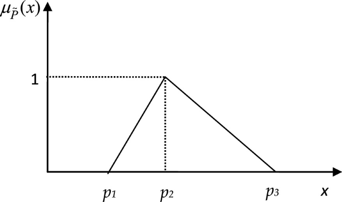

  

  Linear triangular fuzzy number

  Fig. 3

  

  Linear pentagonal fuzzy number

4.2 Method of Defuzzification of Fuzzy Number

There are several methods of defuzzification available in the literature. The most commonly used technique for defuzzification of a fuzzy number is the centre of area (COA) method.

Let the fuzzy number $\tilde{P }$ has a continuous membership function ${\mu }_{\tilde{P }}\left(x\right)$ then the COA formula for crispification is defined as follows (Mahato and Bhunia 2016).

$Cr1\left(\tilde{P }\right)= \frac{\int {\mu }_{\tilde{P }}\left(x\right)xdx}{\int {\mu }_{\tilde{P }}\left(x\right)dx}$.

4.2.1 Crispification Formula for Linear Triangular Fuzzy Number

The crispification formula for Linear Triangular Fuzzy Number $\tilde{P }=({p}_{1},{p}_{2},{p}_{3})$ can be defined as (Mahato and Bhunia 2016)

$Cr1(\tilde{P })$ = (${p}_{1}+{p}_{2}+{p}_{3}$)/3.

Example 4.1:

For $\tilde{P }=\left(\mathrm{2,3},4\right),{p}_{1}=2,{p}_{2}=3,{p}_{3}=4$, so

$Cr1(\tilde{P })$ = $\frac{1}{3}$(${p}_{1}+{p}_{2}+{p}_{3}$)

 = $\frac{1}{3}$($2+3+4$)

 = 3

Example 4.2:

For $\tilde{P }=(\mathrm{1.6,2.9,3.8}){p}_{1}=1.6,{p}_{2}=2.9,{p}_{3}=3.8$ and so

$Cr1(\tilde{P })$ = $\frac{1}{3}$(${p}_{1}+{p}_{2}+{p}_{3}$)

 = $\frac{1}{3}$($1.6+2.9+3.8$)

 = 2.7666666667

4.2.2 Crispification Formula for Linear Pentagonal Fuzzy Number

The crispification formula for Linear Pentagonal Fuzzy Number $\widehat{P}$= (${p}_{1}$,${p}_{2}$,${p}_{3}$,${p}_{4}$,${p}_{5}$) is defined as (Mahato and Bhunia 2016)

$Cr2(\widehat{P}$) = $\frac{{p}_{5}^{2}+{p}_{4}^{2}+{p}_{5}{p}_{4}-{p}_{1}{p}_{2}-{p}_{2}^{2}-{p}_{1}^{2}}{3({p}_{5}+{p}_{4}-{p}_{2}-{p}_{1})}$

Example 4.3:

For $\widehat{P}=\left(\mathrm{1,2},\mathrm{3,4},6\right),{p}_{1}=1,{p}_{2}=2,{p}_{3}=3$, ${p}_{4}$ = 4, ${p}_{5}$ = 6 and so

$Cr2(\widehat{P}$) = $\frac{{p}_{5}^{2}+{p}_{4}^{2}+{p}_{5}{p}_{4}-{p}_{1}{p}_{2}-{p}_{2}^{2}-{p}_{1}^{2}}{3({p}_{5}+{p}_{4}-{p}_{2}-{p}_{1})}$

 = 3.2857142857

Example 4.4:

For $\widehat{P}=(\mathrm{2.5,3.3,4.4,5.8,6.4})$, ${p}_{1}=2.5,{p}_{2}=3.3,{p}_{3}=4.4$, ${p}_{4}$ = 5.8, ${p}_{5}$ = 6.4 and so

$Cr2(\widehat{P}$) =$\frac{{p}_{5}^{2}+{p}_{4}^{2}+{p}_{5}{p}_{4}-{p}_{1}{p}_{2}-{p}_{2}^{2}-{p}_{1}^{2}}{3({p}_{5}+{p}_{4}-{p}_{2}-{p}_{1})}$  = 4.496354

5 Problem Formulation

This section covers the formulation of a series–parallel reliability redundancy allocation problem using the fact that the components have time-dependent reliabilities (Bhattacharyee et al. 2021). It is supposed that the reliability components obey exponential distributions, leading to the reliability of the system being time-dependent.

Moreover, we are inspired for considering the mission design life and desire to get the maximum value of the system reliability with a proper choice of the redundancy allocation vector. Evidently, it is better not to take the controlling parameters as fixed numbers by some deterministic rule but to consider these as imprecise numbers to retain the reliable system's unpredictable nature. The parameters’ estimated values cannot be predicted precisely due to the reliability system's fluctuating character. This unpredictable situation can be handled by considering the impreciseness in terms of fuzzy, intuitionistic fuzzy, interval, stochastic, or combination. In the fuzzy approach, we need to know the membership function for a given fuzzy number, while for an intuitionistic fuzzy approach, we should know both the membership function and the non-membership function. For the interval method, the parameters are taken as closed intervals. Some known probability distributions are taken in the stochastic approach. In this work, we assume the impreciseness/vagueness in the form of fuzzy numbers (TFN and PtFN). Thus, depending upon the nature of the controlling parameters, we develop three models corresponding to the series-parallelsystem (Fig. 4).

Fig. 4

Series–parallel system with n-stages

5.1 The Crisp Model

To solve the redundancy allocation problem (RAP) with time-varying reliability, we considered the reliability component following the exponential failure rate and time-dependent component reliability function. We have considered a system with n subsystems connected in series, and each subsystem consists of ${u}_{i}$($i=\mathrm{1,2},\dots ,n$) the number of active redundant components which are identical.

Let the failure density function be ${f}_{i}\left(t\right)={\lambda }_{i}{e}^{-{\lambda }_{i}t}$ and the reliability function of each component of the i-th subsystem be ${r}_{i}\left(t\right)={e}^{-{\lambda }_{i}t}, t>0, {\lambda }_{i}$ is constant, $i=\mathrm{1,2},\dots ,n$.

Then using the combinatorial theory of probability, the reliability of the series–parallel system (Fig. 4) becomes $R_{1} (u,t;\lambda ) = \prod\nolimits_{i = 1}^{n} {\left[ {1 - (1 - e^{{ - \lambda_{i} t}} )^{{u_{i} }} } \right]}$.

To fulfil the aims like mission time, i.e. the system's non-stop successful functioning, cost-effectiveness, etc. the design is to be done suitably. The Mission Design Life (MDL) function is defined as (Mostafa et al. 2017; Bhattacharyee et al. 2021)

${M}_{1}(u,\lambda ,{M}_{T})={\int }_{0}^{{M}_{T}}{R}_{1}\left(u,\lambda ,t\right)dt$.

It is easily understood that the optimization problem of maximizing the system reliability ${R}_{1}\left(u,\lambda ,t\right)$ is equivalent to maximizing ${M}_{1}\left(u,\lambda ,{M}_{T}\right).$ For the known parameters $\lambda$ and ${M}_{T}$, the optimization problem can be stated as,

$$\begin{aligned} Maximize\;M_{1} (u,\,\lambda ,\,M_{T} )\; & = \;\int_{0}^{{M_{T} }} {R_{1} (u,\,\lambda ,\,t)dt} \\ & = \int_{0}^{{M_{T} }} {\left( {\prod _{{i = 1}}^{n} \left[ {1 - (1 - e^{{ - \lambda _{i} t}} )^{{u_{i} }} } \right]} \right)} dt \\ \end{aligned}$$

$${\text{subject to}}$$

(1)

$${g}_{1j}\left({u}_{1},{u}_{2},\dots ,{u}_{n}\right)\le {b}_{1j}, j=\mathrm{1,2},\dots ,m$$

$${l}_{1i}\le {y}_{i}\le {l}_{2i},i=\mathrm{1,2},\dots ,n$$

$u=\left({u}_{1},{u}_{2},\dots ,{u}_{n}\right)$ being the redundancy vector, ${u}_{i}$ is a non-negative integer representing the redundancy level of the i-th component.

5.2 The Fuzzy Models

The two fuzzy models in a fuzzy environment are developed in which the control parameters are taken as linear triangular fuzzy numbers (LTFN) and linear pentagonal fuzzy numbers (LPtFN) with linear membership functions. Thus, the fuzzy models can be stated as:

5.2.1 Triangular Fuzzy Model

$$\begin{aligned} Maximize\;\mathop M\limits^{ \sim } _{2} (u,\,\mathop \lambda \limits^{ \sim } ,\,M_{T} )\; & = \;\int_{0}^{{M_{T} }} {R_{2} (u,\,\mathop \lambda \limits^{ \sim } ,\,t)dt} \\ & = \int_{0}^{{M_{T} }} {\left( {\prod _{{i = 1}}^{n} \left[ {1 - (1 - e^{{ - \mathop \lambda \limits^{ \sim } _{i} t}} )^{{u_{i} }} } \right]} \right)} dt \\ \end{aligned}$$

$${\text{subject to}}$$

(2)

$${\tilde{g }}_{2j}\left({u}_{1},{u}_{2},\dots ,{u}_{n}\right)\le {\tilde{b }}_{2j}, j=\mathrm{1,2},\dots ,m$$

$${l}_{1i}\le {u}_{i}\le {l}_{2i},i=\mathrm{1,2},\dots ,n$$

$u=\left({u}_{1},{u}_{2},\dots ,{u}_{n}\right)$ being the redundancy vector, ${u}_{i}$ is a nonnegative integer representing the redundancy level of the i-th component.

5.2.2 Pentagonal Fuzzy Model

$$\begin{aligned} Maximize\;\hat{M}_{2} (u,\,\hat{\lambda },\,M_{T} )\; & = \;\int_{0}^{{M_{T} }} {\hat{R}_{3} (u,\,\hat{\lambda },\,t)dt} \\ & = \int_{0}^{{M_{T} }} {\left( {\prod _{{i = 1}}^{n} \left[ {1 - (1 - e^{{ - \hat{\lambda }_{i} t}} )^{{u_{i} }} } \right]} \right)} dt \\ \end{aligned}$$

$${\text{subject to}}$$

(3)

$${\widehat{g}}_{3j}\left({u}_{1},{u}_{2},\dots ,{u}_{n}\right)\le {\widehat{b}}_{3j}, j=\mathrm{1,2},\dots ,m$$

$${l}_{1i}\le {u}_{i}\le {l}_{2i},i=\mathrm{1,2},\dots ,n$$

$u=\left({u}_{1},{u}_{2},\dots ,{u}_{n}\right)$ being the redundancy vector, ${u}_{i}$ is a non-negative integer representing the redundancy level of the i-th component.

6 Solution Procedure

The objective functions in problems (1), (2) and (3) all are highly non-linear and the problems are combinatorial optimization problems. The objective functions are to be maximized that involve the integration of the system reliability of a series–parallel system. The integration is quite difficult to evaluate analytically so the Simpson’s 1/3 rule is utilized to evaluate the approximate integral value.

6.1 Particle Swarm Optimization (PSO)

Kennedy and Eberhart (1995) reported the new algorithm as being inspired by the social behaviours of fish schooling and birds flocking. This is known as the PSO algorithms and proved to be efficient enough in solving global optimization problems. In this algorithm, every solution of the swarm is represented as bird/fish like particles and they have the liberty to fly throughout the solution space with the common goal to land on or near of the optimal position. The position of each particle is updated by the combined knowledge of the individual and the group of the swarm. Each particle remembers its personal best (pbest) along with the group best position or global best (gbest).

Let us take,

$x_{i}^{(z)} = \left( {x_{i1}^{(z)} ,x_{i2}^{(z)} ,...,x_{in}^{(z)} } \right)$, as the current position

$v_{i}^{z} = \left( {v_{i1}^{(z)} ,v_{i2}^{(z)} ,...,v_{in}^{(z)} } \right)$, as the current velocity

$p_{i}^{z} = \left( {p_{i1}^{(z)} ,p_{i2}^{(z)} ,...,p_{in}^{(z)} } \right)$, as the pbest position

$p_{g}^{(z)} = \left( {p_{g1}^{(z)} ,p_{g2}^{(z)} ,...,p_{gn}^{(z)} } \right)$, as the gbest position respectively at the z-th iteration of the i-th swarm.

Then the updation formulae for the velocity and position of the i-th particle in the j-th direction at the z-th iteration are given by

$$v_{ij}^{(z + 1)} = v_{ij}^{(z)} + c_{1} r_{1j}^{(z)} \left( {p_{ij}^{(z)} - x_{ij}^{(z)} } \right) + c_{2} r_{2j}^{(z)} \left( {p_{gj}^{(z)} - x_{ij}^{(z)} } \right)\,$$

(5)

$$x_{ij}^{(z + 1)} = x_{ij}^{(z)} + v_{ij}^{(z + 1)}$$

(6)

where $i = { 1},{2}, \ldots ,S_{size}$;$j = { 1},{2}, \ldots ,n$;$z = { 1},{2}, \ldots ,Mg$;$c_{1} ( > 0),c_{2} ( > 0)$ are the acceleration coefficients and $r_{1j}^{(z)} ,r_{2j}^{(z)} \sim U(0,1).$

6.2 Quantum Behaved Particle Swarm Optimization (QPSO)

The strategies done by traditional PSO completely fail in quantum space because the velocity and position cannot be specified concurrently according to ‘Heisenberg's Uncertainty Principle’. So it needs to describe the particles in terms of the wave function. While moving in the quantum space, the wave function $\psi (x,t)$ must satisfy the Schrödinger wave equation and by solving the equation, we get the density function $\left| {\,\psi } \right|^{2}$. Utilizing the Monte Carlo technique, the updating formula is obtained as stated below

$$x_{ij}^{(z + 1)} = A_{ij}^{(z)} + \beta \left| {x_{ij}^{(z)} - m_{j}^{(z)} } \right|\log \left( {\frac{1}{{u_{ij}^{(z)} }}} \right)\;\;\;if\;\;r \ge 0.5$$

(7)

$$x_{ij}^{(z + 1)} = A_{ij}^{(z)} - \beta \left| {x_{ij}^{(z)} - m_{j}^{(z)} } \right|\log \left( {\frac{1}{{u_{ij}^{(z)} }}} \right)\;\;if\;\;r < 0.5$$

(8)

where $A_{ij}^{(z)} = \phi_{j} p_{ij}^{(z)} + (1 - \phi_{j} )p_{gj}^{(z)}$,

$m^{(z)}$ = averages of all pbest positions

$$= \left( {m_{1}^{(z)} ,m_{2}^{(z)} ,...\,,m_{n}^{(z)} } \right)$$

$${\kern 1pt} \, = \left( {\tfrac{1}{{S_{size} }}\sum\limits_{i = 1}^{{S_{size} }} {p_{i1}^{(z)} } ,\tfrac{1}{{S_{size} }}\sum\limits_{i = 1}^{{S_{size} }} {p_{i2}^{(z)} } ,...,\tfrac{1}{{S_{size} }}\sum\limits_{i = 1}^{{S_{size} }} {p_{in}^{(z)} } } \right)$$

(9)

$\beta =$ expansion contraction parameter

$u_{ij}^{(z)} , \, r$ are random numbers in (0,1).

6.3 Proposed Hybridized QPSO (HQPSO)

In order to use the QPSO after combing with the Big-M penalty, we have modified the QPSO algorithm and developed the hybrid form of it. This hybrid algorithm combines the features of the QPSO and the Big-M penalty technique. The Big-M penalty function techniques has the capability to wipe out the infeasible solutions from the search region reducing the constrained optimization into unconstrained one. This is similar to the notion that the particles will never search for food in the points once observed not to contain any food. We have developed the HQPSO especially to solve the pure integer programming problems of combinatorial type involving the integration of highly non-linear integrand. The constrained optimization problems can easily be solved by implementing this new HQPSO. In the Big-M penalty method, a very big/small value is assigned as the fitness value corresponding to the infeasible points/positions according to the problem (minimization/maximization). In this method, the infeasible points/positions are never revisited and so the efficiency of the algorithm increases with quick convergence in the feasible region

$$F_{R} = \left\{ {u = \left( {u_{1} ,u_{2} ,...,u_{n} } \right):g_{1j} \left( {u_{1} ,u_{2} ,...,u_{n} } \right) \le b_{1j} ;j = 1,2,...,n} \right\}.$$

The iterative steps of HQPSO are given.

Step 1: Start Step 2: Initialize QPSO parameters and also the bounds of the variables Step 3: Create a random particles’ swarm, i.e. randomly generate ${X}_{ij}$( i = 1(1)${S}_{size}$; j = 1(1)n) Step 4: Set this initial positions as pbest position i.e. ${p}_{i}={x}_{i}$ for i = 1,2,…, ${S}_{size}$ Step 5: Determine gbest position, g = arg(max $(f({p}_{i}))$) for i = 1(1) ${S}_{size}$ Step 6: Set z = 1 Step 7: Calculate mean best position m using Eq.  ( 9 ) Step 8: Generate $\phi =rand(\mathrm{0,1})$ Step 9: Compute local attractor ${A}_{ij}= \phi {p}_{ij}+ (1-\phi ){p}_{gj}$ Step 10: Generate $r=rand(\mathrm{0,1})$ Step 11: If $r>0.5$ , ${x}_{ij}={A}_{ij}+\beta \left|{m}_{j}-{x}_{ij}\right|ln(\frac{1}{{u}_{ij}})$ Step 12: Otherwise, ${x}_{ij}={A}_{ij}-\beta \left|{m}_{j}-{x}_{ij}\right|ln(\frac{1}{{u}_{ij}})$ Step 13: If $f$ ( ${x}_{i})\in {F}_{R}$ assign $f\left({x}_{i}\right)=-M$ Step 14: If f $\left({p}_{i}\right)<f({x}_{i})$ , set ${p}_{i}={x}_{i}$ Step 15: Otherwise, g = arg(max($f({p}_{i}))$) Step 16: if z < Mg, z = z + 1 and follow Step 7 Step 17: Otherwise, print the result Step 18: Stop.

7 Numerical Experiments

For the illustration of the methodology, we have considered three numerical examples given below (Bhattacharyee et al. 2021). These examples are provided with crisp data. The input data for the triangular and pentagonal fuzzy models can be found in Tables 1, 2, 3, 4, 5 and 6, respectively. The defuzzified data are computed by the formulae described in Sect. 4.2 (Tables 7, 8, 9, 10, 11 and 12).

Table 1 Data for Example 1 (LTFN)

Table 2 Data for Example 1 (LPtFN)

Table 3 Data for Example 2 (LTFN)

Table 4 Data for Example 2 (LPtFN)

Table 5 Data for Example 3 (LTFN)

Table 6 Data for Example 3 (LPtFN)

Table 7 Crispified data for Example 1 (LTFN)

Table 8 Crispified data for Example 1 (LPtFN)

Table 9 Crispified data for Example 2 (LTFN)

Table 10 Crispified data for Example 2 (LPtFN)

Table 11 Crispified data for Example 3 (LTFN)

Table 12 Crispified data for Example 3 (LPtFN)

Example 1: Crisp Form

$$Maximize {M}_{1}\left(u,\lambda ,{M}_{T}\right)={\int }_{0}^{{M}_{T}}{R}_{1}\left(u,\lambda ,t\right)dt$$

$$where\;\,R_1 (u,\,\lambda \,t)\; = \;\left( {\prod _{i = 1}^4 \left[ {1 - (1 - e^{ - \lambda _i t} )^{u_i } } \right]} \right)$$

subject to

$$C_s \; = \;\sum_{i = 1}^4 {c_i u_i \; \le \;C}$$

$$W_s \; = \;\sum_{i = 1}^4 {w_i u_i \; \le \;W}$$

$${u}_{i}\in {Z}^{+}, {r}_{i}\left(t\right)={e}^{-{\lambda }_{i}t}, i=\mathrm{1,2},\mathrm{3,4} ; {M}_{T}=100hrs,$$

$$C=56 , c=\left({c}_{1},{c}_{2},{c}_{3},{c}_{4}\right)=\left(\mathrm{1.2,2.3,3.4,4.5}\right),$$

$$W= 120, w=\left({w}_{1},{w}_{2},{w}_{3},{w}_{4}\right)=\left(\mathrm{5,4},\mathrm{8,7}\right)$$

$$\lambda =\left({\lambda }_{1},{\lambda }_{2},{\lambda }_{3},{\lambda }_{4}\right)=\left(0.0009431, \mathrm{0.0005129,0.0008338,0.0016252}\right).$$

Example 2: Crisp Form

$$Maximize {M}_{1}\left(u,\lambda ,{M}_{T}\right)={\int }_{0}^{{M}_{T}}{R}_{1}\left(u,\lambda ,t\right)dt$$

$$where\;\,R_1 (u,\,\lambda \,t)\; = \;\left( {\prod _{i = 1}^5 \left[ {1 - (1 - e^{ - \lambda _i t} )^{u_i } } \right]} \right)$$

subject to

$$V_s \; = \;\sum_{i = 1}^5 {v_i u_i^2 \; \le \;V}$$

$$C_s \; = \;\sum_{i = 1}^5 {c_i [u_i \; + \;e^{\frac{{u_i }}{4}} ]} \; \le \;C$$

$$W_s \; = \;\sum_{i = 1}^5 {w_i [u_i e^{\frac{{u_i }}{4}} ]} \; \le \;W$$

$${u}_{i}\in {Z}^{+}, {r}_{i}\left(t\right)={e}^{-{\lambda }_{i}t},i=\mathrm{1,2},\mathrm{3,4}, 5; {M}_{T}=100hrs,$$

$$V=110, v=\left({v}_{1},{v}_{2},{v}_{3},{v}_{4},{v}_{5}\right)=\left(\mathrm{1,2},\mathrm{3,4},2\right),$$

$$C=175, c=\left({c}_{1},{c}_{2},{c}_{3},{c}_{4},{c}_{5}\right)=\left(\mathrm{7,7},\mathrm{5,9},4\right),$$

$$W= 200, \, w=\left({w}_{1},{w}_{2},{w}_{3},{w}_{4},{w}_{5}\right)=\left(\mathrm{7,8},\mathrm{8,6},9\right)$$

$$\lambda =\left({\lambda }_{1},{\lambda }_{2},{\lambda }_{3},{\lambda }_{4},{\lambda }_{5}\right)=\left(0.0009431, \mathrm{0.0005129,0.0008338,0.0016252}, 0.0007257\right).$$

Example 3: Crisp Form

$$Maximize {M}_{1}\left(u,\lambda ,{M}_{T}\right)={\int }_{0}^{{M}_{T}}{R}_{1}\left(u,\lambda ,t\right)dt$$

$$where\;\,R_1 (u,\,\lambda \,t)\; = \;\left( {\prod _{i = 1}^{15} \left[ {1 - (1 - e^{ - \lambda _i t} )^{u_i } } \right]} \right)$$

subject to

$$C_s \; = \;\sum_{i = 1}^{15} {c_i u_i \; \le \;C}$$

$${W}_{s}= \sum_{i=1}^{15}{w}_{i}{u}_{i}\le W$$

$$\begin{aligned} & {u}_{i }\in {Z}^{+},{ r}_{i}\left(t\right) = {e}^{-{\lambda }_{i}t},i=\mathrm{1,2},\dots ,15, {M}_{T}=100hrs, C=400, \\ & c=\left({c}_{1},{c}_{2},\dots ,{c}_{15}\right)=\left(\mathrm{5,4},\mathrm{9,7},\mathrm{7,5},\mathrm{6,9},\mathrm{4,5},\mathrm{6,7},\mathrm{9,8},6\right), \\ \end{aligned}$$

$$W=414, w=\left({w}_{1},{w}_{2},\dots ,{w}_{15}\right)=\left(\mathrm{5,4},\mathrm{9,7},\mathrm{7,5},\mathrm{6,9},\mathrm{4,5},\mathrm{6,7},\mathrm{9,8},5\right)$$

$$\lambda =\left({\lambda }_{1},{\lambda }_{2},\dots {,\lambda }_{15}\right)=\left(\begin{array}{c}0.0009431, \mathrm{0.0005129,0.0008338,0.0016252}, 0.0007257,\\ \mathrm{0.0002020,0.0009431,0.0021072,0.0004082,0.0016252},\\ \mathrm{0.0006188,0.0023572,0.0001005,0.0005129,0.0023572}\end{array}\right).$$

8 Result Discussions

Here, we have formulated and solved three numerical experiments for testing the efficiency of our proposed method to maximize the MDL as well as to maximize reliability of the system under optimal redundancies. In this work, we have executed 30 independent runs for each numerical problem with the help of HQPSO algorithm coded in C +  + in a notebook with Intel i3 processor, 4 GB RAM in Linux operating system. To study the robustness, we have procured the results to identify the best and worst values of MDL, its average value, standard deviation and the execution time along with the corresponding system reliability. In this HWQPSO, the population size and the maximum number of generations for the three experiments are taken respectively as 70, 100; 80, 150 and 300, 700.

From Tables 13, 14, and 15, we can see the results of problems 1, 2, and 3, respectively. It is evident that the respective standard deviations are 0, 0, and 0.0023557. Figures 5, 6 and 7, respectively, show convergence history of the objective functions (MDL) in crisp form as stable w.r.t. the number of generations in wide range. Table 16 presents the comparative results of Example 1 in crisp, triangular fuzzy, and pentagonal fuzzy cases indicating that it achieved the best result in PtFN case. From Table 17, the comparative results of Example 2 can be seen and it is noticed that the best result corresponds to PtFN case. The comparative results of Example 3 are given in Table 18 indicating that the best output is obtained in PtFN case.

Table 13 Statistical results for a crisp form of Example 1 ($S_{size}$-70, Maxgen-100)

Table 14 Statistical results for a crisp form of Example 2 ($S_{size}$-80, Maxgen-150)

Table 15 Statistical results for a crisp form of Example 3 ($S_{size}$-100, Maxgen-200)

Fig. 5

Convergence history of MDL of Example 1 (crisp form) using HQPSO

Fig. 6

Convergence history of MDL of Example 2 (crisp form) using HQPSO

Fig. 7

Convergence history of MDL of Example 3(crisp form) using HQPSO

Table 16 Comparative results for Example 1

Table 17 Comparative results for Example 2

Table 18 Comparative results for Example 3

9 Conclusions and Future Directions

This work explores a more realistic and practical form of redundancy allocation problem where time-dependent reliabilities for the components in decreasing exponential function are considered. We use the mission design life (MDL) as the objective function rather than the traditional system reliability. Integrating the system reliability between zero (0) and mission time (${M}_{T}$), the MDL is obtained. The objective function, MDL is then maximized along with the system reliability under optimal redundancy allocations (Fig. 8 and Tables 19, 20, 21).

Table 19 Best found solution of Example 1 (LPtFN case). [Popsize-70; Maximum generations-100]

Table 20 Worst found a solution of Example 1 (LPtFN case). [Popsize-70; Maximum generations-100]

Table 21 Statistical data for Example 1 (LPtFN case)

Fig. 8

Convergence history of MDL of Example 1 (LPtFN case) using HQPSO

The two fuzzy models (triangular fuzzy and pentagonal fuzzy) are developed to show the effects of uncertainty along with the crisp one of the reliability system. To evaluate the MDL as an integral of the quite complex integral, Simpson's 1/3 rule is utilized. A new PSO algorithm is developed by combining the characteristics of QPSO and the Big-M penalty technique. This hybridized algorithm HQPSO is implemented for solving the three numerical examples under consideration in three different forms, namely crisp, triangular fuzzy, and pentagonal fuzzy. The performance of the proposed algorithm is well established in these experiments (Fig. 9 and Tables 22, 23, 24).

Table 22 Best found solution of Example 2 (LPtFN case). [Popsize-80; Maximum generations-150]

Table 23 Worst found a solution of Example 2 (LPtFN case). [Popsize-80; Maximum generations-150]

Table 24 Statistical data for Example 2 (LPtFN case)

Fig. 9

Convergence history of MDL of Example 2 (LPtFN case) using HQPSO

The proposed methodology for maximizing MDL can be applied in the field of reliability optimization, system design, engineering design, industrial problems, etc. Soft computing techniques like GA, ABC algorithm, DE, Taboo search, Cuckoo search, Neural Network, Tournament-based PSO, etc. can be employed to solve this kind of problem. To consider the uncertainty, several other imprecise environments can be considered (Fig. 10 and Tables 25, 26, 27).

Table 25 Best found solution of Example 3 (LPtFN case). [Popsize-300; Maximum generations-700]

Table 26 Worst found solution of Example 3 (LPtFN case). [Popsize-300; Maximum generations-700]

Table 27 Statistical data for Example 3 (LPtFN case)

Fig. 10

Convergence history of MDL of Example 3 (LPtFN case) using HQPSO

References

Ahmadivala M, Mattrand C, Gayton N, Dumasa A, Yalamas T, Orcesi A (2019) Application of AK-SYS method for time-dependent reliability analysis. 24ème CongrèsFrançais de Mécanique Brest, 26 au 30 Août 2019
Ardakan M, Zahra M, Hamadani A, Elsayed EA (2017) Reliability optimization by considering time dependent reliability for components. Qual Reliab Eng Int 33(8):1641–1654
Bhattacharyee N, Kumar N, Mahato SK, Bhunia AK (2021) Development of a blended particle swarm optimization to optimize mission design life of a series-parallel reliable system with time dependent component reliabilities in imprecise environments. Soft Computing, Accepted
Bhunia AK, Sahoo L, Roy D (2010) Reliability stochastic optimization for a series system with interval component reliability via genetic algorithm. Appl Math Comput 216:929–939
Bhunia AK, Sahoo L (2011) Genetic algorithm based reliability optimization in interval environment. In: Nedjah N (ed) Innovative computing methods and their applications to engineering problems, SCI 357. Springer-Verlag, Berlin Heidelberg, pp 13–36
Chen DX (1977) Fuzzy reliability of the bridge circuit system. Syst Eng Theory Pract 11:109–112
Chern MS, Jan RH (1986) Reliability optimization problems with multiple constraints. IEEE Trans Reliab 35(4):431–436
Garg H (2015) Multi-objective optimization problem of system reliability under intuitionistic fuzzy set environment using cuckoo Search algorithm J. Intell Fuzzy Syst 29(4):1653–1669
Garg H, Rani M (2013) An approach for reliability analysis of industrial systems using PSO and IFS technique. ISA Trans Elsevier 52(6):701–710
Garg H, Rani M, Sharma SP (2014a) An approach for analyzing the reliability of industrial systems using soft-computing based technique. Expert Syst Appl 41(2):489–501
Garg H, Rani M, Sharma SP, Vishwakarma Y (2014b) Intuitionistic fuzzy optimization technique for solving multi-objective reliability optimization problems in interval environment. Expert Syst Appl 41(7):3157–3167
Garg H (2013) An approach for analyzing fuzzy system reliability using particle swarm optimization and intuitionistic fuzzy set theory. J Multi Val Logic Soft Comput 21(3–4):335–354
Garg H (2016) A novel approach for analyzing the reliability of series-parallel system using credibility theory and different types of intuitionistic fuzzy numbers. J Braz Soc Mech Sci Eng 38(3):1021–1035
Garg H (2017) Performance analysis of an industrial system using soft computing based hybridized technique. J Braz Soc Mech Sci Eng 39(4):1441–1451
González LCM, Rodríguez Borbón MIR, Valles-Rosales DJ, Valle AD, Rodriguez A (2015) Reliability model for electronic devices under time varying voltage. Qual Reliab Eng Int 32(4):1295–1306
Gupta R, Bhunia AK, Roy D (2009) A GA based penalty function technique for solving constrained redundancy allocation problem of series system with interval valued reliabilities of components. J Comput Appl Math 232(2):275–284
Hamadani AZ, Khorshidi HA (2013) System reliability optimization using time value of money. Int J Adv Manuf Technol 66(14):97–106
Hu and Mahadevan (2015) Time-dependent system reliability analysis using random field discretization. J mech design 137(10). https://doi.org/10.1115/1.4031337
Huang H (1996) Fuzzy multi-objective optimization decision-making of reliability of series system. Microele Reliab 37(3):447–449
Hwang CL, Tillman FA, Kuo W (1979) Reliability optimization by generalized Lagrangian-function based and reduced-gradient methods. IEEE Trans Reliab 28:316–319
Jamkhaneh E (2017) System reliability using generalized intuitionistic fuzzy exponential lifetime distribution. Int J Soft Comput Eng (IJSCE) 7:2231–2307
Kennedy J, Eberhart R (1995) Particle swarm optimization. In Proceedings of ICNN'95-International Conference on Neural Networks 4:1942–1948
Khalili-Damghani K, Abtahi AR, Tavana M (2013) A new multi objective particle swarm optimization method for solving reliability redundancy allocation problems. Reliab Eng Syst Saf 111:58–75
Kuo W, Prasad V, Tillman FA, Hwang CL (2001) Optimal reliability design fundamentals and applications. Cambridge University Press, Cambridge LINGO User Guide (2013) Lindo Systems Inc, Chicago, IL
Mahapatra GS, Roy TK (2012) Reliability evaluation of bridge system with fuzzy reliability of components using interval nonlinear programming. Electron J Appl Stat Anal 5(2):151–163
Mahapatra GS, Roy TK (2006) Fuzzy multi-objective mathematical programming on reliability optimization model. Appl Math Comput 174(1):643–659
Mahapatra GS, Roy TK (2009) Reliability evaluation using triangular intuitionistic fuzzy numbers arithmetic operations. World Acad Sci Eng Technol 50:574–581
Mahapatra GS, Roy TK (2011) Optimal redundancy allocation in series-parallel system using generalized fuzzy number. Tamsui Oxford J Inf Math Sci 27(1):1–20
Mahato SK, Bhattacharyee N, Paramanik R (2020) Fuzzy reliability redundancy optimization with signed distance method for defuzzification using genetic algorithm. Int J Oper Res (IJOR) 37(3):307–323
Mahato SK, Bhunia AK (2016) Reliability optimization in fuzzy and interval environments. Lap Lambert Academic Publishing (Book)
Mahato SK, Sahoo L, Bhunia AK (2012) Reliability-redundancy optimization problem with interval valued reliabilities of components via genetic algorithm. J Inf Comput Sci (UK) 7(4):284–295
Mahato SK, Sahoo L, Bhunia AK (2013) Effects of defuzzification methods in redundancy allocation problem with fuzzy valued reliabilities via genetic algorithm. Int J Inf Comput Sci 2(6):106–115
Misra K (1986) On optimal reliability design: a review. Syst Sci 12(4):5–30
Misra B, Sharma U (1991) An efficient algorithm to solve integer-programming problems arising in system-reliability design. IEEE Trans Reliab 40(1):81–91
Mori Y, Ellingwood BR (1993) Time-dependent system reliability analysis by adaptive importance sampling, vol 12, issue 1, pp 59–73
Mourelatos ZP, Majcher M, Pandey V, Baseski I (2015) Time-dependent reliability analysis using the total probability theorem. ASME J Mech Des 137(3). https://doi.org/10.1115/1.4029326
Nakagawa Y, Miyazaki S (1981) Surrogate constraints algorithm for reliability optimization problems with two constraints. IEEE Trans Reliab 30(2):181–184
Nakagawa Y, Nakashima K (1977) A heuristic method for determining optimal reliability allocation. IEEE Trans Reliab 26(3):156–161
Park K (1987) Fuzzy apportionment of system reliability. IEEE Trans Reliab 36(1):129–132
Sahoo L, Bhunia AK, Kapur PK (2012) Genetic algorithm based multi-objective reliability optimization in interval environment. Comput Ind Eng 62(1):152–160
Sahoo L, Bhunia AK, Mahato SK (2014) Optimization of system reliability for series system with fuzzy component reliabilities by genetic algorithm J. Uncertain Syst 8(2):136–148
Sahoo L, Bhunia AK, Roy D (2010) A genetic algorithm based reliability redundancy optimization for interval valued reliabilities of components. J Appl Quant Methods 5(2):270–287
Sahoo L, Bhunia AK, Roy D (2013) Reliability optimization with high and low level redundancies in interval environment via genetic algorithm. Int J Syst Assur Eng Manage. https://doi.org/10.1007/s13198-013-0199-9
Sun XL, Li D (2002) Optimization condition and branch and bound algorithm for constrained redundancy optimization in series system. Optim Eng 3(1):53–65
Sung CS, Cho YK (2000) Reliability optimization of a series system with multiple choice and budget constraints. Eur J Oper Res 127(1):159–171
Tillman FA, Hwang CL, Kuo W (1980) System effectiveness models: an annotated bibliography. IEEE Trans Reliab 29(4):295–304
Wang L, Wang X, Wang R, Chen X (2015) Time-dependent reliability modeling and analysis method for mechanics based on convex process, mathematical problems in engineering, vol 2015, Article ID 914893, p 16. http://dx.doi.org/https://doi.org/10.1155/2015/914893
Zafar T, Wang Z (2020) Time-dependent reliability prediction using transfer learning. Struct Multidiscip Optim 62:147–158. https://doi.org/10.1007/s00158-019-02475-5
Zhu Z (2016) Efficient time-dependent system reliability analysis Doctoral Dissertations, 2552. https://scholarsmine.mst.edu/doctoral_dissertations/2552
Acknowledgements
The authors are thankful to the anonymous referees for their constructive comments and suggestions. Also, the authors would like to express their hearty thanks to the Editorial Board Members for their cooperation. The third author would like to acknowledge the financial support provided by the DSTBT, Govt. of West Bengal, India vide Memo No. 30 (Sanc)/ST/P/S&T/16G-43/2017 Dated 12/06/2018.
Author information
Authors and Affiliations
Corresponding author
Editor information
Editors and Affiliations
Rights and permissions
Copyright information
© 2022 The Author(s), under exclusive license to Springer Nature Singapore Pte Ltd.
About this chapter
Cite this chapter
Bhattacharyee, N., Kumar, N., Mahato, S.K., Bhunia, A.K. (2022). Optimization of System Reliability with Time-Dependent Reliability Components in Imprecise Environment Using Hybridized QPSO. In: Ali, I., Chatterjee, P., Shaikh, A.A., Gupta, N., AlArjani, A. (eds) Computational Modelling in Industry 4.0. Springer, Singapore. https://doi.org/10.1007/978-981-16-7723-6_13
Download citation
DOI: https://doi.org/10.1007/978-981-16-7723-6_13
Published:
Publisher Name: Springer, Singapore
Print ISBN: 978-981-16-7722-9
Online ISBN: 978-981-16-7723-6
eBook Packages: EngineeringEngineering (R0)