
Abstract
Aiming at the influence of inter-system bias (ISB) on the accuracy of undifferenced FCB. This paper estimates three different FCBs (WN-FCB, RW-FCB, CV-FCB) based on white noise, random walk, constant strategies. And using the three FCBs to fixed ambiguity. The experimental results show that: in the wide-lane FCB, the accuracy of three wide-lane FCB products is equivalent; in the narrow-lane FCB, compared with narrow-lane CV-FCB, the precision of RW-FCB and WN-FCB is equivalent, better than CV-FCB. For the convergence time and positioning accuracy, PPP-AR based on RW-FCB and WN-FCB is significantly better than CV-FCB.
Access provided by Autonomous University of Puebla. Download conference paper PDF
Keyword
1 Introduction
With the rapid development of BeiDou navigation satellite system (BDS), Galileo navigation satellite system and the construction of GPS Modernization [1,2,3,4], BDS/GPS precise point positioning (PPP) can provide more visible satellites and optimize the spatial structure, which can not only improve the positioning accuracy and reliability, but also accelerate the convergence of ambiguity, which is conducive to the rapid fixing of ambiguity [5,6,7,8,9,10,11,12]. Due to the different time reference and hardware delay of different navigation systems, inter-system bias (ISB) should be considered in multi-GNSS precise point positioning [11, 13, 14].
The correct handling of ISB is the key to multi-GNSS integrated positioning, so it has been studied by1many scholars at home and abroad. In paper [15], the source of inter-system bias is demonstrated by experiments, but the in-depth study on the time-varying characteristics of ISB is lacking. Paper [16] systematically analyzes the time-varying characteristics of ISB among GNSS navigation systems. The experimental results show that the ISB values among different navigation systems are stable in a single day, all better than 0.12 ns, but no further study has been conducted. Based on the analysis of the characteristics of ISB, paper [17] takes one day’s ISB as constant estimation to analyze the GNSS PPP positioning performance. Paper [6] and [18] respectively used ISB as random walk process and white noise estimation to analyze GPS/GLONASS PPP positioning performance. Based on the precise ephemeris and clock offset products released by multiple analysis centers, paper [19] analyzes the impact of different ISB processing strategies on undifferenced and uncombined PPP. Most of the above researches focus on the time-varying characteristics of ISB and the influence of different ISB processing strategies on floating-point PPP location, but few studies on the influence of different ISB processing strategies on FCB estimation and PPP-AR.
Based on BDS/GPS/Galileo undifferenced and uncombined PPP, ISB is estimated as constant, random walk and white noise respectively. 106 IGS/MGEX stations with global distribution are selected as service stations to generate three kinds of FCB (CV FCB, RW FCB and WN FCB respectively), and the accuracy of the three FCBs products is analyzed. 15 IGS/MGEX stations are selected as the users, and the influence of different FCBs products on PPP-AR is analyzed experimentally from three aspects of positioning accuracy, time to first fix and fixed rate.
2 BDS/GPS/Galileo Undifferenced and Uncombined PPP
BDS/GPS/Galileo undifferenced and uncombined PPP takes the raw carrier and code observations as the observation equation to avoid noise amplification:
Where: \( S \) denote BDS, GPS, Galileo navigation system, respectively; \( r \) is receiver; \( f \) is frequency, GPS for L1 and L2, BDS for B1 and B2, Galileo for E1 and E5; \( P \) and \( L \) denote code and carrier observations, respectively; \( \rho \) is the satellite -to- receiver geometric range; \( cdt_{S,r} \) and \( cdt^{S,j} \) are the receiver and satellite clock offsets, respectively; \( M_{r}^{S} \) and \( T \) are mapping function for troposphere delay and troposphere delay, respectively; \( I_{1,r}^{S,j} \) is ionosphere delay of first frequency; \( d_{r,f}^{S} \) and \( d_{j,f}^{S} \) are satellite and receiver code bias, respectively; \( \lambda_{f}^{S,j} \) and \( N_{f}^{S,j} \) are wavelength for
Ambiguity and flout ambiguity; \( b_{r,f}^{S} \) and \( b_{j,f}^{S} \) are satellite and receiver phase bias, respectively; \( \varepsilon (P_{r,f}^{S,j} ) \) and \( \varepsilon (L_{r,f}^{S,j} ) \) denote measurement noise of code phase measurements.
At present, the precise satellite clock producte released by the analysis center is calculated based on the P1 and P2 dual frequency ionosphere-free combination, including the hardware delay of pseudo range ionosphere cancellation at the satellite.
With the precise satellite clock product correction, the expression of dual frequency BDS/GPS undifferenced and uncombined PPP is as follows:
The expression of the above parameters is as follows:
Where: \( cd\bar{t}_{G,r} \) is receiver clock offsets included ionosphere-free code bias; \( ISB_{S}^{G} \) denote inter-system bias; \( \bar{I}_{1,r}^{S,j} \) is ionosphere delay included receiver DCB; Assuming that M satellites are observed, the number of parameters of BDS/GPS/Galileo dual frequency undifferenced and uncombined PPP is as follows:
3 Parameter Processing Strategy
3.1 ISB Processing Strategy
The precision clock products released by IGS/MGEX Analysis Center unify the time of other navigation systems into the GPS time frame, However, when calculating the satellite clock difference, the reference clocks selected by different systems are different, and the hardware delay caused by the signal after entering the channel is different due to the different carrier characteristics of the navigation systems at the receiver, so GNSS PPP needs to handle ISB correctly. In this paper, ISB adopts three processing strategies: white noise, random walk and constant.
-
1)
White noise processing strategy (PPP model based on this strategy is called PPP-WN model, the same below). The ISB is treated as white noise, and the epoch before and after ISB is considered to be independent of each other. When Kalman filtering is performed, the state transition coefficient is 0, and the process noise adopts a large variance, and the variance is set to \( 10^{9} {\text{m}}^{2} \):
$$ ISB_{r}^{S} \sim N(0,\sigma^{2} ) $$(7) -
2)
Random walk processing strategy PPP-AR). The ISB is treated as random walk, It is considered that there is correlation between the epoch before and after the ISB. The filtering solution of the previous epoch ISB \( ISB_{r}^{S} (K - 1) \) is transferred and consider time-varying part of ISB \( \omega_{k} \), the state transition coefficient is 1 and the process noise is considered 0.001 m2:
$$ \left. {\begin{aligned} {ISB_{r}^{S} (K) = ISB_{r}^{S} (K - 1) + \omega_{k} } \\ {\omega_{k} {\sim }N(0,0.001)} \\ \end{aligned} } \right\} $$(8) -
3)
Constant processing strategy (PPP-CV). When the ISB is treated as a constant, it is considered that the ISB is very stable between epochs and is not consider by the change of time, the state transition coefficient is 1 and the process noise is 0:
$$ \left. \begin{aligned} ISB_{r}^{S} (K) = ISB_{r}^{S} (K - 1) \\ \sigma^{2} = 0 \\ \end{aligned} \right\} $$(9)
3.2 FCB Processing Strategy
High accuracy of FCBs is the premise of correctly fixing ambiguity and fast PPP convergence. Based on the time-varying characteristics of FCBS in wide/narrow-lanes, this paper uses Kalman filtering method to estimate FCBs. The specific processing strategies are as follows:
-
1)
Wide-lane FCB estimation strategy at satellite end. The satellite side FCB is relatively stable in a single day. The reference [20] shows that the wide lane FCB can converge to within 0.1 cycle in the continuous arc without cycle slip and keep stable. Therefore, this paper takes the satellite wide-lane FCB as a constant estimation, and the specific processing strategies are as follows:
2) Wide-lane FCB estimation strategy at receiver end. The experiments in reference [20] show that the wide-lane FCB at the receiver end is not stable in a single day, and the maximum variation in one day can reach 0.4 cycle. Therefore, in this paper, the receiver wide lane FCB is taken as random walk estimation, and the specific processing strategies are as follows:
3) FCB estimation strategy for narrow-lane at satellite end. Compared with the wide-lane FCB at the satellite end, the FCB of the narrow-lane at the satellite end is stable for 10 min, and the interval between 10 min and 15 min has a certain change. Therefore, the 10 min FCB of the satellite end narrow-lane is taken as a constant estimation, and the interval of 10 min is taken as the random walk estimation. The specific processing strategies are as follows:
4) Narrow-lane FCB estimation strategy at receiver end. Because the hardware delay part is easily affected in the observation environment, the FCB stability of narrow-lane at the receiver end is non-relatively. In this paper, white noise processing is carried out, and the specific processing strategies are as follows:
4 Results and Discussion
106 IGS/MGEX stations are evenly selected in this paper. The distribution of the stations is shown in Fig. 1 (server stations in red and user stations in blue). The sampling interval of observation data is 30 s, and the observation time is 5–11 days in 2019. The precise ephemeris products with 5 min interval and precision clock products with 30 s interval are provided by GFZ. Three ISB processing strategies are used to generate FCB products, namely CV-FCB, RW-FCB and WN-FCB, respectively, and broadcast three kinds of undifferenced FCB products to fix the ambiguity.

Distribution of stations
4.1 Characteristic Analysis of FCBs
The time-varying characteristics of FCBs and the accuracy of posteriori residuals are important indexes to evaluate the quality of FCBs. This paper will analyze the quality of three FCBs in these two aspects.
-
1)
Analysis on undifferenced wide-lane FCB characteristics
Three FCB products from 5 to 11, January, 2019 are selected to analyze the time-varying characteristics of long-time wide-lane FCB. Figures (a) and (b) are BDS-MEO and BDS-IGSO satellite wide-lane FCB sequence diagrams, as shown in Fig. 2. It can be seen that the time stability of wide-lane CV-FCB, RW-FCB and WN-FCB is similar, but BDS-IGSO satellite wide-lane FCB is better than BDS-MEO satellite. The main reason is that the number of MEO satellites is less, the continuous observation arc length is short, so the ambiguity convergence is low. In order to further analyze the time stability of three kinds of wide-lane FCB products, the STD of 7-day wide-lane FCB is counted, as shown in Fig. 3. It can be seen that the STD of three kinds of wide-lane FCB is basically the same, RW-FCB and WN-FCB are slightly better than CV-FCB. But the STD of IGSO FCB is less than 0.03 cycle, which is obviously better than that of MEO satellite.
Fig. 2. 
Three wide-lane FCB series of BDS satellites from DOY 5 to DOY 11
Fig. 3. 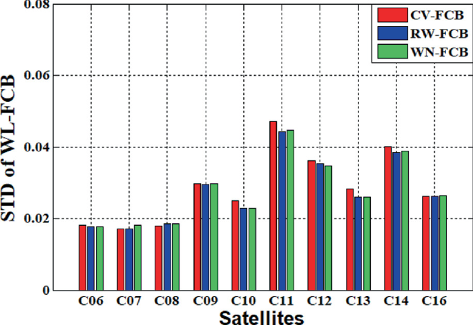
STD of undifferenced wide-lane FCB


The distribution of FCB posterior residuals is an index that can directly reflect the accuracy of FCB products. The posterior residuals of wide-lane FCB with annual product date of the 6th day of 2019 are selected. As shown in Fig. 4, it can be seen that the posterior residuals distribution of satellite FCB of three BDS are basically the same. Table 1 is the residual distribution of three wide-lane FCB in 7 days. It can be seen from the table that the estimation accuracy of FCB of three wide lanes is basically the same, indicating that It shows that different ISB processing strategies have no effect on wide-lane FCB estimation accuracy.

Posterior residuals of three wide-lane FCBs
-
2)
Analysis on undifferenced narrow-lane FCB characteristics
The ionosphere-free ambiguity is affected by narrow-lane FCB, so high precision of narrow-lane FCB is the key to PPP-AR. Compared with wide-lane FCB, the stability of narrow-lane FCB is low. The FCB of narrow-lane with 10 min interval is estimated as random walk process, and once is estimated every 10 min. The single day time-varying characteristics of three kinds of narrow-lane FCB are shown in Fig. 5. (a) is IGSO satellite narrow-lane FCB, and (b) is MEO satellite narrow-lane FCB. And it can be seen that the FCB stability of IGSO satellite is better than that of MEO satellite.

Three narrow-lane FCB series of BDS satellites
In order to further analyze the accuracy of different FCB products, Posterior residuals of the narrow-lane FCB product on the 6th day of 2019 is selected, and the distribution is shown in Fig. 6. It can be seen that the residual distribution of RW-FCB and WN-FCB in narrow-lane is similar, and it is obviously better than CV-FCB in narrow-lane, which increases about 10% in (−0.25, +0.25) cycle, 14% in (−0.15, +0.15) cycle, and 18% in (−0.05, 0.05) cycle. In Table 2, the residual distribution of three kinds of narrow-lane FCB in 7 days is counted. It can be seen from the table that compared with CV-FCB, RW-FCB and WN-FCB about improvement 7.5%, 10.6% and 12.2% in (−0.25, +0.25), (−0.15, +0.15) and (−0.05, +0.05), respectively, which indicates that different ISB processing strategies have great influence on FCB estimation accuracy of narrow-lane, and ISB should be regarded as random walk process or white noise estimation. The possible reason is that narrow-lane ambiguity is more sensitive to the error, and the inappropriate parameter processing strategy has a greater impact on the narrow-lane ambiguity, so the precision of narrow-lane FCB is relatively lower.

Posterior residuals of three narrow-lane FCB
4.2 Positioning Result Analysis
Table 3 Statistics the time to first fix and fixed rate of ambiguity of 13 stations using three FCB products. It can be seen from the table that PPPAR-RW and PPPAR-WN are better than PPPAR-CV model in average time to first fix and fixed success rate of ambiguity, with an increase of about 19.5% and 15.5%, respectively. Table 4 shows the positioning accuracy of 13 stations using three FCB products. The 3D positioning accuracy of PPPAR-CV model is 11.07 cm, 7.35 cm and 6.09 cm in 30 min, 60 min and 120 min, respectively. PPPAR-WN and PPPAR-RW are basically the same, but better than PPPAR-CV, which are improved by about 6.3 cm, 3.9 cm and 3.6 cm respectively. It can be seen that the inaccurate processing of ISB parameters has a great influence on the narrow-lane ambiguity which is more sensitive to the error, which influence the convergence accuracy of short-time ambiguity, reduces the estimation accuracy of FCB in narrow-lane, and further affects the time to first time, fixed rate and short-time fixed solution accuracy of ambiguity (Table 4).
5 Conclusions
In this paper, through different ISB processing strategies, using the 106 evenly distributed IGS/MGEX station network, are used to estimate three FCBs product, namely CV-FCB, RW-FCB and WN-FCB. The effects of different ISB processing strategies on FCBs estimation accuracy and PPP-AR positioning are analyzed:
-
1)
When ISB is treated as constant, white noise and random walk process, the accuracy of FCB products in wide-lane FCB is equivalent. In narrow-lane FCB, the accuracy of WN-FCB and RW-FCB is the same, which is better than CV-FCB products. In the range of (−0.25, +0.25), (−0.15, +0.15), (−0.05, +0.05) cycle, the accuracy of WN-FCB and RW-FCB are increased by 7.5%, 10.6% and 12.2%, respectively.
-
2)
In terms of the first convergence time and fixed success rate of ambiguity, PPPAR-WN and PPPAR-RW are basically the same, which are improved by about PPPAR-CV model, they are improved by about 19.5% and 15.5% respectively.
-
3)
in terms of positioning accuracy, the 3D positioning accuracy of PPPAR-CV model is 11.07 cm, 7.35 cm and 6.09 cm at 30 min, 60 min and 120 min respectively, while PPPARRW and PPPAR-WN are basically equivalent, but better than PPPAR-CV, with an increase of about 6.3 cm, 3.9 cm, 3.6 cm at 30 min, 60 min, 120 min.
References
Yuanxi, Y.: Progress, contribution and challenges of compass/beidou satellite navigation system. Acta Geodaetica Cartogr. Sin. 39(1), 1–6 (2010)
Yangyin, X., Yuanxi, Y., Haibo, H., Jinlong, L., et al.: Quality analysis of the range measurement signals of test satellites in BeiDou global system. Geomat. Inf. Sci. Wuhan Univ. 43(8), 1214–1221 (2018)
Yang, Y.X., Li, J.L., Wang, A.B., et al.: Preliminary assessment of the navigation and positioning performance of BeiDou regional navigation satellite system. Sci. China Earth Sci. 57(1), 144–152 (2014)
Thoelery, S., Steigenberger, P., Montenbruck, O., et al.: Signal analysis of the first GPS III satellite. GPS Solutions 23, 92 (2019)
Jokinen, A., Feng, S., Milner, C., et al.: Improving fixed-ambiguity Precise Point Positioning (PPP) convergence time and accuracy by using GLONASS. In: International Technical Meeting of the Satellite Division of the Institute of Navigation. 2012, pp. 3708–3727 (2012)
Li, P., Zhang, X.: Integrating GPS and GLONASS to accelerate convergence and initialization times of precise point positioning. GPS Solutions 18(3), 461–471 (2014)
Jokinen, A., Feng, S., Schuster, W., et al.: GLONASS aided gps ambiguity fixed precise point positioning. J. Navigation 66(3), 399–416 (2013)
Tegedor, J., Øvstedal, O, Vigen, E.: Precise orbit determination and point positioning using GPS, Glonass, Galileo and BeiDou. J. Geodetic Sci. 4(1), 2081–9943 (2014)
Research on Methodology of Rapid Ambiguity Resolution for GNSS Precise Point Positioning. Wu Han: Wuhan University (2016)
Zhou, Z.: Theory and Methods of Precise Point Positioning and Its Quality Control with Multi-GNSS. Information Engineering University (2018)
Li, X., Ge, M., Dai, X., et al.: Accuracy and reliability of multi-GNSS real-time precise positioning: GPS, GLONASS, BeiDou, and Galileo. J. Geodesy 89(6), 607–635 (2015)
Cai, C., Gao, Y., Pan, L., et al.: Precise point positioning with quad-constellations: GPS, BeiDou, GLONASS and Galileo. Adv. Space Res. 56(1), 133–143 (2015)
Lou, Y., Zheng, F., Gu, S., et al.: Multi-GNSS precise point positioning with raw single-frequency and dual-frequency measurement models. GPS Solutions 20(4), 849–862 (2016)
Chen, J., Zhang, Y., Wang, J., et al.: A simplified and unified model of multi-GNSS precise point positioning. Adv. Space Res. 55(1), 125–134 (2015)
El-Mowafy, A., Deo, M., Rizos, C.: On biases in precise point positioning with multi-constellation and multi-frequency GNSS data. Measurement ence Technol. 27(3), (2016)
Jin, W., Yuanxi, Y., Qin, Z., et al.: Analysis of inter-system bias in multi-GNSS precise point positioning. Geomatics Inf. Sci. Wuhan Univ. 44(004), 475–481 (2019)
Liu, T., Yuan, Y., Zhang, B., et al.: Multi-GNSS precise point positioning (MGPPP) using raw observations. J. Geodesy 91(3), 253–268 (2017)
De Bakker, P.F., Tiberius, C.C.J.M.: Real-time multi-GNSS single-frequency precise point positioning. GPS Solutions 21(4), 1791–1803 (2017)
Feng, Z., Danan, D., Pan, L., et al.: Influence of stochastic modeling for inter-system biases on multi-GNSS undifferenced and uncombined precise point positioning. GPS Solutions 23(3), 59–71 (2019)
Xiaohong, Z., Pan, L., Xingxing, L., Feng, Z., Xiang, Z.: An analysis of time-varying property of widelane carrier phase ambiguity fractional bias. Acta Geodaetica Cartogr. Sin. 42(6), 798–803 (2013)
Author information
Authors and Affiliations
Editor information
Editors and Affiliations
Rights and permissions
Copyright information
© 2021 The Author(s), under exclusive license to Springer Nature Singapore Pte Ltd.
About this paper

Cite this paper
Qi, W., Chai, H., Kun, X., Min, W., Yang, C. (2021). Influence of Different ISB Processing Strategies on the Accuracy of Undifferenced FCBs and PPP-AR Positioning. In: Yang, C., Xie, J. (eds) China Satellite Navigation Conference (CSNC 2021) Proceedings. Lecture Notes in Electrical Engineering, vol 773. Springer, Singapore. https://doi.org/10.1007/978-981-16-3142-9_23
Download citation
DOI: https://doi.org/10.1007/978-981-16-3142-9_23
Published:
Publisher Name: Springer, Singapore
Print ISBN: 978-981-16-3141-2
Online ISBN: 978-981-16-3142-9
eBook Packages: EngineeringEngineering (R0)