Research and Application of Horizontal Well Cross-Layer Fracturing Technology in Tight Sandstone Reservoir

Abstract

At present, in horizontal well fracturing of tight sandstone reservoirs, artificial fractures can not cross through the mudstone barrier layer vertically and fracturing fluid can pass through mudstone barrier layer, but proppant cannot, which make effective placement of proppant only in sandstone layer at horizontal well section, and reduce the fracturing effect. This paper studied the influencing factors of fracture propagation and extension in tight sandstone reservoirs by laboratory experiments, reservoir evaluation, simulation calculation and field tests. Through comprehensive optimization of fracturing technology, such as fracturing fluid viscosity, construction fluid volume, injection displacement, proppant type and injection mode, artificial fractures can be fractured through mudstone barrier layer and proppant can be effectively propped up in fractures. The results show that the main influencing factors of fracture propagation and extension in tight sandstone reservoir are fracturing fluid viscosity, construction displacement and fluid volume in turn. On this basis, the construction technology was optimized so that artificial fracture can penetrate all thin interbeds of sandstone and mudstone vertically, without causing uncontrolled fracture height, and improving the effective placement of proppant in fractures. The research results were carried out in thin interbedded sandstone reservoirs in Jianghan Basin. The results show that fracturing by this technology can effectively cross through thin interbedded sandstone and mudstone, improve the effective placement of proppant in fractures, and increase the effective reconstruction volume. The stimulation effect was better than the conventional horizontal well fracturing method for the same type of reservoirs, the production was higher and the stable production period was longer. This paper improved the fracturing effect of this kind of reservoir.

1 Introduction

In recent years, horizontal well fracturing technology has been widely used in the development of tight sandstone thin interbedded reservoirs. Different from single-thin layer fracturing, thin interbedded layer fracturing belongs to multi-layer fracturing, which involves longitudinal penetration of vertical fracture. The main technical limitations of thin interbedded layer fracturing in horizontal wells are as follows: inaccurate stress state of vertical sand and mudstone, unclear law of fracture height expansion, even the situation that all sand and mudstone layers are not communicated vertically. The use of conventional particle size and density proppant, and the single particle size type is in the majority, which results in most proppants providing fracture conductivity in the sandstone where the horizontal wellbore is located [1, 2]. Therefore, in order to achieve vertical cross-layer fracturing, artificial fractures need to pierce mudstone barriers between multiple sand layers, and proppants need to be transported into target sandstone layers above and below horizontal wellbore and effectively laid. Based on the establishment of crustal stress model, this paper studied the influencing factors of vertical extension of fracturing fracture in tight sandstone, and through comprehensive optimization of fracturing fluid, construction fluid volume, injection displacement and proppant etc., horizontal well cross-layer fracturing was realized, which enlarged effective reconstruction volume and improved fracturing effect.

2 Rock Mechanics and Crustal Stress Model

Rock mechanics parameters are one of the basic data for reservoir stimulation. They reflect the physical and mechanical properties of rock from deformation to fracture under various external forces, such as hardness, brittleness index, compressive strength, shear strength and so on. There are two main methods for calculating rock mechanics parameters [3]: one is field measurement, which simulates the underground environment (temperature, confining pressure, pore pressure) of rock in laboratory by using the core obtained from drilling. The other is the calculation method, which uses geophysical logging data for inversion calculation. The latter method has the characteristics of large depth of analysis, continuous data, economy and high efficiency because of its relatively easier acquisition of logging data. Taking the tight sandstone reservoir of Jianghan Oilfield as an example, the reservoir in this area belongs to the typical tight sandstone thin interbedded layer reservoir. The static and dynamic data such as rock mechanics experiment, logging and fracturing data are synthesized to interpret rock mechanics and crustal stress parameters in order to restore the real stress profile as far as possible.

2.1 Rock Mechanics Model

• (1) Construction of shear wave transit time curve

  The correlation fitting of P-S wave obtained by orthogonal dipole acoustic logging was carried out. Because the P-S wave relation curves of sandstone and mudstone are quite different [4], the shale content (SH) was used to fit the P-S wave relation curves by weighting and introducing the SH curve. A more reliable P-S wave relation was obtained, as shown in Figs. 1 and 2.

  Fig. 1.

  

  S-P wave relation fitting based on logging data

  Fig. 2.

  

  S-P wave relation fitting combined with argillaceous content

  Combining the above analysis, we could get the suitable S-P wave transit time fitting relation for this block as follows.

  $$ t_{s} = 1.1479\Delta t_{p} - \frac{53.99}{GR} $$

  (1)

• (2) Correction of Dynamic and Static Rock Mechanics Parameters

  There are two commonly used methods for measuring rock mechanical parameters: dynamic method and static method. Static method is obtained by static loading of rock sample and dynamic method is obtained by measuring the propagation velocity of ultrasonic wave in rock. The Young’s modulus and Poisson’s ratio of a single well interpreted by the calculation model of the corresponding relationship between logging and rock mechanics were compared with the experimental results, and the corresponding relationship between dynamic and static Young’s modulus and Poisson’s ratio could be fitted. Poisson’s ratio, Young’s modulus and other parameters were closely related to shale content [5]. Therefore, SH curve was introduced to improve fitting accuracy, as shown in Figs. 3 and 4.

  Fig. 3.

  

  Dynamic and static relation fitting of Poisson’s Ratio

  Fig. 4.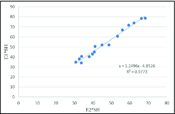

  

  Dynamic and static relation fitting of Young’s Modulus

  Combining with the above analysis, the static Poisson’s ratio and Young’s modulus formulas suitable for this block could be obtained as follows.

  $$ \mu = 0.7844\mu_{D} + \frac{1.379}{SH} $$

  (2)
  $$ E = 1.2496E_{D} - \frac{4.8526}{SH} $$

  (3)

  In the formula: $\mu$ - static Poisson’s ratio, $E$ - static Young’s modulus, MPa.

2.2 Crustal Stress Model

The formula for calculating the self-weight of overlying strata and the induced horizontal stress was as follows.

$$ S_{v} = \int_{0}^{h} {\rho (h) \cdot g \cdot dh} $$

(4)

$$ S_{x1} = S_{y1} = \frac{\mu }{1 - \mu } \cdot (S_{v} - \alpha \cdot P_{p} ) + \alpha \cdot P_{p} $$

(5)

In the formula: $S_{v}$ - vertical principal stress, MPa. $\rho (h)$ - rock bulk density, kg/m³. $g$ - gravity acceleration, m/s². $S_{x1}$, $S_{y1}$ - horizontal crustal stress, MPa. $\mu$ - formation rock Poisson’s ratio. $P_{p}$ - formation pore pressure, MPa.

The formula for calculating tectonic stress was as follows.

$$ S_{x2} = \xi_{x} \cdot (S_{v} - \alpha \cdot P_{p} ) + \alpha \cdot P_{p} $$

(6)

$$ S_{y2} = \xi_{y} \cdot (S_{v} - \alpha \cdot P_{p} ) + \alpha \cdot P_{p} $$

(7)

In the formula, $\xi_{x}$, $\xi_{y}$ - the tectonic stress coefficients in horizontal X and Y directions respectively; $S_{x2}$, $S_{y2}$ - the tectonic stress caused by tectonic movement in horizontal X and Y directions respectively, MPa.

The formula for calculating the total crustal stress was as follows.

$$ S_{H} = S_{x1} + S_{x2} $$

(8)

$$ S_{h} = S_{y1} + S_{y2} $$

(9)

In the formula: $S_{H}$ - maximum horizontal principal stress, MPa; $S_{h}$ - minimum horizontal principal stress, MPa.

The formula for calculating the effective crustal stress was as follows.

$$ \sigma_{H} = S_{H} - \alpha \cdot P_{p} $$

(10)

$$ \sigma_{h} = S_{h} - \alpha \cdot P_{p} $$

(11)

In the formula: $\sigma_{H}$ - maximum horizontal effective stress, MPa; $\sigma_{h}$ - minimum horizontal effective stress, MPa.

According to the above calculation model, the crustal stress of some wells in this block were calculated, as shown in Table 1.

Table 1. Statistics of crustal stress profile interpretation results of some wells in Jianghan Oilfield

3 Analysis of Main Controlling Factors of Fracture Height Extension

In the process of hydraulic fracturing, there are many factors affecting the extension of hydraulic fracture height, which can be divided into two main categories [6]: geological factors and engineering factors. Geological factors mainly include elastic modulus, Poisson’s ratio, formation permeability, fracture brevity, interface effect and formation heterogeneity. Engineering factors mainly include construction displacement, construction fluid volume, fracturing fluid viscosity, fracturing fluid filtration coefficient, fracturing fluid gravity coefficient, etc. [7]. Geological factors are uncontrollable factors and engineering factors are controllable factors. In this paper, the main engineering factors such as construction displacement, construction fluid volume and fracturing fluid viscosity were studied and analyzed.

Taking the average construction parameters of the block as the initial value, the influence law of each factor was analyzed by GOHFER software orthogonal simulation calculation. The model parameter settings were shown in Table 2.

Table 2. Parameter setting of main controlling factor analysis model for fracture height extension

3.1 Fracturing Fluid Viscosity

From Figs. 5 and 6, it could be seen that the higher the viscosity of fracturing fluid was, the higher the artificial fracture extended, and the easier it was to pierce the barrier. When fracture fluid viscosity increased from 50 mPa.s to 200 mPa.s, fracture height increased from 19 m to 43 m. Fracture fluid viscosity had a great influence on fracture height extension. The use of medium and low viscosity fracturing fluid (<100 mPa.s) could effectively control fracture height extension and increase fracture length. When the fracturing fluid viscosity was larger than 100 mPa.s, the artificial fracture was easy to break through the barrier.

Fig. 5.

Effect of fracturing fluid viscosity on fracture extension

Fig. 6.

Fracture extension under different fracturing fluid viscosities

3.2 Construction Displacement

From Fig. 7, it could be seen that the higher the construction displacement was, the higher the artificial fracture extended, and the easier it was to pierce the barrier. When the injection displacement was more than 4 m³/min, the fracture pierced the barrier. The more the liquid entered the fracture in a short time, the greater the net pressure in the fracture was and the faster the fracture longitudinally extended. In the process of thin layer fracturing, if high displacement construction was used all the time, it would lead to excessive extension of fracture height in the early stage of fracturing, which would affect effective fracture length, and low displacement construction could effectively control the extension of fracture height. Variable displacement construction could take into account the requirements of controlling fracture height, piercing barrier and adding sand with high sand ratio.

Fig. 7.

Effect of construction displacement on fracture extension

3.3 Construction Fluid Volume

From Fig. 8, it could be seen that the larger the amount of construction fluid was, the higher the artificial fracture extended, and the easier it was to pierce the barrier. Because when the amount of construction fluid increased, the amount of liquid used to increase the volume of fracture was larger, and the length and height of fracture would increase accordingly. Moreover, under the same construction displacement, the lower formation permeability was, the more obvious the influence of construction scale on fracture height was.

Fig. 8.

Effect of construction fluid volume on fracture extension

Through the above analysis, we quantified the influence of various engineering factors on the fracture height extension. From Table 3, we could see that the influencing factors of fracture height extension from large to small were as follows: fracturing fluid viscosity, construction discharge and fluid volume. The higher the viscosity of fracturing fluid was, the higher the artificial fracture extended, and the easier it was to pierce the barrier. The use of variable viscosity fracturing fluid could give consideration to both the height of fracturing and making fracture. The larger the displacement of fracturing construction was, the higher the artificial fracture extended, and the easier it was to pierce the barrier. The variable displacement construction could take into account both sand adding and fracture height controlling. The larger the amount of fracturing fluid was, the higher the artificial fracture extended, and the easier it was to pierce the barrier.

Table 3. Change rate of fracture height with doubling of influencing factors

Table 4. Fracturing data

4 Fracturing Technology Optimization

This block was a typical tight sandstone reservoir. The reservoir mainly consisted of thin/multi-thin layers. The reservoir thickness mainly concentrated on 2 m–10 m. The average porosity of main layers was 7.3% by logging interpretation, and the average permeability was 0.46 mD. It belonged to low porosity and ultra-low permeability reservoir. The average thickness of the barrier in this area was 3.2 m, and the average stress difference of the barrier was 4.9 MPa. According to the reservoir conditions in this area, the fracturing technology was optimized.

4.1 Optimization of Fracturing Fluid Viscosity, Construction Displacement and Proppant

In order to pass through mudstone shield layer and migrate into sandstone target layers above and below horizontal wellbore, and evenly distribute and effectively lay artificial fractures longitudinally, ultra-low density proppant was selected. Considering the requirements of different stages of fracturing, 70/140 mesh, 40/70 mesh and 30/50 mesh proppant were selected. Considering the sand carrying capacity of fracturing fluids with different viscosities, small size proppants (70/140 mesh) were carried with low viscosity fracturing fluid (15 mPa. s), medium size proppants (40/70 mesh) were carried with medium viscosity fracturing fluid (50 mPa. s), and large size proppants (30/50 mesh) were carried with medium and high viscosity fracturing fluid (100 mPa. s). The influence of fracturing fluid viscosity and construction displacement on fracture extension was analyzed by comprehensive simulation. From Fig. 9, it could be seen that the higher the fracturing fluid viscosity was, the greater the sensitivity of fracture height to displacement was, and the easier the artificial fracture to penetrate the barrier was. When the displacement was larger than 4 m³/min, the longitudinal fracture extension accelerated and the artificial fracture penetrated the barrier.

Fig. 9.

Fracture extension law under different displacement and fracturing fluid viscosity

4.2 Optimization of Construction Fluid Volume and Proportion of Pre-fluids

According to the comprehensive simulation analysis of the influence of construction fluid volume and proportion of pre-fluid on the longitudinal extension of fracture, when using low-viscous fracturing fluid, the construction fluid volume reached 700 m³ to pierce the barrier. When using medium-viscous fracturing fluid, the construction fluid volume reached 600 m³ to pierce the barrier. When using high-viscous fracturing fluid, the construction fluid volume reached 400 m³ to pierce the barrier. From Fig. 10, it could be seen that the lower the proportion of pre-liquid was, the easier the fracture to pierce the barrier was at the same liquid volume (Fig. 11).

Fig. 10.

Relationship between fracture fluid viscosity, construction fluid volume and fracture height

Fig. 11.

Relation between pre-liquid ratio, construction fluid volume and fracture height

5 Application Example

Well A was in a thin-bedded block of Jianghan Basin. The lithology of the target layer was brown-gray oil-tracked siltstone, and natural fractures were well developed. The fracturing layers of the target formation were 2570.8–2574.0 m and 2575.5–2577.2 m. The average Young’s modulus of the reservoir was 27.2 GPa and the average Poisson’s ratio was 0.23. The stress difference between the target layer and the upper layer was about 4.5 MPa, and the stress difference between the target layer and the lower layer was about 8.5 MPa, and the temperature of the target layer was 105 ℃. By using the fracturing technology in this paper, artificial fractures pierced the mudstone barrier between sand layers. Through the optimization of proppant and injection mode, proppant was smoothly transported into the target sandstone layers above and below the horizontal wellbore through the narrow fracture width of mudstone and effectively laid, thus effectively solving the problem of vertical fracture penetrating layers and realizing vertical fracturing through layers.

5.1 Optimization of Fracturing Fluid System

According to the development characteristics of tight and low permeability and fracturing technology, it was required to select fracturing fluid system with good properties such as low residue, low breaking glue viscosity and low surface tension. Considering all aspects, we adopt clean fracturing fluid system. On the one hand, through adjusting the fluid viscosity at different stages of fracturing, we could maximize the demand of cross-layer fracturing, improving conductivity and sand-carrying requirements in the main sand-adding stage, on the other hand, we could minimize the damage to reservoirs. Three sets of clean fracturing fluid systems with low viscosity, medium viscosity and high viscosity were selected. The low viscosity was 10 mP.s to 15 mP.s, the medium viscosity was 40 mP.s to 50 mP.s, and the high viscosity was 110 mP.s to 130 mP.s.

5.2 Optimization of Construction Parameter

Combining logging data, experimental data and GOFHER software simulation analysis results, 260 m³ low viscosity fracturing fluid was injected in the pre-fluid stage with a low displacement of 2.0–3.0 m³/min, 241 m³ medium viscosity fracturing fluid and 346 m³ high viscosity fracturing fluid were injected in the sand-carrying stage with a medium-high displacement of 3.5–6.0 m³/min.

5.3 Optimization of Proppant

Multi-stage proppant slug with 70/140 mesh was injected in the early sand-carrying stage, which was divided into three stages, the sand-liquid ratio was 3%, 6%, 9% and the stage sand volume was 15.3 m³. Ultra-low density proppant with 40/70 mesh was selected in the middle stage, and low sand ratio of 6% was used in the initial stage, then the sand ratio was gradually increased to the maximum of 18% with 3% increment, and the stage sand volume was 16.5 m³. The ultra-low density proppant with 30/50 mesh was selected in the later stage. In the initial stage, medium sand ratio of 10% was used, and then the sand ratio was gradually increased to the maximum of 30% with 5% increment, and the sand volume was 20.8 m³ in the stage.

According to the above steps, the fracturing construction of this well was carried out successfully (Table 4). Combining with the well temperature logging interpretation results and the secondary simulation results of fracture after fracturing (Table 5 and Fig. 12), it was confirmed that the fracture longitudinally cross through the lower mudstone shield layer, and the sandstone in the horizontal section was effectively laid with proppant. The well had achieved good stimulation effect. The initial oil production was 8.5 m³/d, and it was stable about 6.0 m³/d after half a year. The effect was better than that of similar wells in this area.

Table 5. Interpretation results of fracturing fracture parameters

Fig. 12.

Fracture simulation nephogram

6 Conclusion

• (1) Because the P-S wave relationship, Poisson’s ratio, Young’s modulus and other parameters of sandstone were closely related to shale content, shale content was introduced to modify and fit these parameters. Rock mechanics and crustal stress parameters could be accurately calculated by using the revised data.

• (2) The engineering factors affecting fracture hight extension in tight sandstone reservoirs were fracturing fluid viscosity, construction displacement and fluid volume in turn.

• (3) Horizontal well cross-layer fracturing technology suitable for tight sandstone thin layer reservoir was formed, which enabled artificial fracture to pierce mudstone barrier between multiple sand layers, proppant could cross through mudstone barrier layer into the target layer of sandstone above and below the horizontal wellbore and lay it effectively, solving the problem of vertical fracture cross-layer and expanding the effective stimulation volume.

References

Kang, Y., Luo, P.: Current status and prospect of key techniques for exploration and production of tight sandstone gas reservoirs in China. Pet. Explor. Dev. 34(2), 239–244 (2007)
Su, Y., Mu, L., Fan, W., et al.: Optimization of fracturing parameters for ultra-low permeability reservoirs. Pet. Drill. Tech. 39(6), 69–72 (2011)
Xie, F., Chen, Q.: Observations and researches of crustal stress. Int. Earthq. Dyn. 29(2), 1–7 (1999)
Wang, G., Shao, W., Wang, L., et al.: A method study on identifying light oil and gas reservoir using compressional/shear speed ratio based on the variable matrix interval transit time. Well Logging Technol. 32(3), 246–248 (2008)
Yao, C., et al.: Determination of Yong’s modulus by using conventional logging – take upper paleozoic reservoirs of Fuxian block as an example. Pet. Geol. Eng. 26(5), 110–112 (2012)
Lai, B.: Experimental study on fracturing limit of thin interbedded layers. Inner Mongolia Petrochem. Ind. 38(24), 150–151 (2012)
Zhou, W., et al.: Current status and researching points of technology of artificially controlling fracture height. Nat. Gas Explor. Dev. 29(1), 68–70 (2006)
Author information
Authors and Affiliations
Corresponding author
Editor information
Editors and Affiliations
Rights and permissions
Copyright information
© 2020 Springer Nature Singapore Pte Ltd.
About this paper
Cite this paper
Wu, Zy., Hu, Yf., Jiang, Tx., Liu, Jk., Wu, Cf. (2020). Research and Application of Horizontal Well Cross-Layer Fracturing Technology in Tight Sandstone Reservoir. In: Lin, J. (eds) Proceedings of the International Field Exploration and Development Conference 2019. IFEDC 2019. Springer Series in Geomechanics and Geoengineering. Springer, Singapore. https://doi.org/10.1007/978-981-15-2485-1_41
Download citation
DOI: https://doi.org/10.1007/978-981-15-2485-1_41
Published:
Publisher Name: Springer, Singapore
Print ISBN: 978-981-15-2484-4
Online ISBN: 978-981-15-2485-1
eBook Packages: EngineeringEngineering (R0)