Composite Property Testing, Characterization, and Quality Control

Abstract

Property testing, characterization, and quality control are three major issues in advanced composite research, development, and applications. These also are common concerns for material scientists, structural designers, and users of composite materials.

Editors for this chapter: Zuoguang Zhang, Zilong Zhang.

Property testing, characterization, and quality control are three major issues in advanced composite research, development, and applications. These also are common concerns for material scientists, structural designers, and users of composite materials. To extend the application of advanced composites, especially in high-tech areas, the performance stability of composites should be characterized to justify the use of composites in a design. To fulfill these requirements, advanced composite testing, characterization, and quality control are required.

Composites are multiple material systems composed of two or more different materials fabricated with the use of physical and chemical processing techniques. Composites must be considered in terms of their various constituents, combinations of materials, and their structural processing and multilayer construction. Each of these factors presents difficulties for achieving high standards for composite property testing, characterization, and quality control.

In terms of materials and processing, the stability of a given property is an important factor, which affects advanced composite quality. Factors that can influence composite stability are summarized as follows:

• ① Lack of knowledge about materials characteristics: For many features of composites, there are currently no perfect theories available to explain and predict their properties. In many cases, empirical approaches are the main tool for evaluating composite performance. Owing to the lack of a systemic understanding of composite features, it is very difficult to accurately evaluate the stability of composite properties.

• ② Variation of constituent properties: The non-uniformity of constituent materials results in a certain scatter of their performance. The performances of composites not only depend on their constituent materials, but also the combination of constituents.

• ③ Instability of processing techniques: Knowledge is limited on the physical and chemical mechanisms currently used to prepare composite materials. This results in poor reproducibility of processing and a large scatter in the performance of materials.

• ④ Imperfectness of testing methods: As a relatively new kind of material, currently there are no suitable methods and standards to test and inspect certain properties of composites. In the established standards, specimens cannot perfectly reflect the real-world performance of composite structures. There is much work required on evaluating composite stability by nondestructive testing.

• ⑤ Lack of statistical data: Compared with traditional materials, data on composite performances are severely limited. In many databases, typical values are given with insufficient statistical data.

• ⑥ Lack of knowledge about the regularity of changes in composite material properties over time: Composite matrices are very sensitive to time- and temperature-dependent effects and their performances will change with time. Current accumulated data still does not reflect the behavior of composites over a full range of ambient conditions and different time periods.

This chapter is divided into six sections focusing on issues surrounding testing of composite properties, characterization, and quality control. In Sects. 5.1 and 5.2, methods for testing composite properties, developing test plans, processing test data, and matrix testing, are discussed. In Sect. 5.3, prepreg performance characterization and characterization technologies, physical parameters, and processing ability characterization are introduced. In Sect. 5.4, laminate property testing is discussed, including test methods for basic physical and mechanical properties, fracture toughness, and damage resistance. In Sect. 5.5, composite quality evaluation and control are examined together with a discussion on the complexity of quality evaluation and existing problems. Two quality evaluation approaches are first proposed to address the quality control of composites. Three processing quality control methods are also introduced. The final section concerns composite failure analysis.

5.1 Guidelines for Composite Property Testing

Composite property testing is of great importance in composite design selection, processing quality control, product quality inspection, assembly, and repairs. The properties of composites have implications for the overall course of material development, structure design, processing, manufacture, quality evaluation, and service and maintenance. Much attention has been paid to these aspects and many test methods and related techniques have been developed. Some of these methods have now become standards, and most are based on test methods for traditional metal materials. However, compared with traditional metallic materials, composites have several unique features to consider such as small rates of extension, anisotropic properties, internal structure complexity, and sensitivity to applied load. These features can cause problems for traditional test methods, including: ① Currently, most test methods only give apparent test results rather than the intrinsic characteristics. ② Testing results depend strongly on the specimen dimensions with a large size effect. This makes it difficult to evaluate the equivalence between specimens of different sizes. ③ There are many methods available for testing the same material property, which makes it difficult to select more suitable and reliable methods. ④ Test results are often not compatible with the practical effectiveness. ⑤ Many methods are complex, time-consuming, and difficult to implement. Thus, the development of more rigorous and effective test methods requires the establishment of more reasonable test systems and standardization of test data from composite materials.

5.1.1 Features of Property Characterization of Composites

Property characterization is an important topic in materials research and structural applications. For polymer matrix composites, the property characterization has special importance as outlined below:

• (1) Unlike isotropic metals, composites are composed of two or more constituents. Thus, the characterization should start by examining the constituents.

• (2) The failure mechanisms are different from those of traditional metals and test methods developed for metals are not suitable for composites. Hence, the development of new test methods is needed.

• (3) Owing to some unique features, many new requirements have been proposed for composite property characterization, in particular the hot–wet characteristics and impact resistance.

• (4) Composites are highly designable. The structural laminates are composed of plies with different fiber ratios and orientations, which contribute to the characteristic complexities of laminates—the basic structure element.

• (5) Composite materials and their structure are simultaneously determined during manufacture. Thus, variations of materials and processing will affect the material and structure.

• (6) Owing to a lack of experience with composite materials, structure design, and applications, the building block approach is an important approach for verification of composites (Fig. 5.1). Property characterizations may be divided into five levels: constituent, lamina, laminate, structural element, assembled component, and higher levels. Thus, more levels are involved for composites materials than for metals in terms of the categories and numbers of samples.

  Fig. 5.1

  

  Building block approach for composite verification

• (7) Property characterization is important for structure development based on composite materials. On the basis of the application of the data, the characterization testing can be divided into the following types: material screening, material verification, material acceptance, material equivalent evaluation, and structural certification.

Owing to the importance of property characterization in the development and production of composites characterization and the standardization are important aspects in the field of composite materials. Standardization encompasses two key aspects: the scope and method of property characterization (including test standards, sample quantity, and data processing), and the recommended test matrices for different applications.

As applications of composite materials have been extended, methods for their standardization have also progressed. For example, the MIL-HDBK-17 (Handbook of Composites) and ASTM D30 composite division are being continuously revised and updated.

5.1.2 Test Design and Classification

Test activities can be defined into two basic approaches, the structural complexity level and the data application category. The classes within each are discussed in more detail in the following sections and can be used to set out large-scale testing programs to guide test planning.

• (1) Structure complexity levels

The five structural complexity levels¹ are each based on geometry or form: constituent, lamina, laminate, structural element, and structural subcomponents. The five structural complexity levels cover the following areas:

• (1) Constituent testing: This evaluates the individual properties of fibers, fiber forms, matrix materials, and fiber-matrix preforms. Key properties, for example, include fiber and matrix density, fiber tensile strength and tensile modulus, and fracture elongation.

• (2) Lamina testing: This level evaluates the properties of the fiber and matrix together in the composite material. For the purposes of this discussion prepreg properties are included in this level, although they are sometimes broken down into a separate level. Key properties include fiber area weight, matrix content, void content, cured ply thickness, lamina tensile strengths and moduli, lamina compressive strengths and moduli, and lamina shear strengths and moduli.

• (3) Laminate testing: Laminate testing characterizes the response of the composite material in a particular laminate design. Key properties include tensile strengths and moduli, compressive strengths and moduli, shear strengths and moduli, interlaminar fracture toughness, and fatigue resistance.

• (4) Structure element testing: At this level, the ability of a material to tolerate common laminate discontinuities is evaluated. Key properties include open- and filled-hole tensile strengths, open- and filled-hole compressive strengths, compression after impact strength, and joint bearing and bearing bypass strengths.

• (5) Structural subcomponent (or higher level) testing: This testing level evaluates the behavior and failure modes of more complex structural assemblies, which are usually used in verification tests based on lower-level testing.

The material form(s) to be tested, and the relative emphasis placed on each level, should be determined early in the material data development planning process. The selection of test forms will likely depend upon many factors, including: the manufacturing process, structural application, corporate/organizational practices, and the procurement and/or certification agency. While a single level may suffice in rare instances, most applications will require at least two levels, and it is common to use all five in the complete implementation of the building block approach. Regardless of the selected structural complexity level, physical or chemical characterization of the prepreg properties (or matrix, if it is included as part of the process, as for resin transfer molding) is necessary to support the physical and mechanical property test results. Each procurement or certification agency has specific minimum requirements and guidelines for use of data. It is advisable to coordinate with the procuring or certifying agency before planning to ensure testing is conducted, which supports these structural qualification or certification.

• (2) Data application categories

Other than classifications based on structural complexity, material property testing can also be grouped in terms of the data application into one or more of the following five categories: screening,² qualification, acceptance, equivalence, and structural substantiation. The starting point for testing most material systems is usually material screening. Material systems intended for use in engineering hardware are subjected to further testing to obtain additional data. The five data application categories cover the following areas:

• (1) Screening testing: This is the assessment of material candidates for a given application, often with a particular application in mind. The purpose of screening testing is initial evaluation of new material systems under worst-case environmental and loading test conditions. This handbook provides guidelines for screening new material systems based on key properties for aerospace structural applications. The MIL-HDBK-17 screening test matrix provides average values for various strength, moduli, and physical properties, including both lamina and laminate level testing, and is designed both to eliminate deficient material systems.

• (2) Material qualification testing: This step proves the ability of a given material/process to meet the requirements of a material specification. This step is also the process for establishing the original specification requirement values. Rigorous material qualification testing considers the statistics of the data and is ideally a subset of, or directly related to the design allowable testing, performed to satisfy structural substantiation requirements. However, while a material may be qualified to a given specification, it must still be approved for use in each specific application. The objective is quantitative assessment of the variability of key material properties, leading to statistical data that are used to establish material acceptance, equivalence, quality control, and design basis values. Because there are various sampling and statistical approaches used within the industry, the approach used must be explicitly defined. A generic basis value can be obtained in many ways: Each user’s basis value carries with it well-defined sampling requirements and a specific statistical determination process. There is also an emphasis on additional considerations such as test methodology, failure modes, and data documentation.

• (3) Acceptance testing: This is the task of verifying a material’s consistency through periodic sampling of the product and evaluation of key material properties. Test results from small sample sizes are statistically compared with control values established from prior testing to determine whether or not the material production process has changed significantly.

• (4) Equivalence testing: This task assesses the equivalence of an alternate material to a previously characterized material, often for the purpose of using an existing material property database. The objective is to evaluate key properties of test populations large enough to provide a definitive conclusion, but small enough to avoid the costs of generating an entirely new database. A common application includes evaluation of potential secondary sources for a previously qualified material, and for evaluation of minor changes to constituents, constituent processing, or fabrication processing from a qualified material system. The testing aims to substantiate the replacement material based on previously established basis values.

• (5) Structural substantiation testing: This is the process of assessing the ability of a given structure to meet the requirements of a specific application. The development of design allowables is considered a part of this step. The allowables should ideally be derived or related to material basis values obtained during materials qualification.

A matrix is shown in Table 5.1, which illustrates a common testing sequence in the substantiation of a composite-based aerospace structural application. The material property tests from the structural complexity levels and data application categories are listed on the axes of an array, with each intersecting cell describing a distinct testing activity. Groups of cells can be used to summarize the scope of unique test programs. The sequence begins with the hatched cells at the upper left of the array and proceeds, with time, toward the cells at the lower right, with the numbered notes indicating the approximate order of the test sequence.

Table 5.1 Test program definition

5.1.3 Test Program Planning

All major testing programs should begin with the preparation of a detailed test plan document. Characterization of composite material properties is distinctly different for that of metals and unreinforced plastics. There are many critical factors that affect testing and test planning. In addition to the material properties to be tested, the method of testing and the preparation of the specimens should be specified in the testing program. Other factors such as the testing acceptance and requirements for nondestructive evaluation, data processing, and specimen moisture absorption, which can affect the test results, should be considered in the testing program. A full discussion of these issues will be the focus of this section. In addition, consideration will be given to material operation limits and property testing under ambient and non-ambient conditions, because of their importance in testing of composite structural properties.

5.1.3.1 Test Property Selection

Composites are produced from two or more different materials. The multiple raw materials and complexity of the composition, including anisotropic properties and “dimensional effects” in hot–wet conditions, mean that it is uneconomical to evaluate and test all properties. In practice, only those properties that are critical to the composite application will be selected and evaluated. The main factors will be the critical test method and test conditions. Special applications may involve some other factors.

In lamina level tests, the material strength and stiffness are selected including the tensile, compression and shear strength, and moduli. Measurements of the 0° tensile and compression in the longitudinal direction can provide the static strength and stiffness. The ±45° tensile strength is used to determine the shear modulus and the effective strength. Laminate testing also aims to test features of discontinuous stress, such as fastener element holes, bolt by-passing bearing, and impact damage. These tests are usually performed at room temperature. The effects of environment can be evaluated by lamina tensile and open-hole compression testing. Finally, the compression after impact (CAI) is used to evaluate the damage resistance.

For composite materials to be used at high temperature or in special liquid environments, further high-temperature resistance and liquid sensitivity tests should be performed. High-temperature performance typically involves dry-wet high-temperature static mechanical tests, thermal-oxidation stability, and thermal cycle fatigue tests. The highest exposure temperature for thermal-oxidation stability and thermal cycle fatigue tests should be selected between the wet and dry glass transition temperatures. The thermal oxidative stability (TOS) test should be performed for a minimum of 1000 h. Weight loss should be measured during testing at specified intervals of 100, 250, 500, 750, and 1000 h. This test is a measure of the oxidation rate of a material. Thermal cycle fatigue tests should be performed for a minimum of 500 thermal cycles at a specified temperature. Over the course of the test, crack generation and crack growth rates should be determined to characterize the thermal fatigue resistance of the composite.

The liquid sensitivity test is mainly used to evaluate the possibility of property changes caused by long-term contact with chemical agents, such as fuel oil, hydraulic fluid, detergent, and ice removing agents. For example, epoxy resin exposed to strongly acidic media can undergo degradation and high-temperature BMI and polyimide resins are easily degraded by strong alkali conditions. Liquid sensitivity tests can be also used to evaluate the resistance of the composite to liquids, which are likely to come into contact with the part. In some cases, additional modifiers may change the resin resistance to solvents. For example, polysulfone thermoplastic composite structures have lower resistance to hydraulic fluid; however, some other thermoplastic materials give good resistance to moisture and hydraulic fluid, but poor fuel oil resistance.

5.1.3.2 Test Method Selection

Although the basic physics of test methods for composite materials are similar to those for testing metals or plastics, the heterogeneity, orthotropic, moisture sensitivity, and low ductility of typical composites often lead to major differences in test requirements, particularly for mechanical tests. These differences include:

• (1) The strong influence of constituent content on material response necessitates measurements of the material response of every specimen.

• (2) Properties should be evaluated in multiple directions.

• (3) Specimens should be conditioned to quantify and control moisture absorption and adsorption.

• (4) The methods of specimen alignment and load induction have increased importance for composites.

• (5) The consistency of failure modes requires some assumptions to be made.

Thus, many historical test methods which have been developed for metals or plastics cannot be directly applied to advanced composite materials in most cases. Other distinguishing characteristics of many composite materials also contribute to differences in testing. For example, compressive strength is often lower than tensile strength, operating temperatures are closer to the material’s transition temperatures, the shear stress response is uncoupled from the normal stress response, and specimens are highly sensitive to the preparation methods.

Therefore, to properly evaluate the properties of composites, suitable testing methods should be developed. Many investigations on different test methods have been performed and standards have been established. However, current testing methods remain inadequate.

One measure of a test method is the ability of a perfect test to reproduce a desired behavior, such as the uniform uniaxial stress state. However, the above factors tend to increase the sensitivity of composites to a wider variety of testing parameters than those affecting traditional materials. Therefore, the robustness of a test method, or its relative insensitivity to minor variations in the specimen and test procedure, is just as important as theoretical perfection. Robustness, or lack thereof, is assessed by interlaboratory testing, and is measured by precision (variation in the sample population) and bias (variation of the sample mean from the true mean).³ The precision and bias of test methods are evaluated by comparison testing (often called “round-robin” testing) both within-the same and between external laboratories. An ideal method should have high precision (low variation) and low bias (sample mean close to true average) both within-laboratory and between laboratories. Such a test method would repeatedly give reproducible results regardless of the material, operator, or test laboratory. However, quantification of bias requires a material standard for each test. Such standards are not currently available for composites. As a result, bias of composite test methods can currently only be qualitatively assessed.

Other separate issues from the precision and bias of a test method (for a given specimen) are the effects of test specimen size and geometry on precision and bias. For heterogeneous materials, physically larger specimens can be expected to contain a more representative sample of the material microstructure. Although this is desirable, a larger specimen is more likely to contain more micro- or macro-structural defects than a smaller specimen and can be expected to produce somewhat lower strengths. Variations in specimen geometry can also create differing results. Size and geometry effects can produce statistical differences in results independent of the “degree of perfection” of the remaining aspects of a test method. Therefore, an “ideal” test method will use a specimen geometry that can be consistently correlated with its structural response.

The criticality of various test parameters is not yet well understood and the subject of current research. Furthermore standard practices, may vary from laboratory to laboratory upon close examination. Hence, methods should be selected that are commonly used, easily controlled, and meet the user’s requirements. For example, mechanical testing using a unidirectional specimen will generally not enable effective or reproducible results. Therefore, alternate approaches are often used. For example, [90/0]_ns cross-ply laminates are often used for static mechanical testing, and the equivalent unidirectional strength and stiffness can be calculated based on laminate theory. Cross-ply laminates have been shown to have a large tolerance to secondary deviations in specimen preparation and testing implementation, which can often give high average strength measurements and low scatter of data. In terms of practical applications, it is commonly thought that cross-ply laminates are more representative of the material response of structural laminates.

In addition, the testing methods and parameters used should be detailed in specifications to reduce the variation caused by some occasional factors.

5.1.3.3 Population Sampling

In material property testing, results may be different from each other even if the materials, testing methods and conditions are maintained, and the data may show considerable scatter. In general, the properties of composites will change between different batches. Furthermore, data should not be acquired from a single testing condition. Instead, a testing population should be used based on many factors such as temperature, moisture, and ply layer sequence. To obtain results with high reliability, data from enough specimens are needed to ensure that the testing results are sufficiently reproducible to meet engineering accuracy requirements. The level of data deemed to be sufficient depends on many factors including: statistical models for population sampling, the necessary replicates of a desired result (i.e., the selection of A-basis and B-basis values), the deviation of the measured properties from those under practical conditions, and the deviation of the measured properties caused by testing methods.

Owing to the reasons mentioned above, the sample size cannot be strictly defined; instead, only general guidelines can be given according to the application requirements. According to the statistical model applied, a larger sample number will be needed for a Weibull distribution model than that required for a normal distribution model. The A-basis value is a 95% lower confidence bound of the first percentile of a specified population of measurements, while the B-basis is a 95% lower confidence bound on the tenth percentile of a specified population of measurements. Thus, the A-basis requires much more data than B-basis for a given replicate.

Population sample sizes include the selection of sample size of each batch and the selection of batch numbers. For general data development, sampling techniques and sample sizes will depend on the application or qualification/certification agency. Any sampling scheme should have multiple batches composed of uniformly sized subpopulations. These two aspects will be discussed in the following:

• (1) Sample size selection

Regardless of the sampling scheme, for small sample populations, the results of any basis value calculation depend strongly on the sample size. Smaller sample populations are clearly less costly to test; however, as the population size decreases, so does the value of the calculated basis. Figure 5.2 shows, a hypothetical example, the effect of sample size on the calculated B-basis value for samples of various sizes drawn from a given infinite normally distributed population. In the limit, for very large sample sizes, the B-basis (tenth percentile) value for this example would be 87.2. The dotted line in the figure is the mean of all possible B-basis values for each sample size; this line can also be interpreted as the estimated B-basis value as a function of population size for a fixed sample coefficient of variation (CV) of 10%. The dashed lines represent the 1−σ limits for any given sample size (a 2−σ limit would approximately bound the 95% confidence interval).

Fig. 5.2

Normalized B-basis of 1−σ limits

It can be seen from this figure, not only does the estimated B-basis value increase with larger sample sizes, but, as the 1−σ limits illustrate, the expected variation in the estimated B-basis value significantly decreases. The lower 1−σ limit is farther from the mean B-basis value than the upper 1−σ limits, illustrating a skewing of the calculated B-basis value, which is particularly strong for small sample sizes. As a result of this skew, for small populations the calculated B-basis value is much more likely to be over-conservative than under-conservative. This result increases the penalty paid for B-basis values determined from the use of small populations. While similar examples for non-normal distributions show different quantitative results, the trends with sample size can be expected to be similar.

• (2) Batch quantity selection

If the data variation between samples is caused by occasional factors in the same batch, the property data between different batches will show a much more complex deviation. For example, many factors such as raw materials, processing history, and the state of equipment can cause large variations of properties between batches. If testing is performed only on samples from a single batch, and the average result approaches a constant value, this constant will be different from that obtained from testing of different batches. The former reflects convergence to a certain value of a specific population batch, while the latter is the real convergence to the total population average value (full average value). The differences of the average values between the total population and a special single population are the second variance of the measured material property values. This variation is a random measurement and will change from batch to batch. Therefore, statistical approaches should be used to determine the variation between batches, and the batch quantity should be determined according to the needs of a specific property test.

If the resulting statistical analysis indicates excessive batch-to-batch variation, the data are not conventionally pooled but should instead be evaluated using Analysis of Variance (ANOVA). It is often necessary to add batches to generate more statistical data. When the statistical analysis shows no clear variation between batches compared with that within a single batch, the data obtained from different batches can be merged and a smaller number of batches can be used to perform testing.

Small numbers of batches can cause ANOVA to produce extremely conservative basis values, because it essentially treats the average of each batch as a single data point for input into a conventional normal distribution technique for basis value determination. This statistical method assumes that the test variation is negligible, and that variation caused by testing, either within or between batches, is treated as real material/process variation, which can result in unrealistically low basis values. Also, the between-batch variation test becomes progressively weaker as the number of batches decreases or as the variation between batches decreases, or both. For example, when only a small number of batches are sampled, a batch variation test result that indicates no significant batch variation may be not be reliable. Testing of additional batch samples may indicate that the batch variation exists, but was masked by the original small number of batches. Attention should be paid to this issue when batch variation exists and the ANOVA basis values are calculated based on less than five batches.

5.1.3.4 Material and Processing Variation

The majority of fibers, resins, and composite material forms and structural elements are the products of complex multistep materials processes. Figure 5.3 illustrates the nature of processing from raw materials to a finished composite product. These processes may involve elevated temperatures, stress, and pressure. The procedures often involve evolution of volatiles, resin flow and consolidation, and readjustment of the reinforcing fibers. As shown in Fig. 5.4, each rectangle represents a process during which additional variability may be introduced into the material. In Fig. 5.3, each obtained product will become the raw material for the next processing step. The variations of materials and processing in this processing are often superimposed. If the measured properties of composite materials are to be interpreted correctly and used appropriately, the variability of the properties of the materials must be understood. This variability arises during routine processing and may be increased by the various anomalies that may occur during processing.

Fig. 5.3

Basic flow chart of composite processing

Fig. 5.4

Raw material flow chart of composite processing

Currently, polymer matrix composites are most widely used. These composites feature organic matrices (either thermosetting or thermoplastic) and organic or inorganic reinforcing fibers. Variation of the mechanical properties of the reinforcing fibers can arise from many sources, such as flaws in the fiber microstructure, or variation in the degree of orientation of the polymer chains in the organic fibers. Damage can also be induced during filament merging and product delivery; hence, a layer of protective coating is usually applied to the fiber surface.

Thermoplastic matrices can exhibit variations in the molecular weight and molecular weight distribution of the polymer as a result of processing. The melt viscosity and resulting processability of a thermoplastic matrix can be strongly affected by such variability. Thermosetting resins are often applied to fibers in a prepregging operation and in some forms, are partially cured to a so-called B-stage. Other methods for stabilizing thermosetting resin systems may also be used before the prepregging operation. Stability of these materials is important because there are many potential sources of variability during packaging, shipping and storage of improperly, and even properly, stabilized intermediate forms such as prepreg tape, fabrics, and roving.

Compared with handling of raw materials, property variation is more often encountered during the composite processing step. For example, the placement of reinforcing fibers or prepreg tapes may be accomplished through manual or automated processes with high precision. Lack of precision in fiber placement or subsequent shifting of the reinforcing fibers during the matrix flow and consolidation can introduce variability. Depending on the curing process, consolidation can occur simultaneously with the fiber placement, or after the fiber placement. This step in the process is especially vulnerable to the introduction of variability. For example, consider the curing of a composite part from a B-staged prepreg tape in an autoclave, a press, or an integrally heated tool. When the resin is heated and has begun to flow, the material consists of a gas phase (volatiles or trapped air), a liquid phase (resin), and a solid (reinforcement) phase. To avoid variability in material properties due to excessive void volume, the void producing gas phase material must be either removed or absorbed by the liquid phase. To avoid variability caused by variations in the fiber volume fraction, the resin must be uniformly distributed throughout the part. The fiber must maintain its selected orientation to avoid variability or loss of properties due to fiber misalignment.

In general, during the selection of raw materials and processing implementation, pertinent processing parameters and material effects should always be documented to support process control and troubleshooting. If potential processing and manufacturing pitfalls are not identified and avoided in this way, resources may be wasted in testing materials, which are not representative of those that occur in the actual part or application. Furthermore, heavy weight penalties might be paid to allow for avoidable material variability. A better understanding of these processing parameters and their potential effects on material properties will also allow a composites supplier or manufacturer to avoid the considerable expenses involved in the production of materials, parts, or end items, which have unacceptable properties.

5.1.3.5 Sample Preparation and Inspection

• (1) Sample preparation

The validity of material properties used in design of a structure depends on the quality of the tested specimens. If the objective of the testing is to provide comparative information of different materials, it is crucial that variability due to specimen preparation be minimized. If the data being generated are intended for the generation of an allowable, the aim should be to reflect the interaction of the base material and processing, which may be expected to occur in production. In either case, care must be taken in the specimen preparation process to minimize the variation, which naturally occurs during the process. Issues to consider in specimen fabrication include specimen traceability, test article⁴ fabrication, specimen location, configuration, and machining.

• (1) Traceability: all specimens should be traceable to the material batch number, lot number, and roll number. Each specimen should be traceable to its location within the test article and processing information, should be included in the specification to enable full traceability. When uncured materials are purchased all available traceability information, including vendor certifications, and material inspection data of acceptance test results, should be delivered with the material. All prepreg materials that are stored before fabrication should have a storage history record. Information such as accumulated time in and out of refrigeration should be recorded.

• (2) Test article fabrication: the following is a list of important items that should be considered when fabricating test articles:

  • ① Test articles should be built according to engineering drawing requirements or sketches. The drawing requirements or sketches should specify: ply materials, test article reference orientation, ply orientation, material and process specifications or equivalent process documents, and inspection requirements.

  • ② Important material and process identification, such as prepreg batch number, lot number, roll number, autoclave run, pressing or other consolidation method, and layer stacking sequence should be recorded. This information should be stored to maintain the traceability of the test articles. This same traceability should be maintained for any excess material left after the specimens have been removed.

  • ③ The test article identification code and witness line should be permanently identified on each test article. A witness line should be established on the fabrication tool to act as a reference to the fiber orientation of the test article. For hand-laying methods, a witness line should be maintained during the layup and curing process and identified as a reference for the orientation.

    The angular tolerance between the plies depends on the processing specifications applied to the material. For automated processes, some other method of establishing the reference orientation must be established. Once established, the witness line should be transferred to the test article and maintained throughout the specimen extraction.

  • ④ It is generally recommended that for cured test articles at least 1 in. (25 mm) of material be trimmed from the edges. One of the machined edges of the test article may be used to permanently maintain the reference orientation on the article.

  • ⑤ The requesting organization (or if required, the appropriate quality assurance organization) should inspect test articles. This inspection should be performed before the specimens are fabricated to ensure that all requirements are met in the control process specification or appropriate equivalent document.

• (3) Specimen fabrication: The following is a list of important points that should be considered when fabricating specimens.

  • ① Specimens should be extracted from test articles in the region that meets all process, engineering drawing, and specimen drawing requirements.

  • ② Specimens should be located on the test article according to the cutting diagram provided by the requesting organization. If a test article does not pass the inspection criteria, the requesting organization may choose to cut specimens relative to the identified test article defects to ensure that effects of the defects on the specimen response are representative of the full-scale item.

  • ③ A specimen identification code should be defined in the test plan, referenced in the test instructions, and recorded in the data sheets. The specimen identification code should be permanently marked on each specimen. Care should be taken to mark the code outside the failure area of the specimen.

  • ④ For specimens too small to allow marking with the complete code, a unique serial number may be marked on the specimen. It is recommended that care is taken to place small specimens in bags properly labeled with full identifying information.

  • ⑤ If it is required that the location of the specimen on the test article be known, specimens should be labeled before being extracted. This labeling method should allow all specimen and excess material locations to be known after cutting.

  • ⑥ The reference edge of the specimen should be aligned with the specified orientation by the witness line. In instances where a smaller subtest article is machined and used to make several specimens at once, a reference line or edge should be transferred to the subtest articles from the witness line. This transfer line should be orientated within ±0.25° with respect to the witness line.

  • ⑦ Specimens should be extracted from the fabricated test articles according to the appropriate machining procedure as specified. Specimens may be machined with a variety of machining tools. In general, the final cutting tool should have a fine grit, be hardened, and run at a high tool speed without wobble. The cut itself should be executed to minimize excess heating of the laminate.

  • ⑧ The added cost and manufacturing associated with tabbed specimens should be considered when selecting specimen type. The limitations and problems associated with tabbing of specimens are stated in each individual test method. If bonded tabs are required, the cure of the adhesive should be evaluated to determine if it is compatible with the composite system and tab material (if different). If the tab configuration produced in the bonding process is not within the geometry requirements of the specimen configuration, further machining of the tabs may be required.

  • ⑨ Holes in specimens should be drilled in accordance with the applicable process specifications.

  • ⑩ Any fasteners that are required should be installed in accordance with the applicable process specifications.

Completed specimens should be inspected prior to testing to ensure conformance with the standards being used. Variation in individual specimen thickness should be within the applicable test method tolerances. Larger variations may cause improper loading when used with close tolerance test fixtures. These variations may indicate that the specimen was fabricated improperly (e.g., ply drop-off or resin bleeding).

• (2) Nondestructive evaluation

In specimen preparation, composites will be subject to mechanical machining, which may cause damage to specimens. To acquire correct test results, a nondestructive examination (NDE) report should be submitted together with the specimens by the manufacturer. If necessary, the test operator should conduct a nondestructive testing (NDT) inspection when accepting a specimen to verify the inspection report submitted by the manufacturer. If a specimen contains defects from the preparation, such defects should be verified and the location and dimensions indicated by the user.

Commonly used NDT inspection methods include visible inspection, tapping, supersonic inspection, and acoustic emission and infrared thermal imaging. In general, no single method can be applied to all types of defect/damage in a composite structure, and two or more methods may be required for real applications.

5.1.3.6 Moisture Absorption and Conditioning Factors

Most polymeric materials, whether in the form of a composite matrix or a polymeric fiber, are capable of absorbing relatively small amounts of moisture from the surrounding environment.⁵ This absorbed water may produce dimensional changes (swelling), lower the glass transition temperature of the polymer, and reduce the matrix and matrix/fiber interface dependent mechanical properties of the composite, effectively lowering the maximum use temperature of the material. Because absorbed moisture is a potential design concern for many applications, material testing should include evaluations of properties after representative moisture exposure.

• (1) Description of moisture absorption

Assuming there are no cracks or other wicking paths, the physical mechanism for moisture gain is generally assumed to be mass diffusion following Fick’s law.

While material surfaces in direct contact with the environment absorb or desorb moisture almost immediately, moisture flow into or out of the interior occurs relatively slowly. The moisture diffusion rate is many orders of magnitude slower than heat flow in thermal diffusion. Nevertheless, after a few weeks or months of exposure to a humid environment, a considerable amount of water will eventually be absorbed by the material. The amount of moisture absorbed by a material depends on its thickness and the exposure time. The moisture properties of a material can be expressed by two parameters: moisture diffusivity and moisture equilibrium content (weight percent moisture). These properties are commonly determined by gravimetric testing methods.

The rate of moisture absorption is controlled by a material property, moisture diffusivity. Moisture diffusivity is usually only weakly related to relative humidity and is often assumed to be a function only of temperature, following an Arrhenius-type exponential relation with an inverse absolute temperature. This strong temperature dependence is illustrated in Fig. 5.5, which shows moisture diffusivity versus temperature for a particular type of carbon/toughened epoxy.

Fig. 5.5

Moisture diffusivity as a function of temperature

Moisture equilibrium content is only weakly related to temperature and is usually assumed to be a function only of relative humidity. The largest value of moisture equilibrium content for a given material under humid conditions occurs at 100% relative humidity and is also often called the saturation content. The moisture equilibrium content at a given relative humidity has been found to be approximately equal to the relative humidity multiplied by the material saturation content; however, as illustrated by Fig. 5.6, this linear approximation does not necessarily hold well for all material systems. Regardless, if a material does not reach the moisture equilibrium content for a given relative humidity, then the local moisture content will not be uniform through the specimen thickness. Furthermore, moisture absorption properties under atmospheric humid conditions are generally not equivalent to liquid immersion or exposure to pressurized steam. These latter environments alter the material diffusion characteristics, producing higher moisture equilibrium content, and should not be used unless they simulate the relevant application environment.

Fig. 5.6

Equilibrium moisture content versus relative humidity

• (2) Sample immersion process

There are two methods for sample immersion treatment: One is fixed-time immersion, in which the sample is exposed to a moisture environment for a specified time period. Another method is equilibrium immersion, in which the sample exposure is terminated when the equilibrium between the sample and moisture environment is reached. Although fixed-time immersion is still commonly used in materials screening, this approach results in non-uniformity of the moisture absorption along the sample thickness direction. Thus, fixed-time immersion is not sufficiently representative and is only used for some screening-level purposes or as part of a structure application-level testing program. Instead, a conditioning procedure should be followed that accounts for the diffusion process and terminates with a nearly uniform moisture content through the thickness.

When absorbed moisture is included in the design, the evaluation of material moisture absorption characteristics (diffusion rate and equilibrium content) should be included in the material testing program. The effects of moisture on some key design properties after environmental exposure should also be considered.

• (1) Fixed-time immersion: As stated earlier, fixed-time conditioning has only limited usefulness and cannot generally provide the desired uniform moisture conditions through the thickness of the material. The shortcomings of the fixed-time approach are illustrated in Fig. 5.7 for a simulated 30-day exposure of IM6/3501-6 carbon/epoxy at 60 °C and 95% relative humidity (RH). With the use of known values for moisture diffusivity and moisture equilibrium content, the calculated average moisture content of various laminate thicknesses can be plotted as a smooth curve. From this curve, the maximum laminate thickness that can reach equilibrium at this temperature during this fixed conditioning exposure is 0.89 mm. For greater thicknesses, the moisture distribution through the thickness will not be uniform, as the interior moisture levels will be below the equilibrium moisture content.

  Fig. 5.7

  

  Two-sided moisture absorption of carbon/epoxy laminate after 30 days exposure at 60 °C/95% RH

  As seen from the examples above, total moisture content resulting from fixed-time conditioning is thickness dependent. However, because fluids diffuse through different materials at different rates, fixed-time conditioning cannot produce uniform conditions for all materials,⁶ even if the thickness is constant. Therefore, test results based on fixed-time conditioning should not be used for design values, and generally should not even be used in qualitative comparisons between different materials.

• (2) Equilibrium immersion: To evaluate worst-case effects of moisture content on material properties, tests are performed with specimens preconditioned to the design service (end-of-life) moisture content. The preferred conditioning methodology should include procedures for the conditioning, as well as the determination of moisture diffusivity and moisture equilibrium content.

  ASTM D5229/D5229 M is a gravimetric test method that exposes a specimen to a moisture environment and plots moisture mass gain versus the square root of elapsed time, as shown in Fig. 5.8. The early portion of the mass/square root time relationship is linear, the slope of which is related to the moisture diffusivity. As the moisture content of the material near the surface begins to approach equilibrium, the gradient of this curve becomes increasingly small. Eventually, as the interior of the material approaches equilibrium, the difference between subsequent weighing steps will be very small and the slope will be nearly zero. At this point, the material is said to be at equilibrium moisture content. This process is illustrated in Fig. 5.8, where the different curves show the difference in response at different temperatures. At 66 °C condition (diamonds in Fig. 5.8), the moisture profile through the thickness of the specimen, as shown in Fig. 5.9, illustrates the rapid moisture uptake near the surface at soon after exposure and the relatively slow uptake of moisture in the middle of the specimen.

  Fig. 5.8

  

  Typical moisture absorption response

  Fig. 5.9

  

  Through thickness moisture profile versus time

• (3) Accelerated immersion conditioning: Because equilibrium moisture conditioning can take a very long time, it is desirable to accelerate the process. Certain two-step, accelerated conditioning cycles are considered acceptable, such as use of an initial high-humidity step (95% RH) to speed up moisture gain, followed by a stage at a lower final humidity level (85% RH) before equilibrium is reached. However, the selection of an accelerating environment should not change the material or alter the physics of diffusion. Because the moisture diffusion rate is so strongly dependent on temperature, it is tempting to accelerate the process by increasing the conditioning temperature. However, long-term exposure to high temperatures and moisture may alter the chemistry of the material. Cure epoxy-based materials are typically not conditioned above 82 °C to avoid these problems; materials that cure at lower temperatures may need to be conditioned below 82 °C. While an initial high relative humidity step is acceptable, extreme cases of exposure to pressurized steam or immersion in hot/boiling water are not accepted methods of accelerating humidity absorption, as these methods have been found to produce different results from those measured at 100% humidity.⁷

• (4) General procedures for immersion: The procedural descriptions and requirements are fairly complete for some standards; however, the following points should be emphasized:

  • ① It is highly recommended that before performing conditioning some knowledge of the material moisture response be obtained, either from the literature or from prior testing.

  • ② In moisture property measurements the actual specimen must be initially dry, and the precision and timing of early mass measurements is critical. For the purposes of material conditioning, knowledge of the initial moisture content may not be important, or may be separately determined from other specimens in parallel. Therefore, moisture conditioning is not normally performed with a material dry out step. Moisture conditioning also does not require repetitive, precise weighing early in the exposure process that is necessary to determine the moisture diffusivity. Thus, conditioning without simultaneous determination of the moisture absorption properties is faster and less labor intensive.

  • ③ If the moisture properties are desired, it is faster and less labor intensive to create two other sets of specialized moisture property specimens, including a thin set that will reach equilibrium quickly, and a thick set, from which a stable slope to the moisture weight gain versus square root time curve can be reliably obtained with minimum test sensitivity.

Moisture content measurements should be performed by either weighing the actual specimens, or by weighing “travelers,” in their place. The travelers are material conditioned specimens cut from the same panel and conditioned at the same time as the specimens. Travelers are required when the specimen is either too small, too large, or includes other materials, such as specimens with tabs or sandwich specimens. A traveler accompanies the specimen or group of related specimens, throughout the conditioning process. Because the weight gain of typical polymeric composites is relatively small (on the order of 1%), mass measurement equipment must be selected accordingly. For larger specimens (>50 g), a balance accurate to 0.001 g is generally adequate. For smaller specimens with a mass of the order of 5 g, a precision analytical balance capable of reading to 0.0001 g is required. Direct moisture mass monitoring of coupons weighing less than 5 g is not recommended; a traveler should be used instead.

Near the end of conditioning, minor weighing errors or small relative humidity excursions of the environmental chamber, particularly slight depressions in the relative humidity, may artificially cause the material to appear to have reached equilibrium, when, in fact, the material is still absorbing moisture. At lower temperature (lower diffusion rates), these errors become more important. In view of the possibility of these experimental errors, a prudent engineer should consider the following measures.

• ① Even after the material appears to satisfied the definition of equilibrium, review the chamber records to ensure that a depression in chamber relative humidity did not occur during the reference time period (weighing time interval). If such a depression is found to have occurred, continue the exposure until the chamber has stabilized, then processed to point ②.

• ② Even after the material satisfies the definition of equilibrium, maintain the exposure, and ensure satisfaction of the criteria for several consecutive reference time periods.

If a drying step is included, either as an initial step prior to moisture conditioning, or as part of an oven-drying experiment, care should be taken to avoid excessively high drying temperatures and high thermal excursions that may induce thermal cracking of the material.

For a specific material and relative humidity, a variant of equilibrium conditioning uses equilibrium conditioning test data to establish a relationship between the minimum exposure times required to achieve equilibrium versus laminate thickness. This approach eliminates many repetitive weighing steps.

• (3) Conditioning and test environment

In immersion processes, the required equilibrium RH depends on the practical application. The designed service moisture content is only a semi-empirical calculated value, and for aircraft structural composites, this value is between 80% and 85% RH based on different calculations. Thus, 85% RH is used as the test condition for equilibrium moisture content, if no other particular need is specified.

Hot–wet testing should use specimens conditioned to equilibrium moisture content and tested at the material operational limit (MOL) temperature or below. The effects of environment are generally small for matrix-dependent properties at temperatures below room temperature. Owing to these factors, qualification/certification testing programs typically do not require moisture conditioning below room temperature. Because there is generally no need to determine a cold MOL, specimens are simply tested at the coldest design service temperature (often −55 °C).

5.1.3.7 Non-ambient Testing Environments

Composite materials can be affected by exposure to non-laboratory ambient environmental conditions and must be tested to determine those effects. Temperatures above and below ambient laboratory temperatures must be included in the test matrix to determine the effects of these environments. Many different regimes of testing may be appropriate depending on the usage of the materials. Normal environmental conditions for terrestrial applications can range from temperatures of −55 °C up to 180 °C. Conditions in space widen the range of performance temperatures from −160 °C to 230 °C. Cryogenic conditions less than −160 °C may also be of interest for storage tank applications. Special conditions may dictate the use of composite materials up to and beyond 315 °C around leading edges or engine components. Composites used in space applications will also be subjected to ultraviolet radiation, atomic oxygen, micrometeoroid debris, and a charged particle environment. Thus, it is necessary to specify the application of materials to identify the required non-ambient test environmental conditions. The following discussion will examine high- and low-temperature testing conditions.

• (1) Subambient testing

Testing performed below laboratory ambient test temperatures should use special fixtures or lubrication to ensure that the properties measured are related to material behavior and not due to freezing or sticking of sliding surfaces. Further challenges will be encountered in most cases. Materials can become more brittle and change their failure modes. Special instrumentation may be necessary to record material properties at cold temperatures. Adhesives used for tabbing or strain gaging should retain their elongation properties at cold temperatures.

Test temperatures as cold as −55 °C are common and considered to be representative. The cooling medium may be liquid nitrogen (LN₂), liquid carbon dioxide (LCO₂), or a refrigerated chamber. Temperature measurements are commonly made with J, K or T type thermocouples (T/C). The test setup in a test chamber must be precooled until stabilization at the test temperature. A dummy test specimen should be used to determine the soak times prior to actual testing. The dummy specimen should be fabricated from the same material and with the same ply orientation as those of the test specimen. To determine the soak time, a T/C should be inserted into a hole drilled at the centerline of the dummy specimen. The time taken to reach the desired test temperature should be recorded and this time should be used when testing to ensure the test specimens are at the appropriate test temperature. Cool down rates should be controlled to minimize thermal shock and the possibility of damage and/or microcracking.

Freezing of test fixtures can cause anomalous test results. Fixture clearances must be checked to ensure free sliding surfaces. Proper lubrication or no lubricants should be used at the cold temperatures to prevent any fixture related effects on the test results. A thermocouple (T/C) should be placed in contact with the surface of the test specimen at the time of test. A typical soak time of 5–10 min, or the time determined from actual experimentation, should be used, after reaching the test temperature. Appropriate safety equipment should always be worn to prevent cold burns. Care must be taken if using liquid N₂ or dry ice (CO₂) when cooling the chamber to ensure that room oxygen is not depleted.

• (2) Above ambient testing

Testing above ambient temperatures must be performed with consideration for the temperature and moisture content of the test sample. Special fixtures may be needed to accommodate the high temperatures. The possibility of adhesive failure and drying of test specimens should be evaluated before proceeding with a test program. Special lubricants may be required to prevent fixtures from sticking or binding. Instrumentation made especially for the required temperatures must be used to ensure valid data is recorded. Strain gauges, extensometers, and adhesives with the correct temperature rating must be identified and used. Special strain gauge foils or backing materials may be required to withstand elevated temperatures during testing. Instrumentation may require additional calibration at the test temperatures.

Above ambient test temperatures can typically reach temperatures as high as 180 °C. As for the case of subambient testing, the test setup in a test chamber must be heated until stabilization at the test temperature. Fixtures should be allowed to stabilize prior to testing. Heating of the test fixture with specimens, or the specimen only, is usually accomplished with an electrically heated chamber. To determine the soak time, a T/C should be inserted into a hole drilled at the centerline of the dummy specimen. The time taken to reach the desired test temperature should be recorded. This time should be used when testing to regulate the appropriate test temperature for the specimens. Heat up rates should be controlled to minimize thermal shock and the possibility of damage and/or microcracking. Excessive heat up rates may cause charring or melting of test specimens or adhesives. An appropriate lubricant, such as molybdenum disulfide, should be used on sliding surfaces to ensure freedom of movement of test fixtures.

For moderate test conditions, i.e., less than 93 °C, a humidity controlled test chamber is optional for short duration tests. When testing above 93 °C, then precise humidity control is impractical and specimen dry out is a concern, especially for fatigue testing. A standard soak time is 5–10 min, after reaching the test temperature, if the test conditions are dry. If the test conditions are wet, soak times prior to the test should be kept short (<3 min) to minimize dry out.

Testing performed at temperatures above 180 °C must use special strain gauges and strain gauge adhesives, extensometers, and fixtures designed for the elevated temperatures. Special high-temperature-capable tab materials and tab adhesives are needed to prevent tab failures.

5.1.4 Data Reduction

5.1.4.1 Data Outlier Screening and Processing

An outlier is a data point that is much lower or much higher than the majority of other observations in a data set. Outliers are often erroneous values, perhaps caused by clerical errors, incorrect setting of environmental conditions during testing, or a defective test specimen. Data should routinely be screened for outliers, because these values can have a substantial influence on the statistical analysis. The maximum normed residual (MNR) method is used for quantitative screening for outliers.

• (1) The maximum normed residual

The MNR test is a screening procedure for identifying an outlier in an unstructured set of data. A value is declared to be an outlier by this method if it has an absolute deviation from the sample mean which, when compared to the sample standard deviation, is too large to occur by chance. The MNR method can only detect one outlier at a time; hence, the significance level pertains to a single decision.

Let x ₁, x ₂,…, x _n denote the data values in a sample of size n, and let $\overline{x}$ and s be the sample mean and sample deviation, respectively. The MNR statistic is the maximum absolute deviation from the sample mean divided by the sample standard deviation:

$$ {\text{MNR}} = \frac{{\hbox{max} \left| {x_{i} - \overline{x} } \right|}}{s}(i = 1,2,\varLambda ,n) $$

(5.1)

The MNR value is compared with the critical value for the sample size n from Eq. (5.1). If the MNR is smaller than the critical value, then no outliers are detected in the sample; otherwise, the data value associated with the largest value of $\left| {x_{\text{i}} - \overline{x} } \right|$ is declared to be an outlier.

$$ C = \frac{n - 1}{\sqrt n }\sqrt {\frac{{t^{2} }}{{n - 2 + t^{2} }}} $$

(5.2)

where t is the [1 − α/(2n)] quantile of the t-distribution with n–2 degrees of freedom and α is the significance level. The recommended significance level for this test is α = 0.05.

If an outlier is detected, this value is omitted from the calculations and the MNR procedure is applied again. This process is repeated until no outliers are detected. Note that the jth time that a sample is screened for an outlier, the mean, standard deviation, and critical value are computed based on a sample size of n − j − 1. It should be noted that for small samples, for example a batch containing five or six data, this procedure may identify most of the data as outliers, particularly if two or more of the values are identical. In this case, observational methods can be used to identify outliers.

• (2) Disposition of outlier data

When outlier data are detected, the first action should be to identify evidence of a physical cause. The following list gives some examples of conditions that could be used as the basis for discarding outlier data.

• (1) The material (or a constituent) was out of specifications.

• (2) One or more panel or specimen fabrication parameters were outside the specified tolerance range.

• (3) The test specimen dimensions or orientation were outside the specified tolerance range.

• (4) A defect (not under study) was present in the test specimen.

• (5) An error was made in the specimen preconditioning (or conditioning parameters were out of the specified tolerance ranges).

• (6) The test machine and/or test fixture was improperly set up in a specific and identifiable manner.

• (7) The test specimen was improperly installed in the test fixture in a specific and identifiable manner.

• (8) Test parameters (e.g., speed, test temperature) were outside of the specified range.

• (9) The test specimen slipped in the grips during test.

• (10) The test specimen failed in a mode other than the tested mode (e.g., loss of tabs, unintended bending, failure outside the gauge section).

• (11) A test was purposely run to verify conditions suspected to have produced the outlier data.

• (12) Data were improperly normalized.

When an outlier is detected, it may or may not be a cause of concern. If its inclusion in the data does not significantly affect the calculated basis values and does not raise other engineering issues, it may simply be retained without further consideration.

In the case of a single data set outlier where additional data sets are available, the first consideration is to determine if the outlier in question is within the range of the non-outliers of the other data set(s). If it is within the non-outlier range of the other data, it is recommended that the outlier be retained.

If a single data set outlier is outside of the non-outlier range of other data, the next option is to retest with specimens from the same part or panel used to obtain the original data, which contained the outlier. If the retest data refute the outlier data, the retest data set may be used in place of the entire original data set. The replacement data set is then combined with the other data sets. If outliers still exist in the retest data, the original data can be retained and combined with the other data sets. The retest data set may also be added to the body of data. Regardless of whether the original data were replaced or not, the combined set is then tested for outliers. If no outliers are detected in the combined set of data, no deletions from the combined set are made.

5.1.4.2 Data Normalization

Most composite properties depend on the relative ratio between the reinforcement and matrix. In the characterization of continuous fiber-reinforced composite properties, calculations or direct comparisons may not be valid if test specimens have different fiber volume contents. Normalization is used to adjust raw test values to single (specified) fiber volume content. For many composites measured along the fiber direction,⁸ the relationships between properties and fiber volume content are basically linear. This relationship offers the possibility of adjusting some measured properties to a single specified fiber volume content, which allows normalized values to be obtained. In the following sections, normalization theory, methodology, and application will be discussed.

• (1) Normalization theory

Mechanical properties that are dominated by the properties of the reinforcing fiber depend on the volume fraction of fiber in the laminate. In the commonly used “rule of mixtures” model, the 0° tensile strength of a unidirectional laminate, for example, is assumed to be equal to the matrix tensile strength at 0% fiber volume, and equal to the fiber strand tensile strength at 100% fiber volume. Thus, neglecting the effects of resin starvation at high fiber contents, the relationship between fiber volume fraction and ultimate laminate strength is linear over the entire range of fiber/resin ratios. This follows from the fact that the volume percent of fiber is the same as the area percent of the fiber in the specimen cross section. Tensile modulus can be expected to follow the same behavior. Thus, test specimens having different fiber volume contents have fiber-dominated properties that vary linearly with the fiber volume fraction.

Two factors can cause the laminate fiber volume fraction to vary: the amount of matrix resin present relative to the amount of fiber (resin content) and the porosity (void volume). These factors give rise to differences in the fiber volume fraction from material to material, batch to batch, panel to panel, and even between specimens from within a panel. To perform data analysis that compares materials, batches, panels, or specimens, data for fiber-dominated properties must be adjusted to a common fiber volume fraction. If this correction is not applied, an additional source of variability will be included in the data, which might lead to erroneous conclusions. The process of data normalization attempts to remove or reduce this source of variability in fiber-dominated properties.

• (2) Normalization methodology

In theory, fiber-dominated strength and stiffness properties vary linearly with fiber volume fraction. Thus, an obvious first approach would be to determine the actual fiber volume fractions of the test specimens by an appropriate method such as matrix digestion, ignition, or optical techniques. The raw data values may be adjusted according to the ratio of a common fiber volume fraction (chosen or specified) as represented in Eq. (5.3).

$$ {\text{Normalized}}\,{\text{value}} = {\text{Test}}\,{\text{value}} \times \frac{{FV_{\text{normalizing}} }}{{FV_{\text{specimen}} }} $$

(5.3)

where FV _normalizing is the chosen common fiber content (volume fraction or %); FV _specimen is the actual specimen fiber content (volume fraction or %).

Although this would appear to be the most direct approach, it has some limitations. The most serious deficiency is that fiber volume is not commonly measured for each individual test specimen. At best, representative pieces from each test panel are used to estimate the average panel fiber volume fraction. However, resin content might vary significantly within a panel owing to movement of resin during processing and other factors. Hence, the fiber volume fraction might not be the same for all specimens cut from the panel. As a result, accurate normalization of each individual specimen is not possible.

A preferred method of data normalization uses an approach that accounts for the fiber volume variation between individual test specimens. The basis of this method is the relationship between the fiber volume fraction and laminate cured ply thickness. As stated earlier, the laminate fiber volume fraction is a function of resin content and void content. At a given void content, the laminate fiber volume fraction is entirely dependent upon the resin content. Furthermore, for a given void content and fiber area per unit weight, the panel thickness is also dependent only upon the resin content. This relationship permits normalization of each individual test specimen by its ply thickness (total thickness divided by number of plies). An example of the relationship between cured ply thickness and fiber volume fraction is shown in Fig. 5.10.

Fig. 5.10

Example of correlation of cured ply thickness with fiber volume fraction

A near linear trend is found within the 0.45–0.65 fiber volume fraction range of usual interest for structural composites. By calculation, the new normalized value can be expressed as:

$$ {\text{Normalized}}\,{\text{value}} = {\text{Test}}\,{\text{value }} \times \, \frac{{ 1 0 0 0\,FV_{\text{normalizing}} \, CPT_{\text{specimen}} \, \rho_{\text{f}} }}{{FAW_{\text{batch}} }} $$

(5.4)

where FV _normalizing is the fiber volume fraction specified or chosen for normalizing; CPT _specimen is the actual specimen ply thickness (specimen thickness divided by number of plies), mm; ρ _f is the fiber density, g/cm³; FAW _batch is the batch average fiber area weight, g/m².

Another hybrid method uses both individual specimen thickness and fiber volume data obtained by experimental methods, given by Eq. (5.5):

$$ {\text{Normalized}}\,{\text{value}} = {\text{Test}}\,{\text{value}} \times \frac{{CPT_{\text{specimen}} \;FV_{\text{normalizing}} }}{{CPT_{{{\text{batch}}\,{\text{average}}}} \;FV_{{{\text{batch}}\,{\text{average}}}} }} $$

(5.5)

where CPT _specimen is the actual specimen ply thickness (specimen thickness divided by number of plies), mm; CPT _{batch average} is the batch average cured ply thickness calculated from a number of panels or specimen thickness measurements, mm; FV _normalizing is the fiber volume fraction specified or chosen for normalization; FV _{batch average} is the batch average fiber volume fraction calculated from a number of experimental fiber volume determinations from panels within the batch.

In Eq. (5.5), the test value is first adjusted by specimen ply thickness to an average batch ply thickness. This operation essentially normalizes the data to a common fiber volume fraction, presumably the batch average fiber volume fraction. The second ratio in Eq. (5.5) then makes a further adjustment from the batch average fiber volume fraction to the normalized fiber volume fraction. This method can be useful when fiber area weights are not available. However, this approach requires another assumption that the specimens used to experimentally determine the batch average fiber volume fraction had an average ply thickness equal to CPT _{batch average}. This is not generally the case, because the batch average cured ply thickness may be determined from many measurements over a number of panels, while the batch average fiber volume fraction may be obtained from comparatively few specimens. If fiber volume specimens are selected carefully to be representative of batch ply thickness, this method may be used successfully.

5.1.4.3 Data Equivalence and Pooling

Evaluation of data equivalence includes evaluations of data pooling and evaluations of material equivalence. The ability to pool different subpopulations of test data is highly desirable, to obtain larger populations that are more representative of the whole system. Equally desirable is the ability to relate one material, without basis values, to another equivalent material that already has established basis values. Hence, the properties of materials having basis values can be used to replace property data of candidate materials in design, avoiding the need for repeat testing. In the former case, the similarity of data from two possibly different subpopulations is assessed for the possibility of combination. The latter case requires evaluation of materials with common characteristics to determine if they are sufficiently alike to use the data interchangeably for design. Both require statistical procedures to assess the similarities and differences between two subpopulations of data.

Before determining the statistical degree of equivalence, basic engineering considerations should be satisfied; the two materials should have the same chemical composition, microstructure, and material and form families. To some extent, the criteria for this may be application dependent. For example, property data from two composite systems with the same matrix and similar fibers may not warrant pooling if the fiber/matrix interface is distinctly different, even if the fibers have similar modulus and tensile strength. Usually, data equivalence is typically evaluated for data sets that differ in terms of relatively minor changes in precursor manufacturing or material processing. Such minor changes could include variation of the constituents or constituent manufacturing processes, use of identical materials processed by different component manufacturers, identical materials processed at different locations of the same manufacturer, slight changes in the processing parameters, or any combination of the above.

Statistical data equivalence methods currently assume that between- and within-laboratory test method variation is negligible. When this assumption does not hold, test method-induced artificial variation will severely weaken the ability of the statistical methods to meaningfully compare two different data sets.

After evaluation of data equivalence, similar but not equivalent property data of different materials from different component manufacturers, different locations of the same manufacturer, or slight changes in processing parameters of the same manufacturer, can be pooled to establish more basis values.

5.1.5 Requirements of Test Reports

A test report should include the following contents:

• (1) Name of test item;

• (2) Specimen manufacturer and preparation, material class and specification;

• (3) Specimen lot number, shape, dimensions, appearance and quantity;

• (4) Testing temperature, RH, and condition adjustment;

• (5) Testing equipment and instrument including models, measuring range and service state;

• (6) Test results: property values, mathematical mean value, standard deviation and variation coefficient, as well as the failure mode of each specimen, if required;

• (7) Testing personnel, date, etc.

5.2 Characterization of Mechanical Properties and Recommended Testing Matrices

The lowest level of the building block design and verification approach involves mechanical tests at a specimen level. This step features three essential tasks: material screening, material specification development, and material allowable determination. In practical applications, as alterations or changes of materials and processing techniques take place more frequently, equivalent material evaluations will become more common. In this chapter, the characterization of mechanical properties and recommended testing matrices for the aforementioned concerns will be presented.

5.2.1 Expression of Mechanical Properties for Material Screening

At the initial phase of a composite material system development, the necessary material screenings should be performed. The objective of the screening process is to identify key mechanical property attributes and/or inadequacies of new candidate material systems, while limiting the amount of required testing to a minimum. The specifications established for these key properties are finally used to evaluate the suitability of a composite material system to meet the structural integrity requirements of aircraft structures.

The integrity of aircraft structures can be defined as: the general terms of aircraft structure performances such as structural strength, stiffness, damage tolerance, durability, and other functions that can affect aircraft service safety, cost, and expense. Considering the characteristics of composites, the particular requirements for structural integrity include:

• (a) Determination of design allowables based on recognition of the effects of initial defect/damage on static structural strength.

• (b) Static strength design and verification of hot–wet environmental effects.

• (c) Durability design and verification of static cover fatigue and consideration of impact damage resistance.

• (d) Damage tolerance design approach based on impact damage and no-growth of damage.

On the basis of these considerations, recommended testing matrices are given in Table 5.2. The maximum testing temperature is equivalent to the maximum service temperature of the materials in service.

Table 5.2 Recommended test matrices for material system screening

For polymer matrix composites applied at high temperatures (greater than 250 °C), TOS testing should be performed for a minimum of 1000 h to determine the weight loss. Thermal cycling tests should be performed for a minimum of 500 thermal cycles to determine if microcracking occurs and the rate of microcrack growth. An example test matrix is given in Table 5.3, although the actual test matrix may vary depending on the purpose of the investigation. It is important that all exposure conditions should be evaluated. The elevated test temperature (ET1) should be less than the wet glass transition temperature of the material. The elevated test temperature (ET2) used for TOS or thermal cycling should be higher than ET1 but lower than the dry Tg.

Table 5.3 Test matrix for high-temperature PMC

For composite systems that may be exposed to harmful fluid environments, the polymer resin serviceability should be evaluated. Different fluid exposure levels should be considered for composites exposed to fluids, with the exposure levels categorized as:

• (a) Group I: fluids that have the potential for pooling or will come into contact with the material for an extended period of time, such as jet fuel, hydraulic fluid, cooling fluid, and engine lubricating oil.

• (b) Group II: fluids that are wiped on and off parts (or evaporate) but will not be in contact with the material for an extended period of time, such as cleaning solvents, washing liquid, and ice removal agents.

The weight loss of material in a fluid should be evaluated by specimen immersion and the following evaluation procedures are recommended:

For Group I, immerse the material in fluid until the equilibrium weight gain is reached, unless test involves sump water immersion and corrosion testing.

For Group II, immerse the material in fluid for 15 days to determine the worst-case effects.

Both mechanical and physical testing should be performed after immersing the material. Mechanical testing should include open-hole compression testing (OHC) and in-plane shear testing on quasi-isotropic laminates at room temperature and the maximum service temperature. If a 20–40% loss in the in-plane shear modulus results after immersion, further investigations should be performed with a minimum of five specimens. In-plane shear testing or short-beam shear (SBS) testing can also be used for the evaluation. The physical property tests should include inspection of the mass change, microcrack observation by microscope imaging, and if necessary surface craze inspection by scanning electronic microscopy. New resin systems should be subjected to long-term exposure testing in crucial fluids (Group I), and the testing should be performed at an early phase of the evaluation.

If water or moisture is verified as fluids causing the worst property degradation, other fluid exposure tests can be eliminated in the following design testing.

For Group II fluids, resin matrix composites with a service history are recommended for use as reference materials.

5.2.2 Expression of Mechanical Properties for Material Specification

Composite specifications indicate the outgoing standards of prepreg products. These standards also act as the user’s acceptance criteria. Composite specifications involve many requirements; the requirements on mechanical properties of cured prepregs should, at a minimum, include:

• (a) Longitudinal (0° or wrap) and transverse (90° or fill) tensile strength and modulus;

• (b) Longitudinal (0° or wrap) and transverse (90° or fill) compression strength and modulus;

• (c) In-plane shear strength and modulus;

• (d) Short-beam shear strength;

• (e) Open-hole tensile strength;

• (f) Open-hole compression strength;

• (g) Bolt double-shear bearing strength.

In the above properties, the strength is usually given as the minimum mean value and the minimum individual value. The modulus is give as a mean value or range.

For thin skins or the thin surface of a sandwich construction, which are easily damaged by external impact, the maximum contact forces causing static indentation should be included with the composite system. The minimum mean and the minimum individual values should be identified.

For primary structural composite systems, the compression strength after impact should be included and the minimum mean and the minimum individual values should be identified.

To establish mechanical property standards in material specifications, a recommended number of test specimens and environmental conditions are given in Table 5.4.

Table 5.4 Mechanical property test matrix for establishing composite specifications

According to the user’s requirements, the following mechanical properties can also be included in the material specification:

• (a) Typical laminate non-notched tensile and compression strength;

• (b) Typical laminate open-hole tensile and compression strength;

• (c) Typical laminate filled-hole tensile and compression strength;

• (d) Typical laminate single shear bearing ultimate strength;

• (e) Typical laminate compression strength after impact (a number of impact energy levels);

• (f) Model I interlaminar fracture toughness;

• (g) Model II interlaminar fracture toughness;

• (h) Typical laminate open-hole tensile/compression (R = −1) S-N curve;

• (i) Thickness direction tensile and compression strength.

For the properties listed above, the data collection should be adapted to the user’s requirements.

The definition of typical laminates is given in Table 5.5, in which typical values and upper and lower limitations of a laminating ratio can be selected and used for structures. The definitions given in this table are mainly used for transportation aircraft wing skins; however, other definitions for other vehicle structures may be determined according to their structural requirements.

Table 5.5 Definition of typical laminate

5.2.3 Determination of Material Allowables and Recommended Test Matrices

Material allowables are used to characterize composite systems. For structural design and analysis, all test specimen should be prepared by following authorized material specifications and processing specifications, so that the obtained testing data can describe the performance of the materials to be used in the structure. Materials and processing alternatives should be considered in the determination of material allowables. The service safety of structures manufactured from a specific material system can be guaranteed if the data are used for structure design.

Material allowables consist of two types of property data:

• (a) Laminar level material allowables and quasi-isotropic laminate mechanical properties indicating structural application. The latter of these is mainly used to characterize a material system and provides the basic mechanical property data for structural design.

• (b) Material allowables are related to the structural design, which is the basis for establishing structural design allowables, and can be used for all structure designs based on a material system within the same manufacturer.

5.2.3.1 Laminar Level Material Allowables and Quasi-isotropic Laminate Mechanical Properties Required by Structural Applications

• (1) Laminate Level Material Allowables Include:

• (a) Longitudinal (0° or wrap) and transverse (90° or fill) tensile strength and modulus;

• (b) Longitudinal (0° or wrap) and transverse (90° or fill) compression strength and modulus;

• (c) Main Poisson’s ratio;

• (d) In-plane shear strength and modulus.

Among these properties, the 0° (or wrap) and 90° (or fill) tensile and compression strength, in-plane shear strength are usually taken as B-allowables, the modulus and main ratio are taken as mean values.

The mechanical properties of a quasi-isotropic laminates are related to their structural application and include:

• (a) Open-hole tensile strength.

• (b) Open-hole compression strength.

• (c) Bolt double-shear bearing strength.

• (d) Compression after impact.

• (e) The maximum contact force for static indentation.

These properties are usually taken as B-allowables.

For structures subjected to high frequency fatigue loads (usually higher than 1 × 10⁷ fatigue cycles), fatigue should be regarded as an important factor. The effects of fatigue should be handled by following the principles below according to the structure loading conditions:

• (a) Basic material property screening—mainly used for material selection.

• (b) Design allowables—mainly used for the characterization of the selected materials to guarantee that the selected material can meet the design requirements. Can also be used as the fatigue magnifying coefficient to determine the testing conditions for high-level (more complex) components and structures.

• (2) Recommended Testing Matrices and Expression Criteria

• (1) Laminar Level Material Allowables: general requirements of a mechanical property testing matrices include:

  • (a) The recommended mechanical property testing matrices are given in Table 5.3.

  • (b) A minimum of 30 test specimens per condition per property (at least six replicates for each of at least five batches) will be needed to perform the statistical analysis for determination of B-basis properties. Fewer replicates or batches may be acceptable if an agreement is reached between the contractor and the procuring or certifying agency; however, a minimum of three batches should be tested.

  • (c) In Table 5.6, the CTD is −55 °C cited for all types of aeronautical structures. The ETW high temperature is the maximum material operational capabilities (MOL).

    Table 5.6 Laminar level mechanical test matrix

  • (d) In this chapter, the formula of a×b×c is used to represent numbers of specimens, wherein a represents the test groups and b is the number of laminates tested in each group. At least two laminates should be produced from different batches. The specimen numbers of each tested laminate are reflected by c.

  • (e) Except for in specific cases, the wet specimen should be exposed to 85% relative humidity until the equilibrium moisture absorption is reached. To accelerate moisture absorbing, the immersing can be performed at high temperature; however, for epoxy resin matrix composites, the maximum temperature should not exceed 80 °C. Usually, the conditions of 70 °C/85% RH are used to accelerate a specimen toward its equilibrium moisture absorption.

The test matrix in Table 5.6 can be replaced by that given in Table 5.7, the repressive analysis principles used in a laminar level mechanical test matrix are as follows:

Table 5.7 Laminar level mechanical property test matrix for regression analysis

• (a) Regression analysis allows sharing of data obtained under different environmental conditions such as temperature and absorbed moisture content. For materials from different batches, the baseline generated from “as-fabricated” specimens can be used to determine the B-basis or A-basis allowables per property per condition.

• (b) Three high temperatures may be used to replace the maximum temperature condition. A proper combination of different temperatures and specimen conditions (dried or wet) can be used according to the operating requirements. All the selected temperatures at dried condition should be below the dry T _g, and lower than wet T _g if testing is performed under wet conditions.

• (c) Recommended test temperature distributions for different composites are given in Table 5.8.

  Table 5.8 Recommended test temperatures for different composites (°C)

The recommended mechanical property tests for filament winding structures are given in Table 5.9. It is recommended to use test panels that can simulate the processing technique of the end products and to perform the tests by standard test methods approved by the relevant certifying agency. Some standards are available in Appendix B.

Table 5.9 Test matrix for filament winding structures

• (2) Mechanical Property Testing Matrix of Quasi-isotropic Laminates Related to their Structures: A mechanical property testing matrix of quasi-isotropic laminates related to their structure application is given in Table 5.10, wherein the ETW temperature is the maximum service temperature of the composite system.

  Table 5.10 Mechanical test matrix of quasi-isotropic laminates related to their structures

5.2.3.2 Material Allowables Related to Structural Design

• (1) Characteristics of Mechanical Properties

The mechanical properties of non-notched typical layered laminates are commonly used to verify and determine laminate failure criteria of a material system. On the basis of test data and classical laminate theory, testing can verify failure criteria, and carpet plots of the laminates with all the possible laminating ratios used in structure design can be calculated and determined. The required properties are given below:

• (a) Typical layered laminate x axis tensile strength and modulus;

• (b) Typical layered laminate y axis tensile strength and modulus;

• (c) Typical layered laminate x axis compression strength and modulus;

• (d) Typical layered laminate y axis compression strength and modulus;

• (e) Typical layered laminate x-y plane in-plane shear strength and modulus;

• (f) Typical layered laminate major Poisson’s ratio.

The x-y coordinate system refers to the typical layered laminate reference coordinate system. Among the properties listed above, strength takes a B-basis value, while the modulus and Poisson’s ratio take mean values.

The notched tensile and compression strength of typical layered laminates can reflect the effects of allowable defects on the tensile and compression strength of the composite system. The test-verified failure criteria and calculations can be used to establish carpet plots for open-hole tensile and compression strength, including:

• (a) Typical layered laminate open-hole tensile strength;

• (b) Typical layered laminate open-hole compression strength.

The above properties take B-base values.

The compression strength after impact of a typical layered laminate represents the effects of impact damage on the compression strength of the composite system. The test-verified failure criteria and calculations can be used to establish carpet plots of the compression strength after impact. The selection of impacting energy depends on the selected requirements for initial impact damage in the design criteria. The compression strength after impact takes B-basis values. Although a small number of specimen test results cannot reflect the performance of impact-damaged structures, these tests are generally conservative and can be used for in the preliminary design phase.

The bearing strength of a typical layered laminate reflects the mechanical joining properties of the composite system, and takes B-basis values, which can be used to determine the allowables in mechanical joint design.

• (2) Mechanical Property Testing Matrix

The recommended testing matrix for unnotched laminates is given in Table 5.11. If the structure thickness range significantly exceeds the basic T1 thickness range (2–6 mm), a second three-batch series of T2 laminate thickness tests is required for all test conditions. However, if the application range of the structure and laminate thickness vary within 4 mm, only one thickness test matrix is required. A recommended test matrix for typical layered laminates containing holes (including filled holes) is given in Table 5.12. A recommended CAI test matrix for typical layered laminates is given in Table 5.13.

Table 5.11 Unnotched laminate strength testing matrix

Table 5.12 Open-hole (filled hole) laminate strength testing matrix

Table 5.13 Impact-damaged laminate compression strength testing matrix (RTD)

The bolt bearing strength test matrices are specified as following:

• (a) The bearing strength tests reveal the mechanical joint properties of a material system. If the thickness variation of a structural laminate is within 4 mm, one thickness can be selected for testing (usually t = 3.0–5.0 mm). Other thicknesses should also be taken into account, and for a typical bolt diameter D (usually 5 mm for aircraft structures) three thicknesses of the most commonly used laminates (usually 0/±45/90 with the laying-up ratio of 30/60/10) should be selected to determine the t/D ~ σ _bru curves.

• (b) The bearing strength has been shown to be basically constant if laminates with both 20–40% 0°-plies and 40–60% ± 45°-plies are used for testing. Hence, two laminate ply ratios should be sufficient in this case, i.e., the typical structural laminate ply ratios of 30/60/10 and 40/50/10.

• (c) A single shear testing configuration should be able to stimulate real cases of the most aircraft bolt connections more effectively than double-shear testing. Thus, single shear/single bolts should be initially selected for evaluation in the testing matrix. Furthermore, the effects of single shear/double bolt, double shear, and liquid gaskets should be taken into account.

• (d) The hygrothermal effects on composite static strength should be considered, including two environmental conditions (dry and wet or equilibrium moisture content absorbed at 85% RH) at room temperature and elevated temperatures (70 °C and the maximum operation temperature).

• (e) Data processing should be performed on the test results obtained under the test conditions used to establish B-base values, to confirm that a decreased coefficient induced by one condition is applicable to other conditions.

• (f) Test philosophy of a test matrix: for joints between composites and joints between composites and metals, the bearing strength of a single bolt/shear specimen of a typical laminate (thickness about 4 mm) with a bolt hole diameter D = 5 mm is used to determine mechanical joint design allowables. This test matrix should account for the effects of single shear and double shear, multibolts, laminate thickness, laminating ratio, gasket, hygrothermal conditions, bolt hole size, and data scatter to generate correction coefficients for different cases.

• (g) On the basis of the t/D-σ _bru test curves and the real laminate and t/D ratio, the incorporation of correction coefficients in different cases, can permit design allowables for joint bearing strength to be derived for different laminates.

A recommended test matrix for typical laminate bearing strength is given in Table 5.14. The testing items and numbers given in the table present the general requirements, which can be modified to suit specific structural applications, material types, environmental conditions, and processing techniques.

Table 5.14 Test matrix for mechanical joint bearing strength

5.2.4 Expression of Material Equivalence Evaluation and Mechanical Property Testing Data

In material applications, cases are frequently encountered in which verified material systems undergo changes to their constituents or manufacturing processes when used to make composite structures, while the original design and verification remains unchanged. For production of new parts, it is sometimes necessary to change the constituents and manufacturing processes of material systems, and perform a material equivalence evaluation to verify the equivalence of the new material system with the originally verified material system. Equivalence testing programs aim to guarantee that changes to a material and/or processing step do not reduced the material properties below those of the original verification. An alternate material system with major changes to its constituents and processing will require new verification. After passing verification, the structures manufactured by the new material systems will also require testing to verify the structural integrity.

5.2.4.1 Material Alternatives

Any case listed below is regarded as a material alternation.

• (a) A change in one or both of the basic constituents:

  • Resin;

  • Fiber (including size or surface treatment alone).

• (b) Same basic constituents with a change of the impregnation method.

  • Prepregging process (e.g., solvent bath to hot melt coating);

  • Tow size (3k, 6k, 12k) with the same fiber area weight;

  • Change of the prepregging machine at the same supplier or a supplier change for the same material (licensed supplier);

  • Others.

• (c) Same material but modification of the processing route (if the modification to the processing route governs the eventual composite mechanical properties):

  • Curing cycle;

  • Molds and tooling;

  • Layup method;

  • Environmental parameters of the laying room.

Case (a) (alternative material) should always be considered to be an important change; Case (b) and (c) are changes to an identical material system.

5.2.4.2 Scope of Material Equivalence

The principle of equivalence evaluation of alternate material system is that the alternate material system can meet the requirements of the material specification and processing specification, and has been verified, and proved to be equivalent to the original material system even if changes are involved including:

• (a) Alternate fiber;

• (b) Alternate resin;

• (c) Alternate fabric type;

• (d) Alternate fiber tow size;

• (e) Alternate sizing and coupling agent type.

The equivalence evaluation of the change in an identical material system is suitable for the particular alternation given below:

• (a) The material batch verification and acceptance should specify that the batch properties are equivalent to those available in a qualified data bank, e.g., this batch data can meet the acceptance standards of a certain material specification.

• (b) Suppliers change the raw material manufacturing processes.

• (c) The composite manufacturers uses another data bank for structural design, this manufacturer should certify the equivalence of the processing methods that can be used to obtain the equivalent material properties.

• (d) For composite components that already have property data bank, specification, and base values, manufacturers can change the production site and processing procedures without the need for rebuilding of the data bank.

• (e) Different manufacturers can use an identical processing method to that used previously to produce identical materials without the need for rebuilding of the data bank.

The above-mentioned alternations should satisfy the limitations given below:

• (a) All key prepreg constituents and/or their processing should be unchanged.

• (b) In the processing specification, all the key procedures for making initial and subsequent material systems should be equivalent. Any data that indicate the properties of replacement materials are lower than those of the qualified initial material systems are not allowed to be included in the subsequent material specifications.

In material equivalence evaluation, the initial data bank of the initial material system should be available.

5.2.4.3 Material Equivalence Evaluation Methods

• (1) Essentials of Material Equivalence Evaluation

The essentials of material equivalence evaluation include:

• (a) According to the structural importance, determine the key property parameter related to material equivalence, and give an explanation.

• (b) Equivalence criteria include equivalence requirements for materials and other parameters closely related to structural manufacture and operation.

• (c) Rationally establish the equivalence evaluation standards, considering that some parameters such as elastic modulus, density, fiber/resin content, and cured ply thickness should be controlled in a proper range, neither too low nor too high.

• (d) For each parameter, decide the proper test items, measuring methods, and evaluation methods.

• (e) Comprehensive evaluation, present equivalence conclusions.

• (2) Material Compatibility

Material compatibility is determined by the criteria shown in Table 5.15. All the compatibility factors of the identical material system changes are defined as 1, the compatibility factors of the alternative material system change can be defined from 2 to 6 according to the nature of the change. In some cases, not included in this table, the evaluation should be based on the different compatible changes.

Table 5.15 Material compatibility criteria

• (3) Equivalence Testing Matrix

The recommended test matrices for unidirectional tapes and fabrics are given in Tables 5.16 and 5.17. In equivalence testing and inspection, identical testing methods to those used for determination of the original material system B-basis values should be used and a statistical analysis performed to assess the test results and equivalence.

Table 5.16 Laminar level test requirements (unidirectional tape)

Table 5.17 Laminar level testing requirements (fabric)

The alternate material system will require laminate mechanical testing to certify the property B-base values related to the key design parameters. A recommended test matrix is given in Table 5.18, and the specimen numbers are listed in Table 5.19. Fiber, resin, and prepreg alternation testing and specimen batches are given in Tables 5.20, 5.21 and 5.22. The left column in each Table reflects a description of the change indicating the recommended alteration. Detailed descriptions are given in Tables 5.23, 5.24, 5.25, 5.26 and 5.27.

Table 5.18 Laminate test items

Table 5.19 Laminate testing number

Table 5.20 Testing related to fiber alternation

Table 5.21 Verifying testing related to resin formula change

Table 5.22 Verification tests related top prepreg change

Table 5.23 Fiber testing matrix

Table 5.24 Resin testing matrix

Table 5.25 Prepreg physical property testing

Table 5.26 Prepreg processing testing

Table 5.27 Mechanical property verification testing

5.2.5 Evaluation of Ability to Withstand Impact

One key issue of composite mechanical characteristics is their ability to withstand impact. Some studies have indicated:

• (a) In terms of the damage resistance and damage tolerance design of composite structures, the characteristics of composite behavior subjected to an impact are covered by damage resistance and damage tolerance.

• (b) Damage tolerance design requirements of composite structures necessitate that the structure can still bear the specified service loads even if barely visible impact damage (BVID) exists. In general, BVID means an indent depth (immediately measured after impact) greater than 1 mm, while the post compression strength is unchanged. Therefore, the compression failure strain (or strength) for an indent depth not smaller than 1.0 mm is recommended to characterize the damage tolerance of composites.

• (c) For determination of the impact behavior of composites, it is recommended that a representative quasi-isotropic laminate [45/0/−45/90]_ns be used to characterize damage resistance by quasi-static indentation (QSI) according to the ASTM D6264-07 test method. Referring to ASTM D7136-07 and ASTM D7137-07, an indent depth greater than 1 mm can be sued to determine impact energy and the compression strength after impact (CAI) can be used to assess the damage tolerance behavior of composites [1,2,3].

5.3 Characterization of Prepreg Performances

Prepregs are an intermediate material in a composite part or component fabrication. Prepregs are usually a semi-finished product with a resin system applied to reinforced fibers or fabrics, which is then subjected to some treatment and stored for later use. On the basis of the reinforcement type, prepregs can be categorized as prepreg tape, prepreg cloth, and unidirectional prepregs. The performances of prepregs will directly affect the composite performances. The characterization of prepreg performances is an important part of composite quality evaluation and control [4,5,6,7,8].

The characterization of prepreg performances involves three aspects: One is the characterization techniques used, which include thermal analysis (TA), infrared spectrometry (IR), gel penetration chromatography (GPC), high-pressure liquid chromatograph (HPLC), rheological analysis (RA), and dynamic dielectric analysis (DDA). The second aspect is the characterization of material characteristics, including the reinforcement of physical properties, resin content in the composites, fiber content, solvable resin content, solvent content, and the fiber mass per unit area. The third aspect is the prepreg processing performance. Composite processability includes issues such as the prepreg tack ability, resin flow ability, gel time, single layer thickness after curing, and the operation and shelf lives. Good control of prepreg processing performance is essential in composite processing.

5.3.1 Advanced Techniques for Prepreg Characterization

The application of modern scientific instruments has made a great contribution to composite prepreg quality control. In some international standards, IR and HPLC are used in composite prepreg quality control. In recent years, studies on glass fiber/epoxy resin prepreg quality control have also developed.

TA is a very important method for prepreg performance characterization and can effectively provide useful information about resin chemical composition and prepreg processability. IR spectroscopy and chromatographic methods can more precisely provide information about the resin chemical composition, relative molecular mass distribution, and cure degree of prepregs. These methods are easier to use and give rapid results in prepreg screening and quality control. RA and DDA are also often used to evaluate the resin viscosity characteristics related to the chemical structure changes during the cure process. These methods have been applied to quality control of the processing of thermosetting and thermoplastic resins. In the below, each of these characterization techniques will be discussed in more detail.

5.3.1.1 Thermal Analysis

TA is a class of characterization techniques used to determine the correlation between a material’s physical properties and its temperature, and includes a wide range of methods. In prepreg performance characterization, the most commonly used TA methods are differential scanning calorimetry (DSC), differential thermal analysis (DTA), thermogravimetry (TG), and dynamic mechanical analysis (DMA). These methods can provide useful information related to resin chemical composition and processing performance and are widely used in prepreg performance characterization.

• (1) Differential scanning calorimetry (DSC)

When a prepreg is purchased and used by a customer, it is important to know the resin reaction state and the precured content for the later processing. The resin system in fresh prepreg will release a high reaction heat during its curing; however, for aged resins, the reaction heat will be smaller and the curing temperature will also be lower. On the basis of the standard material reaction behavior, it must be determined if an aged prepreg can still meet the operational requirements. Both DSC and DTA can be used to determine the resin cure reaction temperature and the reaction heat released during curing. Thus, these are effective methods for determining the degree of resin curing quantitatively. The major difference between these methods is that DTA measures the temperature difference between the sample and a reference material, while for DSC, the heat flow rate is determined. Both are quantitative methods, which are simple and effective, and have become widely used in characterization of prepreg performances.

DSC can characterize the precured degree of prepregs by determining the cure reaction heat. Because the cure reaction is generally exothermic, the quantity of heat produced by the reaction will depend on the resin functional group type and the number of groups taking part in the curing reaction, as well as the cure type and its ratio. For prepregs with a given matrix ratio, the cure reaction heat will be a certain value. Hence, the precure degree can be calculated by:

$$ \alpha \, = \, \frac{{\Delta H_{ 0} -\Delta H_{\text{R}} }}{{\Delta H_{ 0} }} \times 100\% $$

(5.6)

where α is the precure degree; ΔH ₀ is the total reaction heat released from a fresh prepreg after full curing, (J/g); ΔH _R is the reaction heat released from the sample prepreg after full curing, (J/g).

Figure 5.11 presents DSC curves of epoxy prepregs from both normal batches and aged batches cured at 177 °C. The cure peak area of the aged prepreg is clearly smaller than that of the normal batches. The precured degree can be calculated by comparing the cure peak areas with that of fresh prepreg from the same batches. Thus, the precured degree of these two kinds of prepregs can be accurately determined. Furthermore, information can be derived from the shape and location of the cure peak. For example, aged prepregs have a wider cure temperature range and lower onset temperature than those of normal prepreg. On the basis of DSC measurements, the cure processing conditions can be established for different prepreg batches. For example, since the cure reaction onset point of aged prepregs occurs at lower temperatures the cure pressure should also be earlier applied. The cure temperature window will affect the pressure cycles applied during the prepreg curing.

Fig. 5.11

Curing DSC curves of epoxy prepregs

In this way, DSC can be used to study prepreg shelf life. The prepreg is stored over different time periods under the same conditions, and samples are then subjected to DSC. With the use of Eq. (5.6), the precured degree of the stored prepregs can be calculated and correlation between the precured degree and different storage conditions can be obtained. Thus, the shelf life can be determined under different storage conditions.

In addition to characterization of cure reaction heat, both DSC and DTA can be also used to determine the glass transition temperature T _g of prepregs. The T _g of a matrix resin is an important performance parameter, which depends on the matrix resin chemical structure and is related to the prepreg precured degree. The presence of additives, and their type and ratio can also affect the T _g. Hence, the T _g can be used to characterize the prepreg cure state and its processing ability.

The determination of T _g by DSC is based on the increase in thermal capacity of a resin matrix at its glass transition. This change will appear as a base line shift to the endothermal direction on the DSC curve, as shown in Fig. 5.12. In this figure, point A is the onset shift point from the base line, extending the base line both before and after the transition. The distance between the two vertical lines to the baseline is defined as the thermal capacity difference ΔC _p before and after the transition. The point C at ΔC _p/2 on the curve is found by marking a tangent line from point C, intersected with the extended baseline at point B. Generally, point B is defined as the glass transition temperature T _g. Because the determination of T _g varies depending on the methods used and the test conditions, the heating rate and other test conditions should be included with a measured T _g result.

Fig. 5.12

DSC curve of glass transition

In the determination of the T _g for thermosetting resin prepregs, DSC can also be used to determine the melting temperature of thermoplastic resin prepregs. The recommended methods for determination of T _g and T _m are given in ASTM standards D3417 and D3418.

• (2) Thermogravimetry (TG)

TA in which a change of sample mass with temperature or time is measured under a given condition is classed as TG. This technique can provide information on the prepreg volatile content, resin, reinforcing fibers, and residual inorganic content. This method can also be used to characterize prepregs.

In the determination of volatile substance and fiber content by TG, both dynamic heating and static isothermal analyses can be used. In Fig. 5.13, the TG curve of water, nylon, and fiber content in glass fiber-reinforced nylon prepreg are presented, under a constant heating rate. One measurement can offer insight into the percentage contents of many constituent materials. If the water content in the prepreg is to be measured, static isothermal TG analysis can be used to ensure that water is fully evaporated avoiding overheating, which may cause resin matrix degradation. As shown in Fig. 5.14, the TG curve of water content in a prepreg measured at 110 °C is given, indicating that the water content of the sample is 1.52%.

Fig. 5.13

TG curve of glass-reinforced nylon prepreg

Fig. 5.14

TG curves with expanded vertical coordinate used to determine water content

The characterization of prepreg cure behavior by TG is based on the weight loss of volatile substances produced during resin matrix curing. For example, the curing of phenolic resin is a condensation reaction with water generated in the cure process. This kind of curing is an exothermal process that is accompanied by an endothermal process caused by water generation and vaporization. If DSC or DTA are used in these studies confusion can be caused in the analysis curves because the exothermal and endothermal peaks may overlap complicating the analysis. The use of TG can eliminate this problem. For example, its application to the phenolic resin dehydration and weight loss during curing reveals the maximum cure temperature to be 240 °C, as shown in Fig. 5.15.

Fig. 5.15

Isothermal curing TG curves of phenolic resin

A combination of TG-DTA methods can also be used to study the phenolic resin cure process. A fresh sample and precured samples with different curing degrees are subjected to TG-DTA testing under the same conditions. Three TG-DTA curves are obtained, as shown in Fig. 5.16. On the basis of the percentage weight loss of the TG curve, and the peak area of the DTA curve, the curing degree of phenolic resin can be directly determined.

Fig. 5.16

TG and DTA curves of phenolic resin curing

• (3) Dynamic mechanical analysis (DMA)

As for DSC, DMA can be also used to determine the glass transition temperature of prepreg resin and to characterize the prepreg cure processing behavior. In DMA analysis, one sample can be used to study and monitor the full curing process of prepregs without a decrease in sensitivity when the cure process enters the gel phase. Furthermore, DMA can reveal correlations between mechanical properties and chemical transitions, especially suitable for the selection of cure conditions.

The uncured prepreg will soften during heating, which may cause difficulties for DMA analysis. Thus, the prepreg should be adhered to a stiff substrate to form a double-layer specimen (e.g., a vibration spring specimen), or by reducing the specimen aspect ratio (used in Du Pont 982 instrument) to increase the specimen stiffness. Figure 5.17 shows DMA curves obtained with a double-layer beam specimen under a constant heating rate. The vertical coordinate E´ _r represents the ratio of the modulus E´ ₀ of the uncured specimen with the E´ _r of a specimen cured at temperature T. This characteristic is known as the relative modulus. The figure shows that the modulus of the system decreases rapidity as temperature increases after a small initial decrease, which is caused by softening of the resin components with low relative molecular mass. At this moment, a camel peak will appear in the DMA damping curve, the corresponding temperature is known as the soften temperature T _s. After this point, the curve becomes flat and smooth, because while increased temperature can decrease the resin viscosity and modulus, molecular chain growth in the resins and branching occurs, which increases the modulus. When temperature increases to a certain level, the linear and branched molecules begin to cross-link into network structures. At this point, insoluble gelled structures begin to grow to a large extent, causing the modulus curve to shift upward, and a shoulder peak appears in the damping curve. The temperature corresponding to this change is referred to as the gel temperature T _gel. If the temperature continuously increases and the cure reaction proceeds further the network molecules will begin to change into solid structures and the modulus will greatly increase. The rate of increase will show a maximum value at the second camel peak of the damping curve. This result indicates that the resin cross-linking reaction reaches a high level, and the resin can be said to have fully hardened. The corresponding temperature of this change is known as the hardening temperature T _h. Above T _h, as the cross-linking density increases, molecular movement will be increasingly suppressed. The uncured functional groups will become surrounded by cross-linked structures forming macromolecules, and their interactions will be greatly reduced. As the cure reaction proceeds, the number of active functional groups will gradually decrease. At temperatures higher than T _h, the system modulus will show less of an increase.

Fig. 5.17

DMA curves of prepregs cured at constant heating rate

In Fig. 5.17, the positions of T _s, T _gel, and T _h are indicated on DMA curves and can be used as reference temperatures to determine the prepreg curing temperature. In general, the cure temperature is selected at T _gel; however, to obtain full curing and increase the curing rate, cure temperatures slightly higher than T _gel can also be selected. The posttreatment temperature can be selected at T _h or higher. To increase the resin viscosity by inducing more molecular chain growth and branching, a temperature higher than T _s, and between T _s and T _gel can be selected as the isothermal precuring temperature. This temperature should be held for a certain time period during which pressure can be applied. If pressure is applied at a temperature lower than T _h, or higher than T _gel, it may be difficult to ensure sufficient pressure is applied because of hardening of the resin. This may result in void forming. If the pressure application temperature is selected at T _s, excessive resin out flow will result in resin starvation in the composites.

On the basis of these guide temperatures, an isothermal cure time can be determined that allows a prepreg to be fully cured. The curing period should be reduced for thick composites, because the consistency of the curing degree of the surface and inside layers should be considered. The cure speed should not be too fast to avoid the outer surface hardening, which might prevent the application of pressure to the inside. Time curves obtained by DMA scanning under isothermal temperature can be used to optimize cure processing conditions, and to screen the optimized cure temperature as well as the required cure time. The curing should aim for the prepreg modulus to stabilize over the process.

The processing ability of the same prepreg will vary because of different storage conditions and storage time. This is because chemical structures in the resins in prepregs, such as chain growth, branching, and partly gelation, will undergo changes. T _s will increase, T _gel will decrease, which will result in a narrower temperature zone between T _s and T _gel, degrading the prepreg processing ability. Therefore, to guarantee composite quality, prepregs should be carefully stored, and specifications should be established for each prepreg based on the T _s and T _gel from DMA curves. Any prepreg that cannot meet the specifications should be rejected. For example, prepregs should satisfy the solid tan δ–T curve as shown in Fig. 5.18, that is T _s should be approximately 82 °C and T _gel should be approximately 178 °C. The dotted line is the tan δ–T curve of a batch of rejected prepregs. If the tan δ–T curve is regularly measured from the beginning of storage for a prepreg, the shelf life of prepreg can be easily determined based on the acceptance and rejection specifications.

Fig. 5.18

Tan δ–T curves of a prepreg

As mentioned above, TG can give an indication of sample thermal degradation, and can also be used to estimate content of volatile substances, polymer and non-polymer additives, inorganic residuals. DSC and DTA are used to evaluate the cure behaviors of thermosetting resins to determine their glass transition temperature T _g, and to measure the crystal melting temperature T _m if polymers are semi-crystallized. Methods for determination of T _g and T _m can be found in the ASTM standards D3417 and D3418. TMA can be used to determine Tg as well as information about the thermal deflection temperature and thermal expansion coefficient. For grain or molded samples, the sample can be cut to size to fit the sample holder (thickness and diameter). If the sample materials are thin films or flakes with a thickness not greater than 0.04 mm, samples can be made into a small disk with a punch device.

5.3.1.2 Infrared Spectroscopy

Compared with some other absorption or vibration spectroscopic methods IR spectroscopic analysis can offer more useful information about prepregs, and is widely applied in their characterization. IR spectroscopy can qualitatively and quantitatively provide information about the chemical properties of polymer samples, such as structural repeat units, terminal groups and branch units, and additives and impurities. The absorption peaks of characteristic groups in the IR spectra can be used to identify the chemical composition of resin in prepregs. Changes of the concentration of functional groups in the prepreg resin system can give information about the prepreg cure degree.

In Kejian’s studies, IR was used to determine the chemical composition change of phenolic/glass fiber prepreg stored under conditions of 25 °C and RH 50%, by studying the relative content of active hydroxyl groups in the prepreg resin. The precured degree of the prepreg was quantitatively characterized. In Fig. 5.19, two IR spectra from fresh prepreg and prepreg stored for certain times are shown. The phenyl group showed no change while the hydroxyl groups gradually reduced. A comparison between the hydroxyl and phenyl peak areas can be used to define the cure degree of the prepreg. Figure 5.20 shows the change of the hydroxyl index (intensity ratio of the hydroxyl peak to phenyl peak) with storage time, based on the IR results. These results can give insight into the performance changes of a prepreg during storage.

Fig. 5.19

IR spectroscopy of resin in prepreg. 1—Fresh prepreg; 2—after storage for 42 d

Fig. 5.20

Hydroxyl index versus storage time

Yinsheng et al. used IR spectroscopy to study the physical property changes of glass fiber/epoxy prepreg under different storage conditions, as shown in Fig. 5.21. The epoxy index (intensity ratio of the epoxy peak to phenyl peak) decreased with extended storage time.

Fig. 5.21

Epoxy index versus storage time under room temperature

Laser Raman spectroscopy is another complimentary technique to IR spectroscopy. If a sample is stable to high intensity laser light and does not contain any fluorescent components, no special sample preparation is needed. Solid samples simply require cutting to a size suitable to fit the sample holder. For transparent materials, the transmission spectrograms can be directly obtained by laser Raman analysis. For semi-transparent samples, a hole can be made for the incident light path and the transmission spectrograms can be derived by studying the scattering of vertical incident light. For non-transparent or highly scattering samples, the reflected light from the front surface can be used for analysis.

5.3.1.3 Gel Penetration Chromatography (GPC)

GPC, also known as steric exclusion chromatography or size exclusion chromatography, uses the retention properties of a gel to perform sample composition analysis. The relative molecular mass of constituents controls their retention time on the gel. The separation mechanism of GPC is similar to that of a molecular screen, but the gel hole diameter is much larger than that used of molecular screening, in the range of hundreds to thousands of Å (1 Å = 10⁻⁸ cm). In GPC, the column is filled with gel having holes of certain sizes and an organic solvent is used as the mobile phase. When a sample flows into the column, molecules of different sizes will flow through the gel grain microstructure in the column. Molecules with large volumes cannot penetrate gel holes and will be excluded, or flushed out of the column more rapidly in the mobile phase. Molecules with intermediate size will be partially retained. Small-sized molecules will tend to penetrate the gel holes and be retained by the column for longer. Thus, the time a particular molecule spends on the column will vary according to the molecular size. This principle allows the components to be separated.

In prepreg resin systems, there are many constituents with different relative molecular masses, such as epoxy resin, curing agents and accelerators. The different constituents in a resin system can be separated by GPC according to their relative molecular masses to give information about the constituents of the resin system. When a prepreg is aged during storage, the resin system may undergo partial polymerization or cross-linking reactions, resulting in an increase in molecular chain lengths and molecular mass. The concentration of monomers with low molecular mass will decrease, while the concentration of monomers with high molecular mass will increase. In Fig. 5.22, the GPC results of a carbon fiber/epoxy prepreg are shown. Peaks 1–4 at shorter retention times are related to polymerized products with high molecular mass. Peaks 5 and 6 represent the small molecules including monomers, curing agents and accelerators.

Fig. 5.22

GPC spectrograph of Narmco5208 prepregs

In addition to identification of the chemical compositions of resin systems, GPC can be used to characterize the aging of prepregs. At extended aging times, the ratio of the reaction products with high molecular mass will gradually increase. The relative area of peak 1 will increase, as shown by the curve a in Fig. 5.23. The area of peak 5, representing molecules with relatively small molecular weight, will decrease, as shown by curve b in Fig. 5.23. The ratio of the sum of peak areas of high molecular weight products (peaks 1–4) and the sum of the monomer peak areas (peaks 5 and 6) can be used to represent the prepreg aging content. The value of this ratio will increase with extended storage time as indicated by curve c, in Fig. 5.23. Curve c can be used to characterize the aging behavior of a prepreg, and can also be used to evaluate the aging resistance of different prepregs by comparing curve shapes.

Fig. 5.23

Peak 1 (a), peak 5 (b) and polymerization content I (c) in GPC spectrograph versus prepregs aging time

Thus, GPC is useful for inspection of resin chemical composition, characterization of prepreg aging behaviors, and determination of the contents of aged prepregs.

5.3.1.4 High-Pressure Liquid Chromatography

HPLC is an analytical separation technique used to determine chemical compositions and the concentration of polymer materials. In epoxy prepregs, unknown reaction products may be generated, and it is difficult to characterize their composition. However, it is possible to determine the change in relative concentrations of known compositions. Scola et al. used HPLC to determine the changes of chemical composition in a graphite fiber/5245C epoxy prepreg, and the results are given in Table 5.28.

Table 5.28 HPLC analysis of 5245C/graphite prepreg

These data indicate clear differences in the chemical compositions of different prepreg batches. Thus, it is necessary to determine the monomer concentration of each prepreg before making composites.

For 1006 and 1146 prepregs, the concentrations of the main epoxy and bisphenol-A bi-cyanate decrease at extended aging times, while for other batches the concentrations of other constituents clearly increased. For 1094 prepreg, no obvious changes were observed at extended aging times.

5.3.1.5 Rheological Analysis

The processing abilities of thermoplastic and thermosetting resins depend on flow features, which can be characterized by RA. In RA analysis, viscometers and rheometers are used to measure temperature-dependent viscosity and obtain information about resin flow behaviors. The viscosity of thermosetting materials depends on the curing degree; hence, other methods can be used to characterize rheological performance such as DMA (discussed earlier) and torsion braid analysis (TBA). These mechanical methods can be used to measure the resin rheological response related to frequency, temperature, and curing degree.

5.3.1.6 Dynamic Dielectric Analysis

DDA can monitor the change of dielectric constant, loss factor, capacity and/or conductivity related to electrical field frequency, time, and temperature. This method offers information about resin matrix rheological and curing behavior, and is often used to study and optimize prepreg processing parameters. The tangent of loss factor tan δ will change more obviously during the resin curing process; thus, it is common practice to select tan δ to characterize the prepreg performance and determine the cure processing conditions by DDA.

In testing, thermoplastic and thermosetting polymer matrices, glass fiber, and aromatic compounds have low dielectric loss. The prepreg to be tested and the test electrodes can be thought as a parallel equivalent circuit as shown in Fig. 5.24. For an ideal capacitor with a capacity C _p in the equivalent circuit, the current flowing through the capacitor is I _c, the loss resistance in the equivalent circuit is R, the current flowing through the resistor is I _R, and the total current I _x is the sum of I _c and I _R. The vector correlation of these variables is shown in Fig. 5.24. The phase difference angle between I _x and E _x is φ, its complementary angle is the loss angle δ. In testing, the phase difference angle φ between the total current I _x and total voltage E _x is determined from the phase monitoring circuit, which allows the value of δ and tan δ to be determined.

Fig. 5.24

Phase correlation between I _x and E _x

Three epoxy resin matrices with similar flow features are taken as an example, and their DDA curves are as shown in Fig. 5.25. The third matrix contains one equivalent of curing promotor. Because they all have the same flow characteristics, only the flow curve section appears on the first matrix curve. It can be seen from this figure that these three matrices show two peaks in their dielectric loss curves: The first peak is dependent on the resin system melting and flow, and known as the “flow peak.” The second peak is related to the resin system curing, and is the so-called cure peak. The region between these two peaks is known as the “valley zone.” The transition point shown on the valley zone is the “gel transition point.” In general, the region from the gel transition point to the “cure peak” indicates the ideal conditions for application of pressure. In the figure, among the three matrices, the cure peak of the matrix containing a promotor appears earlier (corresponding to a lower curing temperature), indicating a more rapid curing reaction.

Fig. 5.25

DDA curve of TGMDA/DDS resin system

In general, the cure onset temperature determined by DDA is different from that obtained by DSC. These two analysis methods depend on the heating rate used as well as the electric field frequency used for DDA. On the basis of the DSC definition, the “gel point” is defined as the point when resin cross-linking approaches 40–60% of its potential, which correlates with the 50%-area enclosed in the DSC curve. This is usually located at the peak of the DSC curve, and its correspond temperature is the so-called gel point temperature, which is similar to the cure peak temperature on a DDA curve.

5.3.2 Characterization of Prepreg Physical Properties

The physical properties of prepregs include basic information parameters related to composite product quality such as reinforcement conditions, resin content, fiber content, and volatile content.

These parameters usually are provided by manufacturers for user selection according to their requirements. In Table 5.29, the carbon fiber prepregs produced by Hercules USA are given together with their physical properties.

Table 5.29 Physical properties of prepregs provided by Hercules

Physical properties will change during prepreg delivery or storage, and it is necessary to characterize basic properties before application.

5.3.2.1 Physical Description of Reinforcement

The physical determination of composite reinforcement should be performed according to ASTM D3878 standard definitions in this section.

• (1) Reinforcing pattern: In terms of physical geometry, prepregs can be divided into two major types: unidirectional and fabric prepregs. In unidirectional prepregs, no weft yarns are used, and parallel fibers are bonded by resin matrices into sheets. The fibers can be used in laminate design according to the loading conditions. Thus, unidirectional prepregs can provide good mechanical performances. In fabric prepregs, fibers may be damaged to some extent, and warp and weft effects can occur during weaving, resulting in degraded mechanical performances. However, in terms of their usefulness in layering, or composite parts with angles, fabric prepregs have unique advantages and also can provide good mechanical performances in off-axis fabric applications.

• (2) Straight-line alignment: In unidirectional prepregs, fibers should be aligned on the longitudinal orientation. The error of the alignment angle should not be exceed 0.5° and there should be no fiber overlap, bubbles, twisting, wrinkles, or local buckling in prepregs cross section. In fabric prepregs, warp and weft yarns should be vertical to each other and parallel to the prepreg longitudinal and transverse directions. The parallel deviation in the full width should not exceed 50 mm and the deviation should not exceed 25.4 mm in any span 530 mm in length and width.

• (3) Gaps: Unidirectional prepregs may contain fiber gaps in the width direction caused by improper alignment. Too many gaps will degrade composite mechanical performance. The allowable gaps in long fibers or between long fibers should comply with certain specifications. For example, a gap in the width direction should not exceed 0.76 mm, the length of any gap should not exceed 0.61 mm in an average width of 0.76 mm. Gaps parallel to each other and separated by a space less than 25 mm should be considered as one gap, no matter how many of such gaps exist. Excessively wide or long gaps should be considered to be prepreg defects, which should be marked as a reference for prepreg changing.

• (4) Width: The allowable tolerance of prepreg width should be specified according to application requirements. In general, unidirectional prepregs should have a tolerance not greater than ±1.27 mm, while for fabric prepregs, the tolerance is within ±25.4 mm.

• (5) Length: Suppliers should give the length of each roll of prepregs. In addition, the weight and area of single roll prepregs can be discussed and decided between the supplier and user, to acquire prepregs more suitable for specific production requirements.

• (6) Edges: A wave-like deformation may occur on prepreg edges. This deformation may be more serious in larger width prepregs. The users should specify the acceptance of such deformations. In general, the straight edge line deviation should not exceed 1.5 mm over a 600-mm length, and edges with resin out flow should not exceed 1.5 mm.

• (7) Splicing: In terms of prepreg tapes, splicing is allowable if the fiber and resin batches are the same. However, the following requirements should be satisfied: The prepreg length needing splicing should not exceed 15 m; splicing should not be occur more three times in 50 m of each prepreg roll; the span between two instances of splicing should be greater than 30 mm; spliced prepreg should be recorded; and prepreg rolls with spicing should not exceed 20% of each batch of product.

5.3.2.2 Resin Content

Resins content is the sum of resin, curing agents and other additives in prepregs, indicated by percentages. To obtain proper resin content and good mechanical performance from composites, the resin contents in prepregs should be specified. Excessive resin content in prepregs can result in too much resin in the composites and degraded mechanical performance. Dislocation of fibers can occur during processing because of the large amount of resin out flow. Conversely, if resin content is too low, resin starvation can occur in the composites, leading to an increase in defects. Bubbles may become trapped in the prepreg prevented from release by the lack of resin out flow. The determination of resin content in prepregs involves the following three methods:

• (1) Extraction: The sample is put in Soxhlet extractor, and a solvent that can fully dissolve resin, but not the fibers, is used for extraction. The resin in the prepregs will fully dissolve the sample, and the mass change before and after extraction can be measured to calculate the resin content.

• (2) Dissolving: The sample is put into solvent and boiled for a period of time. The resin of the prepregs will fully dissolved. The sample mass change before and after testing is measured to calculate the resin content.

• (3) Burning: The sample is put in crucible and burned in a muffle furnace. The resin in the prepregs will burn off. The sample mass change before and after testing is measured to calculate the resin content.

In testing, the sample should be a single sheet with dimensions of 80 mm × 80 mm, and without any defects such as fluffiness, dried filaments, or non-uniformity color. The number of samples should satisfy the requirements of the specification. A sample number not be less than 3 should be used for each batch of prepregs.

Extraction and dissolving are not suitable for prepregs in which the resin may show large weight changes in solvent, or for high B-stage prepregs. Burning is generally suitable for glass fiber or its fabric-reinforced prepregs; however, for carbon and aromatic fiber prepregs, burning is not the first choice because of fiber oxidation and degradation during burning.

5.3.2.3 Fiber Content

Methods used to determine the resin content can also be used to determine the fiber content in prepregs. The sum of the resin and fiber contents should be 100% if void content is ignored. The fiber content in prepregs can be expressed in two ways: fiber mass content and fiber volume content. In testing, fiber mass content is typically measured. However, fiber volume content is used to calculate composite mechanical properties by mixing relationships. Thus, it is more convenient to work with the volume content and necessary to transform the mass content into volume content as follows:

$$ V_{\text{f }} = \frac{{\frac{{w_{\text{f }} }}{{\rho_{\text{f}} }}}}{{\frac{{w_{\text{f }} }}{{\rho_{\text{f }} }} + \frac{{1 - w_{\text{f }} }}{{\rho_{\text{r}} }}}} \times 100\% $$

(5.7)

where V _f is the fiber volume content; w _f is the fiber mass content; ρ _f is the fiber density; ρ _r is the resin density of the prepregs.

5.3.2.4 Dissolvable Resin Content

Dissolvable resin content is the percentage of dissolvable resin in the total resin mass. The method of its determination is to use three adhesive cloths with dimensions of 100 mm × 100 mm, which are weighed and recording as G (to precision of 0.01 g). The cloths are then dipped for 10 min in toluene and alcohol solution in a 1:1 ratio, and then removed to flush off the solvent, and placed in an oven (160 ± 2 °C) for 10 min. After cooling down and weighting G ₁ is recorded. The cloth is then placed in a muffle furnace at 500–600 °C and burned until there is no weight change, and then cooled to room temperature and weighed as G ₀. The dissolvable resin content can be calculated by:

$$ {\text{Dissolvable}}\,{\text{resin}}\,{\text{content }}(\% ) = \, \frac{{G - G_{1} }}{{G - G_{0} }} \times 100 $$

(5.8)

A greater dissolvable resin content will give better resin flow ability and adhering ability; however, resin flow-out and resin starvation will occur more easily. The cure time should be extended and the production rate will be lowered. It is important to control the dissolvable resin content.

5.3.2.5 Volatile Content

Volatile content is the percentage by mass of volatile substance in a prepreg. Volatiles in prepregs mainly come from low molecular weight substances in the resin, or solvent remaining from wet-impregnation. In composite quality control, a certain volatile content can improve the flow ability of a resin and give a more uniform resin distribution in the resulting composites. However, if the volatile content is too high, bubbles or residual volatiles may remain in the composite products, resulting in degraded electrical performance and mechanical properties.

Volatile content can be determined by placing the sample in an oven (160 ± 2 °C) for 10 min then weighing the sample. TGA can also be used for volatile content measurements. In testing, the sample should not have any defects such as ruptured fibers, fluffiness, dried filaments, or non-uniform color. No less than three samples should be used.

5.3.2.6 Inorganic Filler and Additive Content

It is necessary to take care in quantitatively determining the inorganic filler and additive content in prepreg resins. If the organic resin can be fully dissolved in tetrahydrofuran (THF), while the inorganic fillers and additives remain insolvable, centrifugation can be used to separate the insoluble components. The deposits should be washed at least three times with solvent, then dried and weighted.

5.3.2.7 Fiber Mass Per Unit Area

The fiber mass per unit area refers to the fiber mass contained in a unit area of prepreg and is usually expressed in g/m². The fiber mass of a prepreg sample, as determined in resin content tests, is divided by the sample area, and the fiber mass per unit area can be obtained. This parameter controls the thickness for different fiber volume contents and becomes a specification for composite structure design and processing quality control, different fiber mass per unit area will result in different laminate thickness and fiber volume content. Usually this specification requires high accuracy with a strict tolerance range.

5.3.3 Characterization of Prepreg Processing Quality

5.3.3.1 Viscosity

Viscosity relates to the prepreg surface adherence ability, and the ease of peeling between layers after lamination. Prepregs with low viscosity provide poor tack and drape ability, and the interlaminar adherence will be poor. Prepreg viscosity depends on the resin type, volatile contents, curing degree in storage, and the ambient temperature. A test method for prepreg viscosity is given below: clean and dry a metal substrate and cool it to room temperature. Cut five or more prepreg samples with dimension of 75 mm × 25 mm. The first prepreg sample is bonded to a metal substrate and rolled by a rubber roller, the second sample is place on top of the first sample and bonded. The samples are put on a test stand, the temperature is controlled between 20–25 °C and 30–70% RH. Acceptance requires no cracks or peeling after 30 min.

5.3.3.2 Resin Flow Ability

Resin flow ability refers to the prepreg resin flow ability measurement under a specified pressure and temperature. This is usually characterized by the quantity of resin out flow from the composite during the curing process. An excessively high resin flow ability will cause processing problems from severe resin loss, composite resin-starving, and non-uniformity of the fiber alignment. Low resin flow ability may cause poor adhesion between the fiber layers, or a non-uniform resin distribution. Proper resin flow ability can reduce void content, make the resin uniformly distributed, and increase the composite quality. Two methods can be used for determining resin flow ability: One is to cut cross-laminated samples and place these under a specified pressure and temperature for a time. The extruded resin mass is measured and recorded as the resin out flow quantity. Another method is to layup prepregs into a cross-laminate with 1 mm thickness, which is placed under a specified pressure and temperature for 2 min. The length-increase along the diagonal direction of the specimen (mm) is taken as the resin flow index.

Under the specified conditions, the resin flow ability is determined by the prepreg resin chemical composition, the reaction degree/stage as well as the resin content. In laminate processing, the processability and resin content of prepregs is controlled by the resin flow ability, while the selection of test conditions (temperature, pressure, prepreg ply number and bleed cloth layer number will depend on the resin types and properties.

5.3.3.3 Gel Time

Gel time is an important processing parameter and the reference for pressure application. To determine the gel time a prepreg is cut into small square sheets and laminated. A PTFE film is placed on the top and bottom surfaces and the sample is placed between two metal or glass sheets preheated to a specified temperature. Pressure is applied through the sheets and a probe needle is used to test the resin change at the edge of metal sheets or glass sheets. The test is performed until no resin filament can be drawn out. This time point is defined as the prepreg gel time, which differs from the resin gel time because of the addition of fiber. The prepreg gel time can reflect the prepreg viscosity and degree of precuring, so it is an important specification for composite product processing parameters. The gel time is related to thermosetting prepreg resin compositions and the reaction degree. The testing temperature should be decided based on the resin type and the processability of prepregs will in turn depends on the resin gel time.

5.3.3.4 Cured Single Ply Thickness

A composite of single ply thickness is made under processing specifications. Currently, structural composites have a single ply thickness of 0.125 mm.

5.3.3.5 Operation Life

The operation time refers to the required time, over which the prepreg can meet the processing ability requirements and guarantee the composite quality under specified ambient conditions. Prepregs are taken out from low-temperature storage and placed in a clean room for cutting, laying-up into a half-finished product and packing. During this process, the resin viscosity should be maintained to meet processing requirements and ensure composite quality. Usually, prepregs are stored at low temperatures (−18 °C), and the changes of the chemical compositions are very slow. When prepregs are placed in a clean room for an operation, chemical reactions will become faster. For large and complex parts with thick walls, the process may require an extended time of up to 2–3 weeks. Thus, prepregs should have a long room temperature operational life. Prepregs can be taken out from low-temperature storage from time to time according to the estimation of the processing period.

5.3.3.6 Shelf Life

The shelf life indicates the maximum time period a resin composite prepreg can be stored under specified conditions. For thermosetting resin prepregs, the shelf life will have a great effect on the composite processing performance. During storage, low molecular weight substances will evaporate, and physical and chemical reactions will take place, resulting in decreased viscosity. The drape ability for ply laminating, the composite processing ability, and the product quality will be affected. If a prepreg is stored for too long, or stored and used under improper conditions, fiber rebound may occur at curved sections during laying-up. Fiber damage or resin cracking can also take place. The shelf life of prepregs should be determined under specific storage conditions according to resin composition. For example, QY8911 has a 12 months of shelf life under −18 °C, and 30 days at room temperature. For 5222 prepregs, the shelf life is 6 months under −18 °C, and 20 days at room temperature.

5.4 Laminate Performance Testing

Composite laminate performance testing is an important part of composite quality characterization and evaluation. Composite laminate performance testing covers many categories, and can be divided into laminate physical property testing, static mechanical property testing, fatigue resistant testing, and fracture toughness testing. In material studies, the main concerns are composite laminate tensile strength and modulus, compression strength and modulus, bending strength and modulus, interlaminar shear strength and impact strength. In structural design, much attention will be given to the composite compression and tensile strengths, moduli and Poisson’s ratios, as well as the in-plane shear strength and modulus. In both material studies and structure design, special attention should be given to laminate properties that will correspond to structural performances, including: open-hole tensile (OHT) and compression (OHC), filled-hole tensile (FHT) and compression (FHC), model I interlaminar fracture toughness, damage resistance, CAI, model II interlaminar fracture toughness, mixed interlaminar fracture toughness, and damage tolerance. In this section, test methods and analysis of the above-mentioned characteristics will be introduced and discussed.

5.4.1 Basic Physical Properties

5.4.1.1 Density

Density is an important physical property of composites both as a material property and as a parameter in processing and property testing. In general, test methods used to measure the densities of typical solid materials can be adopted for composite materials. Density can be either directly measured, or indirectly calculated from separate test results of specimen volume and mass. For general test data, the density can be determined by directly measuring the specimen dimensions and calculating its volume. Common test methods for density measurements include: volume measurements based on the Archimedean liquid level difference principle such as ASTM D792, GB/T 1463; density gradient methods and density meter direct measurement methods such as ASTM D1505. In this method, the specimen volume can be determined by measuring the pressure change of an inert gas in a tight pressure vessel. ASTM D4892 also adopts this method.

Of these three methods, the Archimedean method is most commonly used because of its simplicity, accuracy, and low cost. The principle of this method is that a comparison between the specimen weights in air and in a liquid (usually water), can be used to determine the density. When the specimen is immersed in liquid, surface bubbles should be removed. To avoid the effects of microbubbles, the use of steamed water is recommended. The specimen surface quality should also be taken into account.

In the Archimedean method, the density gradient method, and density meter method, the specimen must be soaked in water for testing. Thus, these methods are only suitable for materials, which will not change their mass or dimensions after water soaking.

The specimen dimensions may have some effects on the test results. In general, the larger the specimen size, the better the measured density results will be. If the specimen is too small in size, difficultly will be encountered in measuring its volume and weight, causing incorrect test results. To guarantee the reliability of data, a standard specimen size should be selected.

Furthermore, because of the strict requirements for ambient conditions, density testing should be performed under standard test conditions (23 ± 2 °C, 50 ± 5% RH). The specimen to be tested should be placed in the specified ambient condition for a long enough time to equilibrate.

5.4.1.2 Fiber Volume Content

Fiber volume content is an important composite parameter. As an alternative to direct microscope observations, methods based on separation of the matrix from the reinforcement can be used to measure fiber volume content, include etching-off and burning-off methods. Furthermore, the prepreg mass per unit area is often used to estimate fiber volume content.

In the etching-off method, a corrosive fluid is used to separate the matrix and reinforcement for measurement and calculation of the fiber volume content. In this method, care should be taken to ensure the fibers do not undergo any weight change and that the matrix does not contain any non-dissolvable additives. To ensure accuracy, the specimen should have a large enough size.

The burning-off method is suitable for composite systems in which the reinforcement will not show any weight change during the specimen combustion. In this method, specimen is placed in an oven until the matrix is completely decomposed. The weight of the clean unburned samples and that of the residual fibers after burning can be used to calculate the fiber weight content. The weight content can then be converted into the volume content. It is crucial that the fiber does not change its weight during the testing, and that the matrix does not contain any inflammable fillers.

5.4.1.3 Cured Ply Thickness

In reviewing weight and dimensions, the thickness of composite parts is an important property. In general, the part thickness can be rationally estimated as the product of the mean cured ply thickness and number of plies. The cured ply thickness can be determined by measuring several laminate thicknesses (panels or parts) at different locations, taking the mean value, and then dividing by the number of plies. The laminate thickness can be measured either directly by calipers or indirectly by a supersonic instrument. Standard SRM 10R-94 is the only available standard for cured ply thickness measurement.

5.4.1.4 Void Content

Voids often exist in manufactured composites, and void content can affect composite mechanical properties. Composite structures of good quality can have a void content less than 1%. Similar to case of fiber volume content measurements, the void content can be determined by direct examination or by separating the fibers and matrix.

Direct examination by microscope observations of the specimen and calculation of the void content with image analysis software is one approach.

The separation method involves the use of an appropriate technique to separate the matrix and reinforcement, and then calculate the void content. This method has been adopted in some standards such as ASTM D2734.

In this method, the composite and its constituents should be identified with their density values, which can then be expressed as:

$$ \rho_{\text{t }} = \, \frac{{W_{\text{c}} }}{{\frac{{W_{\text{r}} }}{{\rho_{\text{r}} \, }} + \frac{{W_{\text{f}} }}{{\rho_{\text{f}} \, }}}}, $$

(5.9)

where W _c is the specimen weight; W _r is the matrix weight in the specimen; W _f is the fiber weight in the specimen; ρ _t is the specimen density; ρ _r is the matrix density, ρ _f is the fiber density.

Void content (%) can be determined by:

$$ V_{\text{c}} = \frac{{\rho_{\text{t}} - \rho_{\text{c}} }}{{\rho_{\text{t}} }} \times 100 $$

(5.10)

where V _c is the specimen void content; ρ _t is the specimen density; ρ _c is the composite density.

The test results will depend strongly on the measurement accuracy. The same concerns as those for fiber volume content measurements should be taken into account, and the relevance of the specimen should also be considered because of the low void content.

5.4.1.5 Glass Transition Temperature

Glass transition is a composite matrix transition process either from a glassy to an elastic state or from an elastic to a glassy state caused by a temperature change. The transition temperature will depend on molecular structures in the matrix and cross-linking levels, but can be affected by temperature increase/decrease rates of the test, or by the dynamic loading frequency (if dynamic analysis is used). In glass transition processes, material stiffness will change by 2–3 orders of magnitude. The glass transition temperature is commonly used to characterize this type transition, but this transition takes place over a broad temperature range, and a single temperature value cannot reflect this transition behavior accurately. Thus, in measurements of glass transition temperatures a proper calculation method should be selected and a standard test method used to specify the temperature change rate and the loading frequency for testing. In real applications, the glass transition temperature is often used to characterize material thermal resistance and hot–wet effects on material performances.

5.4.1.6 Moisture Absorption

Composites will absorb moisture, if exposed to a wet ambient environment, which can degrade performance. Thus, water absorption is a critical issue for most composite applications. It has been shown that moisture diffusion in composites follows Fickian diffusion. The composite moisture absorption can be assessed from the moisture diffusion rate and the balanced moisture absorbing content. These characteristics can be determined from weight scaled specimens (as in, for example, ASTM D5229 M, section A). The principles involved in composite moisture absorption include the following.

Moisture diffusion rate: a physical parameter to reflect the material moisture absorption rate, represented by an Arrhenius index plot versus reciprocal absolute temperature.

Moisture content: the total absorbed moisture as a percentage of the total weight of the whole specimen.

Balanced moisture content: the moisture content at an absorption equilibrium state, which is a function of ambient temperature and relative humidity.

Saturated moisture content: the balanced moisture content under 100% relative humidity.

In moisture content testing, the fully dried specimens are put in a wet ambient environment and their mass increase is recorded and plotted versus square root time. At the initial stage of the plot, the mass increment and time will show a linear correlation and the latter stage will feature a curved slope depending on the moisture content. As the specimen surface moisture absorption tends toward the equilibrium state the specimen mass will increase more slowly. The gradient of the curve will become smaller until the moisture absorption reaches the equilibrium state and no further mass increase occurs. The gradient of the curve will be almost parallel to the time axis at this stage and the specimen mass increase will reflect the balanced moisture content.

Figure 5.26(b) shows the relationship between the specimen mass increase versus square root time, and also shows the different moisture diffusion rates occurring at different temperatures.

Fig. 5.26

Composite moisture absorption

From the moisture content curves, the balanced moisture content and moisture diffusion rate are determined as:

$$ d =\uppi\left( {\frac{h}{{ 4M_{\text{e}} }}} \right)^{2} \, \times \, \left( {\frac{{M_{ 2} - M_{1} }}{{\sqrt {t_{2} } - \sqrt {t_{1} } }}} \right) $$

(5.11)

where d is the moisture diffusion rate; h is the specimen thickness, mm; M _e is the equivalent balanced moisture content, g; ${{\left( {M_{ 2} - M_{ 1} } \right)} \mathord{\left/ {\vphantom {{\left( {M_{ 2} - M_{ 1} } \right)} {\left( {\sqrt {t_{2} } - \sqrt {t_{1} } } \right)}}} \right. \kern-0pt} {\left( {\sqrt {t_{2} } - \sqrt {t_{1} } } \right)}}$ is the initial gradient of the curve slope at, g·${\text{s}}^{{ - \frac{ 1}{ 2}}}$.

The moisture diffusion rate is mainly related to temperature, and not strongly affected by relative humidity. It can be expressed by an Arrhenius equation as:

$$ d = d_{ 0} { \exp }\left( { - \frac{{E_{\text{d}} }}{RT}} \right) $$

(5.12)

where d is a constant; E _d is the activation energy; R is the universal gas constant; T is absolute temperature in dynamic calculation.

5.4.1.7 Dimensional Stability (Thermal and Water Absorption)

The dimensional changes of composites are functions of temperature and/or moisture content. Mechanical, optic and electronic sensors can be used to measure and record the length or volume changes of composite specimens as functions of temperature and time. The techniques used to measure dimensional changes of composites include dial gauge scales, calipers, telescopes, linear voltage differential transducers (LVDT), interferometers, and X-ray inspection.

• (1) Dimensional stability (thermal)

The dimensions of most materials will change with temperature, expanding as temperature is increased. Isotropic materials including bulk metals, polymers, and ceramics, by definition will isothermally expand in all directions. Reinforcement of these bulk materials can be either isotropic or non-isotropic. For example, inorganic fibers such as glass, boron, and ceramic fibers are isotropic, while organic fibers such as carbon, aramid, polyethylene, and other materials are not isotropic.

Usually, thermal stability is defined by the coefficient of thermal expansion (CTE), and denoted by α which has the units of 10⁻⁶/K or the microstrain per unit thermal dynamic temperature. In general, CTE is a function of temperature and will have different values for different materials depending on temperature.

Four ASTM standards are available for the determination of non-reinforced (pure) polymers and their composites. ASTM D696-03 is the most commonly used standard and can suit a narrow temperature range from −30 to 30 °C. ASTM E 228-95 uses similar testing equipment and can suit a specified temperature range of −180 to 900 °C; however, caution should be taken if the temperature exceeds 500 °C. ASTM E 831-00 is a standard for thermal mechanical analysis (TMA) to measure thermal expansion for an operational temperature range of −120 to 600 °C. It is possible to enlarge the testing temperature range for this standard depending on the instrument specifications and standard materials. ASTM E 289-04 is a standard for use with interferometers to measure CTE as small as 0.01/K, within a temperature range of −150 to 700 °C. It is also possible to extend the temperature range depending on the instrument specifications and standard materials. Interferometry is a more complex method, which requires attention to be paid to the instrumentation.

• (2) Dimensional stability (water absorption)

The dimensional change caused by water absorption is defined by the coefficient of moisture expansion (CME) denoted by β. Composites will show different CME values in different directions, whereas unreinforced (pure) polymers will show the same expansion in all directions. The CME of unreinforced (pure) polymers is expressed by 10⁻³/% (mass fraction) M, and for reinforced polymers, the CME by 10⁻⁶/% (mass fraction) M, or ppm/ΔM. Because the strains caused by temperature and moisture changes are proportional to αΔT and βΔM, respectively, moisture expansion has a more significance effect on dimensional stability than thermal expansion. To date, no standards are available for moisture absorption testing, although a referenced method is provided in Volume 1, of MIL-HDBK-17E.

5.4.1.8 Thermal Conductivity

The thermal conductivity of composites reflects their thermal response performance in general thermal flow situations. Test methods for stable and instantaneous thermal flow conditions are available. For stable thermal transfer, some ASTM testing methods are available and can be divided into two types: absolute (or primary) value measurements (C 177-04) and relative measurements (E 1225-04, C 518-04). The former standard thermal flow base is not general needed unless the test purpose is to calibrate accuracy or to establish a trace ability to certify a standard testing method. For the latter, the test results are compared with the thermal flow base.

5.4.1.9 Specific Thermal Capacity

The specific thermal capacity is defined as the energy change of a material per unit mass induced by a temperature change. The specific heat capacity c _p is a test value measured under normal pressure and normal enthalpy, which is denoted by an international standard unit J/(kg·K). ASTM E 1269-95 is a standard test method to determine the specific heat capacity of polymer matrix composites based on differential scanning calorimeter (DSC). This method is suitable for thermal stable solid material testing with an operational temperature range of −100 to 600 °C. The test temperature range depends on the instrument and sample holder specifications.

5.4.1.10 Thermal Diffusion

Thermal diffusion is a material thermal response behavior under instantaneous heat flow conditions. If material density and specific thermal capacity are given, the thermal diffusivity α can be used to determine the material thermal conductive rate as:

$$ \lambda = \rho c_{\text{p}} a $$

where λ is the thermal conductive rate, ρ is the density and c _p is the specific thermal capacity.

Standard testing method ASTM E 1461-01 is based on a flash method to determine the thermal diffusivity of homogeneous non-transparent solid materials. With the use of special shielding protection, this method can also be adapted to some transparent materials and composites.

5.4.1.11 Outgassing

Aerospace optical devices and components are exposed to a variety of particles and pollutants. It is necessary to analyze the pollution caused by material outgassing when selecting and specifying materials. Pollutants can cause the power output of solar cells to decrease and significantly affect optical device flowability. Two ASTM testing methods are available for the measurement of material outgassing characteristics and pollution. ASTM E 1559-03 is used to simulate out gassing and pollution data for optical system design. ASTM E 595-93(2003) is mainly used as a material screening technique to make a table of pollution classification for material screening.

5.4.1.12 Flame Retardant and Smoke Suppression Properties

For use of organic polymer matrix composites, special attention should be given to the fire (accidental or intentional) that might result in structural damage. A second problem of fire is the possibility of burning adhesive and composite surfaces causing flames to spread and the release of heat and toxic smoke.

• (1) Flame spreading testing

For composites used in many residential applications, the possibility of fire spreading is a serious problem that should be addressed. It is necessary to determine the capacity of a material to inhibit fire spreading. Prevention measures include limiting the heat flow from fire to composite surfaces or inhibiting the inherent resin response to flame. The following test standards can be used for this purpose: ASTM E 84-05 “Standard test method for surface burning characteristics of building materials,” ASTM E 162-02a “Standard test method for surface flammability of materials using a radiant heat energy source,” ISO 9705 “Fire accident testing—Surface product testing for full size rooms,” and ASTM E 1321-97a (2002) “Standard test method for determining material ignition and flame spread properties.”

• (2) Smoke and toxicity test method

Available test methods include: ASTM E 662 “Standard test method for specific optical density of smoke generated by solid materials,” NFPA 269 “The toxicity data development used for fire accident constructions.”

• (3) Heat release test method

The heat release rate (HRR) is a main index to define the fire hazard in fire accident studies and flame dynamics. HRR can be used to analyze a fire accident under a given fuel load, geometrical configuration, and ventilation conditions. Fire analysis should include the material’s corresponding fire response parameters generated by small-scale HRR testing. Fire evaluation methods based on heat release measurements can be extended to composite applications. The HRR, in particular its peak, is the main behavior that determines the fire extent range, spread, and inhibition requirements. The following standards are available including: ASTM E 1354-04a “Standard test method for heat and visible smoke release rates for materials and products using an oxygen consumption calorimeter” and ASTM E 906-04 “Standard test method for heat and visible smoke release rates for materials and products.”

• (4) Fire test methods

The potential of fire to spread and its retention time can be changed through selection of airplane cabin and structural members and assemblies that are properly designed accounting for potential fires. It is important to understand the fire resistance of both the structure and the materials. Fire resistance relates to the ability of a material to take part in a fire. The following standards are available including: ASTM E 119-00a “Standard test methods for fire tests of building construction and materials,” ASTM E 1529-00 “Standard test methods for determining effects of large hydrocarbon pool fires on structural members and assemblies,” and UL 1709 “Standard test methods for quickly igniting of structural steel protection materials.”

5.4.2 Basic Mechanical Properties

5.4.2.1 Tensile Property Testing

Tensile test methods are the most fundamental test methods for composites. The following unidirectional performances of composites can be determined: E _1T is the tensile modulus along the fiber axial direction, E _2T is the tensile modulus vertical to the fiber axial direction, X _1T is the tensile strength along the fiber axial direction, X _2T is the tensile strength vertical to the fiber axial direction, v ₁₂ is the major Poisson’s ratio, ε _1T is the fracture strain along the fiber axial direction, ε _2T is the fracture strain vertical to the fiber axial direction.

Currently, tensile test specimens mainly include three types: straight-sided, varied cross sections, and sandwich constructions.

• (1) Straight-sided specimen

For high performance composites, straight-sided specimens are the most acceptable specimen configuration and used by most composite tensile testing standard methods (GB 3354-1999, ASTM D3039 M-00a). Straight-sided specimens have the following advantages: simple geometrical shape, ease of preparation, long gauge length, uniform stress distribution in the measuring gauge length, possibility to measure modulus, strength and fracture elongation simultaneously, and wide applicable range. This type specimen is suitable not only for unidirectional laminate testing, but also for multiple ply orientated laminates and fabric-reinforced composites. In the case of multiple ply orientated laminates and fabric-reinforced composite testing, the specimen width might need to be increased in some cases.

The geometrical shape of straight-sided specimens is shown in Fig. 5.27, and the dimensions are given in Table 5.30.

Fig. 5.27

Straight-sided tensile testing specimen

Table 5.30 Typical tensile specimen dimensions/mm

In this kind of test, the tensile stress is transferred to the specimen by the shear interface between the tab and specimen, and the strain is measured by an attached extensometer or strain gauges bonded to the specimen gauge length. In this way, the modulus can be measured.

To reduce the local stress concentration caused during loading, tabs are bonded on the clamping area of the specimen, which can protect the specimen surface from damage and transfer the loading to achieve a uniform stress distribution.

However, technical problems exist in tab design. Improper tab design will cause the specimen failure to occur near to the tab, resulting in an unacceptable data ratio and a very low tensile strength. To guarantee the test result, tabs should be selected with good operational simplicity, low cost, and a 90°-ply orientation without a ramp. The latest studies have verified that successful tab design depends on the tab adhesive having adequate toughness rather than the ply orientation. Tabs without ramps bonded by tough adhesive are superior to currently adopted tabs bonded by adhesive of low toughness with cut ramps. Hence, the selection of adhesives used for tabbed specimens is critical.

Indeed, the best way to solve tab problems is to use untagged specimens. In some cases, it is possible to eliminate tabs, such as for some multi-ply orientated specimens. Specimens with 90°-plies layering can be untagged, but care should be taken to avoid damage to the specimen surface in clamping and testing.

Specimens with 0°- and 90°-plies are sensitive to the central alignment of loading. For a 0°-ply specimen, a small off-loading can have significant effects on the tensile strength. According to some studies, decreases in tensile strength up to 30% may be caused by a 1°-off-loading. For 90° specimens, poor alignment can have even more serious effects on test results. Although 0_m/90_n cross-ply specimens have been proposed to replace unidirectional specimen sin some studies, the current testing methods must still be used before the alternative is developed as a standard test method. Central misalignment should be minimized when clamping the specimen. The testing machine co-axial degree should be regularly calibrated and adjusted if necessary to ensure the testing machine has good co-axial alignment. A location pin can be used to guide the positioning of specimens. It is recommended to use strain gauges on both sides of specimen (Fig. 5.28) and to check the strain difference between the two sides according to Eqs. (5.13)–(5.15). The total value should be within 3–5% in 1000 με of the strain range.

Fig. 5.28

Strain gauges on both sides of specimen. 1, 2—front side; 3—back side

$$ B_{\text{y }} = \frac{{\varepsilon_{\text{ave}} - \varepsilon_{3} }}{{\varepsilon_{\text{ave}} }} \times 100 $$

(5.13)

$$ B_{\text{z}} = \frac{{4/3(\varepsilon_{ 2} - \varepsilon_{1} )}}{{\varepsilon_{\text{ave}} }} \times 100 $$

(5.14)

$$ \begin{aligned} B_{\text{total}} & = \left| {B_{\text{y}} } \right| + \left| {B_{\text{z}} } \right| \\ \varepsilon_{\text{ave}} & = (\left| {\varepsilon_{1} } \right| + \left| {\varepsilon_{2} } \right|)/2 + \left| {\varepsilon_{3} } \right|/2 \\ \end{aligned} $$

(5.15)

Preloading should be applied before testing, and should be performed repeatedly if necessary, to equalize the fiber deformation and to generate a good linear stress–strain curve. However, the preload should not be greater than 50% of the ultimate load, and should not cause any fiber rupturing.

• (2) Varied cross-sectional specimen

In addition to straight-sided specimens, specimens with varied cross sections are used in some testing methods. In general, varied cross-sectional specimens are characterized as varied width and varied thickness specimens, and specimens with both varied width and thickness. Varied thickness and varied width and thickness specimens are typically represented by a thickness reduced RAE specimen and cross-sectional equal-stress designed streamlined specimens. Varied width specimens are usually used to test low strength materials. The materials to be tested are required to have adequate shear strength so that no shear failure will take place in the specimen width direction before tensile failure. Varied width specimens were first commonly used to test plastics and later were also used in composite testing. This kind of specimen, features a width that is shaped like a large circular arc as a transition connection zone, known as a dog-bone- or dumbbell-shaped specimen. For unidirectional composites, the width change will not have a significant effect on the test results. Machining of such specimen transition zones will cut out fibers; thus, in unidirectional fiber-reinforced composites, the applied load cannot be completely transferred from the clamped area of the specimen to the test section. Furthermore, owing to the variation of the width of the specimen, fiber splitting along the fiber longitudinal direction can occur, and no improvement in the stress distribution can be expected. The failure modes of this type of specimen are complicated, preventing its use for unidirectional composite in 0°-tensile testing. However, this type of specimen is suitable for testing of fabric fiber composites or non-unidirectional laminates, and has been adopted by some test standards. However, owing to the size limitations for this kind of specimen, the whole of a large woven pattern cannot be reproduced in a specimen when such fabrics are to be tested.

In terms of the machining, varied width specimens require high machining quality: The straight-side section and varied width section should have a smooth and perfect transition, otherwise fractures will easily occur in the transition area causing test failure. For this reason, straight-sided specimens are most widely used in composite tensile testing.

• (3) Bending tensile test of sandwich construction specimen

Laminate tensile testing can be performed by bending a sandwich specimen (Fig. 5.29). When a sandwich specimen is subjected to a bending load, a tensile load and a compression load will be induced on the top and bottom surfaces of the laminates, respectively. Through control of the loading conditions, an expected tensile failure can be obtained on the laminated surface. This method is particularly suitable for 90° tensile testing of unidirectional composites.

Fig. 5.29

Bending tensile testing on sandwich construction specimen. 1—Bottom surface to be tested; 2—core materials; 3—top surface

To fulfill the expected tensile failure modes, the compressed surface of the laminate can be doubled in thickness with the same laminating code.

The main obstacles for this method are the specimen preparation and the testing costs.

Examination of the failure mode is very critical. The complexity of materials causes variations in their failure modes. If different failure modes are obtained for the same set of specimens, the results should be regarded as invalid and rejected. Thus, it is necessary to fully understand the testing principle and determine acceptable failure modes. In general, unidirectional laminates in longitudinal (0°) tensile failure will show fiber rupture as the dominant failure mode accompanied by other damage such as transverse and longitudinal matrix fracture and delamination. Transverse (90°) tensile failure is relatively simple, i.e., the specimen fractures along the fiber direction. The test record should include the failure load and strain, and the failure mode and location. If an unacceptable failure mode is encountered, the test result should be rejected. Examination of the failure mode may be useful for evaluating the test results and determining the source of abnormal data.

Specimens prepared from different materials and processes will affect the consistency of test results. The test results will be strongly related to the different specimen materials and their preparation. In the worst-case, for a unidirectional specimen in the 0° direction, a 1° deviation of the fiber axis from specimen preparation or the testing procedure can result in a strength loss of up to 30%. A similar problem affects unidirectional specimens in the 90° direction. These kinds of specimen are very sensitive to loading conditions; thus, care should be taken during specimen preparation and testing. Specimen preparation can have marked effects on test results, especially for unidirectional specimens. Attention should be given to such issues including fiber alignment, machining surface quality, and machining damage during specimen preparation. To overcome these problems, some have tried to use [0/90] cross-laminates to replace unidirectional specimens. Specimens prepared with this type of laminating are insensitive to tab bonding, and may even not require tabs. Thus, highly reliable test results can be generated. The use of [0/90] cross-laminated specimens can reduce test costs and increase reliability.

5.4.2.2 Compression Testing

Composite compression testing has received much attention for many years. Many test methods have been proposed with different features of composites. In general, these methods can be classified based on the load conditions and specimen supports, as listed in Table 5.31.

Table 5.31 Classification and features of composite compression tests

These two classifications reflect the features of compression test methods from different sides and are complementary to each other. Their combination can more comprehensively describe the characteristics of composites. In fact, different test methods have different requirements on loading conditions, specimen configurations, and specimen crimping. In summary, there are three compression test methods currently available: short gauge length specimens, long gauge length specimens, and honeycomb sandwich construction specimens.

• (1) Test method for short gauge length specimen

Representative standards of this type of testing methods include ASTM D3410 and the China national standard GB/T 3856 (I category), the first version of the later was published in 1982, and is basically equivalent to ASTM D3410-750 with the only difference being a larger gauge length. This method is still in current use. In ASTM D3410/3410 M-03, a rectangular sleeve compression fixture is used, as shown in Fig. 5.30.

Fig. 5.30

Rectangular sleeve fixture for composite compression testing

Application of shear loads will cause stress concentration on the front ends of tabs, and because of the short gauge length, the applied loads will be distributed over the gauge length area and generate a uniform stress distribution. However, this is not yet a regularly applied method. An important improvement to this method is to use blended shear and end loading. In 1980s, an aerospace industrial standard based on blended loading was established, by ASTM. A similar standard is also proposed as ASTM D6641-01, where the blended loading fixture is shown in Fig. 5.31.

Fig. 5.31

Schematic of loading for composite compression test

The ASTM D6641/D6641 M-01 blended loading method can be used to measure the compression strength and modulus of laminated composites. The ratio of the specimen end load and the shear load can be controlled by adjusting the clamping force of the crimping bolts. The standard specimen configuration is a straight-sided laminate without tabs. The specimen should be symmetrical and balanced, containing at least one layer in the 0° direction. The dimensions should be 140 mm in length, 12 mm in width, 12–25 mm gauge length and the thickness is not specified. Compared with ASTM D3410, this standard method uses a lighter fixture, which is lower in cost and can be effectively used under non-room temperature conditions. A limitation of this method is that untagged specimens can only be used for 50% 0°-plies, or equivalent laminates. For fiber direction-dependent composites, tabbed specimens should be used for strength measurements. For unidirectional composites (in the 0° layer direction), this method can be used to determine the modulus and Poisson’s ratio but is not applicable for compression strength.

The main reason for recommending a blended loading approach is that sliding phenomenon, or the tear-off of the tabs can be avoided during the load application and more reliable test results can be ensured. The effectiveness in non-room temperature testing conditions is a secondary consideration.

• (2) Test methods with long gauge length specimens

The most typical standard for this type method (II class) is ASTM D695-02a, which has been proposed for plastic plate compression testing, and later adapted for composites. In this method, a dumbbell-shaped specimen with a long gauge length is used. Two lateral grooved plates are mounted on both surfaces of the specimen to prevent buckling, a compression load is directly applied on the specimen ends, as shown in Fig. 5.32.

Fig. 5.32

Schematics of specimen and fixture for end loading compression testing (ASTM D695). 1—Specimen; 2—crimping bolts; 3, 4—lateral grooved plates

The load is applied to the specimen ends, where stress will also become concentrated. The effect of load application on the stress distribution of the gauge length area will decrease; however, because of the lateral grooved plates, an additional stress field will be introduced into the specimen gauge length area. Some unacceptable failure modes, such as end collapse, can be encountered because the end loading can results in low quality test data. As a test method for rigid plastic plates, this method is more applicable for compression testing of low strength materials, such as resin matrices. Although some problems exist, this method is still widely used in many applications. It is mainly recommended in processing quality control rather than for material design parameter testing.

To better suit composite compression testing, many improved methods have been developed. These methods retain many original features but are more applicable to composite material. For example, the Chinese national standard GB/T 5258-1995 is a method based on a long gauge specimen with grooved plates and the load is applied to the specimen ends.

• (3) Test method for honeycomb sandwich construction specimens

This method tests sandwich structure specimens with composite faces. A four-point load or side load is applied to enable compression testing of the composite faces. A more commonly used method is the three-point bending test of sandwich structure specimens, as illustrated in Fig. 5.33. With proper design, the failure will take place on the compressed face of the specimen, and the compression strength and modulus of the composite face can be measured. ASTM D5467-00 (2005) is a standard compression testing method based on a sandwich bending specimen.

Fig. 5.33

Schematics of compression test of sandwich structure specimen. 1—Bottom face; 2—Cores; 3—Measured face

According to some reports, the compression strength measured by this method is approximately 10–15% higher than that obtained by ASTM D3410. Bending load application is most appropriate for unidirectional composite compression tests.

For this method, it is difficult to prepare and machine specimens, and the materials for the specimen are expensive. The test procedure is complicated by many potential failure modes, and the failure mode is the basis for determining whether the test result is reasonable or not. Thus, it is necessary for workers to have some experiences and knowledge to apply this method. For this reason, this method has not been widely accepted in composite testing.

• (4) Evaluation and selection of test methods

The three test methods for composites mentioned above can be summarized and evaluated as following: In type I, specimens with a short gauge length are used, the compression load is applied by a specially designed fixture, and the load is transferred to the specimen by shearing through a crimped section of the specimen. The typical standards are ASTM D3410 in a cylindrical fixture and the IITRI method. In type II, usually a long gauge specimen is used. Grooved lateral plates are needed to avoid buckling. The standards available are ASTM D695 and GB/T 5258-1995 in China national standards. In type III, a sandwich structure specimen is used, and a bending load and side load are used to apply compression to the composite faces. Because of the complexity of the materials, specimen preparation, and test procedures, this method has been less widely adopted in composite testing.

Many test methods are available, and problems might arise in the comparison and selection of proper methods for composite testing. The first consideration for selecting a proper method is to evaluate the result reliability, correctness and consistency of failure modes, simplicity of the testing devices, and any additional factors affecting the testing results. Comparisons of different methods are available in many references. In this section, some typical test methods are evaluated based on the specimen material and preparation, and test procedures. This information is presented in Table 5.32.

Table 5.32 Evaluation and comparison of different compression test methods

The items listed in the table are limited and the comparison is not comprehensive because of other factors; however, this evaluation is a good reference for selecting a proper compression method for composites. If the quantitative index and weight number are given for each item, it is possible to provide the priority order for each method, which is useful for selecting a proper compression test method.

• (5) Improvement and advancement of test methods

• (1) Microsandwich specimen compression testing: This method is considered to be the most effective and promising improvement to current compression methods. The specimen used in this method consists of top and bottom faces with a resin sandwich core between them. Because of the small dimensions compared with other sandwich specimens, it is known as a microsandwich specimen. This method can give test results with improved reliability. Some references indicate that a AS4/3501-6 unidirectional composite tested by this method showed compression strength as high as 2020 MPa. For other composites tested by this method, the compression strength will be considerably increased compared with that measured by other techniques. When this method is used to test 2D woven composites, similar compression results can be obtained compared with other testing methods.

• (2) Cross-ply laminate conversion (orthogonal cross-ply laminating): The use of orthogonal cross-ply or angle cross-ply laminates to determine unidirectional composite compression properties has been addressed in many studies. Some research has indicated that this method can give equivalent results to those obtained with a microsandwich specimen. The compression strength of composites measured by this method will be improved. Orthogonal cross-ply laminates are a particularly good choice for preparing specimens.

• (3) Reduced thickness specimen: Another effective improvement is to use reduced thickness specimens. A thick laminate is machined to the specified specimen thickness in the range of the gauge length, and the transition section features crossover by a circular arc. This kind of specimen can give improved test results.

5.4.2.3 In-Plane Shear Testing

The in-plane shear behavior is an important property of laminated composites and in-plane shear test methods have received considerable attention. To date, many testing methods have been developed including ±45°-longitudinal and transverse (L/T) shear, double V-slot shear, torsion of thin cylinder, 10°-off-axis tension, rail-shear, square plate diagonal tension, cross-beam bending, and plate torsion.

• (1) ±45° L/T shear

On the basis of composite mechanics, composites under tension load will produce shear stress in the ±45°-off-axis direction. In this method, the tensile load is applied to [±45°]_ns cross-ply laminated specimens, and the in-plane shear strength and modulus of the unidirectional laminated composite is based on the measured tensile results. This method is easy and simple to apply. ASTM has featured this method as a standard (ASTM D3518-94 (2001)), and it is also used in an established national standard in China (GB/T 3355-1982). This method can be used to determine the in-plane shear performance of unidirectional composite laminates.

To measure shear modulus, it is necessary to determine the longitudinal and transverse strain, which can be measured with an L/T extensometer or bonding strain gauges placed at 0° and 90° in the central section of the specimen. The L/T shear modulus can be calculated by Eq. (5.16):

$$ G_{{ 1 2 { }}} { = }\frac{{\Delta P}}{{2bh\Delta \varepsilon_{\text{x}} (1 -\Delta \varepsilon_{y} /\Delta \varepsilon_{x} )}} $$

(5.16)

where G ₁₂ is the L/T shear modulus, MPa; b is the specimen width, mm; h is the specimen thickness, mm; ΔP is the load increment taken from the straight section on the strain–stress curve, N; Δε _x is strain increment correspond to ΔP; Δε _y is the strain increment in the specimen vertical direction corresponding to ΔP.

L/T shear strength can be calculated from Eq. (5.17):

$$ S = \frac{{P_{\text{b}} }}{ 2bh}, $$

(5.17)

where S is the L/T shear strength, MPa; P _b is the maximum load at specimen failure, N; b is specimen width, mm; h is the specimen thickness, mm.

Advantages of the ±45°-off-axis tension method include the simple specimen preparation and loading conditions, and good reproducibility; however, a positive tensile stress equal to the shear stress and an edge interlaminar stress effect will be present during testing.

• (2) Double V-notched specimen

The shear test with double V-notched specimens was first proposed by Iosipescu for metal bar specimen. Arcan, Sleptetz, Walrath, and Adams have since applied the principles of this method to test composite shear properties. Several versions have been developed, including the Arcan disc shear, anti-symmetrical 4-points AFPB, and Iosipescu method. These methods can be successfully used to test composites with unidirectional, multiple-orientation laminates and can give very good result accuracy compared with that of thin cylinder torsion testing.

ASTM first included V-notched shear method as a standard (ASTM D5379-1993) which is applicable for in-plane shear testing of unidirectional, multi-ply ply laminates and 2D woven composites. The method can suit many different test requirements, and can be used for in-plane (1–2 direction), interlaminar (2–3 and 1–3 direction) shear testing. In China, an aviation industrial standard (HB 7237-1995) has also been established based on this method. The testing device is shown as in Fig. 5.34.

Fig. 5.34

V-notched specimen shear test apparatus. 1—Base; 2, 7—locking bolts; 3—guide axis out line; 4—guide axis; 5, 10—specimen hold slot; 6—loading head; 8, 12—specimen fixing adjust block; 9—specimen; 11—L support of base

In testing, the specimen is placed into two slots and aligned with the load applying axis. The rest machine is run, and a load is applied to the top-half fixture block to generate a shear load.

To measure the G ₁₂ in-plane shear, ±45° strain gauges should be attached to the specimen central part, which is located in a 2 (0°-fiber direction) × 3 mm zone. The sensor wire should be aligned along the ±45° direction. The gauge glue should not damage the tab adhesive layer or strain gauges, and should have no effect on the material properties. Automatic devices can be used to measure the shear modulus and strain–stress curve.

The in-plane shear modulus can be calculated from Eq. (5.18):

$$ G_{ 1 2} = \frac{{\Delta P}}{{Wh(\Delta \varepsilon_{45} -\Delta \varepsilon - 45)}}, $$

(5.18)

where G ₁₂ is the L/T shear modulus, MPa; ΔP is the load increment taken from the straight section of the strain–stress curve, N; W is the distance between the bottom of the V-notches, mm; h is thickness, mm; Δε ₄₅ is the strain increment along the 45°-direction corresponding to ΔP; Δε ₋₄₅ is the strain increment along the −45°-direction correspond to ΔP.

The in-plane shear strength can be calculated from Eq. (5.19):

$$ S = \frac{{P_{\text{b}} }}{Wh} $$

(5.19)

where S is the in-plane shear strength, MPa; P _b is the maximum load at specimen failure, N; W is the distance between the V-notch bottoms, mm; h is the specimen thickness, mm.

There is a small peak load in 0° tests (Fig. 5.35), and two adjacent small peaks in some tests. The corresponding failure is fracture along the horizontal direction, which is not located in specimen measuring zone. Further loading will cause shear failure in the measuring zone.

Fig. 5.35

0° specimen shear testing curves (T300/5222)

The V-notch in the specimen can produce a more uniform stress distribution than those without a V-notch. The uniformity of the stress distribution depends on the anisotropic properties of the specimen materials. Among all kinds of layer patterns, the [0/90]_4s laminate has the most uniform stress distribution.

The initial failure is induced by stress concentration at the V-notch root. No initial failure peak will be generated in the [0/90]_4s laminate, because no significant stress concentration will occur at the V-notch root. The shear strength of [0]_ns measured in V-notch specimens will be clearly higher than that obtained in L/T shear testing, and also higher than that tested in [0/90]_4s laminates (Table 5.33). The main reason is that excessive shear strain and deformation occur for this fiber direction. A higher bearing tensile load is produced, while a higher modulus results from strain concentration in the V-notch root. Thus, [0/90]_ns laminates are a good selection for testing.

Table 5.33 Comparison of shear test between V-notched specimen and L/T shear (T300/5222)

An excessive shear strain will present difficulties for the measurements and the mechanical principles used in the consideration. Furthermore, excessively large deformations will decrease the reliability of the results. In ASTM D5379, it is indicated that the shear strength should be defined as the shear stress at a specified deformation point. This definition is feasible and practical, because an excessively large deformation should not be allowed in practical engineering, which assures the structural stiffness integrity.

Owing to the small specimen dimensions, this method should not be used for coarse-textured braided composites. The small specimen measuring zone cannot assure a complete assessment of the braiding texture.

• (3) Other shear testing methods

In addition to the two previously mentioned methods, several other methods are often used in composite tests. Some of their features and applications will be discussed as follows:

• (1) Thin-wall cylinder torsion: This method is the mostly accepted shear testing method, and can produce pure shear stress conditions. Results produced from this method are often used as a basis for comparison between theoretical and test studies. In testing, torsion moments are applied to the cylinder ends and the specimen is placed under shearing stress. The shearing stresses will be distributed uniformly around circumference of the cylinder. The cylinder wall is thin, such that the stress gradient along the wall thickness can be ignored and accurate shear properties can be measured. However, the specimen preparation and machining, test fixtures, and procedures require complex test devices. More importantly, the differences of the processing techniques for composite cylinders and laminates can result in different properties, which cannot be ignored. Hence, this method is limited for use with composite materials.

• (2) Rail-shear testing: This method is recommended by ASTM as standard ASTM D4255 and was first proposed in 1983. A new version was published in 2001 based on modification of the original version. This is a simple test method for composite laminates and is widely used in aeronautical composite in-plane shear tests. On the basis of different test fixtures, the method can be divided into double-rail shearing and three-rail shearing. Three-rail shearing can provide a more uniform shear stress distribution but requires a larger specimen than that used in double-rail shearing. These methods can be used in shear modulus measurements; however, for shear strength measurements, the tests may not be accomplished because many other non-shear factors can cause specimen failure. Whitney evaluated these methods and suggested that the edge effect and the uniformity of the stress distribution along the specimen width depend on the length/width ratio (L/W) in the gauge length area of the specimen as well as the ratio of the material elastic constants (G _xy /E _y ). Many studies have indicated that the edge effect can be ignored and uniform shear stress can be generated when L/W ≥ 10. When the equivalent Poisson’s ratio meets the conditions v _xy  = v _yx  ≈ −1, the edge effect is unavoidable and the stress distribution will become irregular and cause unreliable test results for this kind of laminate. The modulus measured by rail-shear testing is insensitive to the L/W ratio, because the measurement is completed in the central area of the specimen where the stress distribution is more uniform. In practical testing, a uniform shear stress field in the specimen should be applied by the rails, but this is often accompanied by a large positive stress field depending on the rail stiffness. Furthermore, the large specimen dimensions can cause difficulties for specimen preparation.

• (3) 10° off-axis tension: This method can only be used for measurements of the shear performance of a unidirectional laminate. The off-axis angle can be set to another value; the optimized angle corresponds to the maximum relative shear strain γ ₁₂/ε ₁₁, where the shear stress reaches the critical value. This angle is dependent on the anisotropic modulus and strength behavior of the measured materials. For composites materials, the optimum angle is in the range of 10°–15°. Commonly, 10° is selected for off-axis tension measurements. Because the stress is sensitive to the off-axis angles, it is important to select the proper direction to cut the laminate for the specimen and also the use the correct loading direction and strain gauge measuring directions. To assure uniform stress distribution, long and narrow specimens should be used with an aspect ratio (L/W) in the range of 14–16. Many studies have indicated that this method may generate higher modulus and lower shear strength and failure strain compared with results from the ±45°off-axis tension method.

• (4) Square plate diagonal tension and square torsion: A square plate can be used to measure the composite shear modulus by applying loads to the four points for torsion testing. This setup requires a complex testing device for shear testing. This method is suitable for the case of small deflections and can only produce reliable results when the ratio of the deflection and laminate thickness w _p/t is less than <0.5. The initial linear part of the strain–stress curve should be used to calculate the shear modulus. This method has not been widely adopted because of the large specimen requires, high cost, and the complexity of the test device and procedures.

• (4) Evaluation and selection of test methods

Although many test methods now are available, it remains difficult to select the optimal method, and is particularly difficult to obtain the ideal shear strength. For all shear testing methods, the common difficulties are handling of edge effects, specimen shape, nonlinearity of the materials, interfacial behavior, and stress distribution, these factors can often cause over-or under estimates of the shear strength. Existing positive stress is another factor, which may cause questionable shear strength results. In fact, there is no direct test method that can be used to determine the pure shear stress of materials to be tested. The measured shear strength will not be pure shear, and the failure mode will not be pure shear failure. Thus, the measured strength is not the real shear strength. The shear strength measured by currently available methods do not have a fully accepted comparative standard. Furthermore, the test principles are not applicable in the case of large specimen deformation. Thus, the use of shear stress under a specified deformation as the shear strength is more reasonable. In ASTM standards after 1994, the shear modulus was defined as the secant line through 2000 and 6000 microstrain points, and 5% shear deformation as a test termination point.

Thin-wall cylinder torsion, rail-shear, square plate diagonal tension, cross-beam bending, square plate torsion, and double V-notch specimen shear testing methods can be used for unidirectional and multidirectional laminated composites, and are also applicable for various fabric composites. The ±45°L/T shear method is suitable for unidirectional composite in-plane shear testing and can also be used for fabric-reinforced composites; however, because fabric materials have different fiber ratios warp- and filling-wise, difficultly can be expected determining the ideal stress field. Instead, a mixed field of positive stress and shear stress will be produced. Even for a fabric material with the same fiber ratio warp- and filling-wise, it is difficult to obtain ideal shear effects. Because of the fiber in curl state, the final failure is often a kind of tension fracture from which the shear modulus can be reasonably determined; however, the shear strength is not perfectly ideal. A 10°-off-axis tension method is only suitable for unidirectional composite in-plane shear parameter measurements.

For these reasons, it is necessary to select a proper test method according to the materials to be tested.

5.4.2.4 Interlaminar Shear Testing

Interlaminar shear testing is a test method to evaluate the interlaminar properties of composites and can indicate the interfacial strength between the matrix and reinforcement. Currently available methods can only measure the interlaminar strength approximately; thus, for some methods, the interlaminar strength is referred to as the apparent shear strength.

SBS is the most commonly used method to determine the interlaminar shear strength of composites. In this method, three-point bending is used to apply a load to a composite short beam. When the ratio of the length to thickness (L/h) is small enough and shear stress is generated during the load application, interlaminar failure will take place in the specimen and the interlaminar shear strength can be obtained. In fact, the point of load application and the positive stress caused by bending can affect the shear strength. Some studies have indicated that the stress distribution in specimens was very different from that determined by classical theoretical analysis.

Theoretically, to assure shear failure rather than bending failure, the following conditions should be satisfied:

$$ \frac{{\sigma_{\text{f}} }}{\tau }{ < }\frac{{\sigma_{\text{f}}^{\text{ult}} }}{{\tau_{\text{ult}} }} $$

(5.20)

In general, for composites, the bending strength is about 15 times the interlaminar shear strength. Thus, this requires L/h < 7, and usually, L/h = 4–5.

Table 5.34 shows some typical failure modes occurring for SBS testing. The first failure mode usually takes place at the central layer or near the central layer of the specimen, which is relatively close to the maximum theoretical shear stress position. The second failure mode is multilayer cracking, which is also caused by shear stress. These two failure modes are the ideal shear failure modes. In a third case, it might be difficult to identify the failure mode, while fourth and fifth modes are unacceptable failure modes. Bending fracture is mainly caused by fiber rapture taking place before interlaminar fracture owing to problems with the specimen or test conditions. Bearing failure might be induced by hot–wet conditions or high temperatures, which degrade the load-bearing ability of the specimen. Hence, there will be no obvious failure in the test procedures until bearing failure occurs in the span area between the two supporting points, indicating that no valid test results can be obtained.

Table 5.34 Failure modes of composite interlaminar shear (SBS) tests

Additionally, there is a shear testing method based on specimens with slots on two faces, which is adopted by ASTM as standard D3846-02. If the aforementioned SBS test methods cannot obtain valid results, this alternative method can be used; however, note that the shear stress distribution between the two slots is not uniform, such that the shear strength measured by this method is still an apparent shear strength.

The specimen used for this method is shown in Fig. 5.36.

Fig. 5.36

Specimen with slots on two faces used in interlaminar shear testing

5.4.2.5 Bending Property Testing

Bending testing is simple and widely used in composite processing control and quality inspection. Bending properties have become an essential parameter for property evaluation in composite systems.

On the basis of the load application method, bending testing methods can be divided into three-point and four-point bending methods. Three-point bending is the most commonly used bending testing method. The specimen used in bending testing is a unidirectional rectangle composite strip. The specimen is place to span two support points at a distance L, which should be determined based on the ratio of the span to thickness (L/h). In three-point bending, the ratio of the span to thickness is determined according to the critical ratio L/h = 𝜎/2𝜏 _b at which the tensile failure and interlaminar failure take place simultaneously. The bending failure will first take place in the surface fibers. For glass fiber and carbon fiber-reinforced plastics L/h = 16 ± 1 and L/h = 32 ± 1, respectively.

To reduce the effects of shear stress in bending modulus measurements, parameters of L/h = 40 are usually taken. The central deflection is measured and the load-deflection curve (P–f curve), the bending modulus can be calculated from Eq. (5.21):

$$ E_{\text{f}} = \frac{{\Delta PL^{3} }}{{4bh^{3}\Delta f}}, $$

(5.21)

where E _f is the bending modulus, MPa; ΔP is the load increment corresponding to straight-line part on P−f curve, N; Δf is the central deflection of the specimen corresponding to ΔP, mm; L is the specimen supporting span, mm; b is specimen width, mm; and h is specimen thickness, mm.

The bending modulus measured from bending tests will often underestimate the modulus of materials. As the ratio of span to thickness increases, the test will show more pure bending, and the measured modulus will tend toward to the tensile modulus of the materials (Fig. 5.37).

Fig. 5.37

Bending modulus as a ratio of span to thickness (M40J/5228)

In bending strength testing, the loading speed V is determined based on the relationship between the displacement speed at the loading point (the span central point) df/dt and the maximum strain rate of the tested materials d𝜀 _max/dt, such that d𝜀 _max/dt = 1%/min. Usually, the loading speed is in the range of 2–5 mm/min.

Bending strength can be calculated from Eq. (5.22).

$$ \sigma_{\text{f}} = \frac{{3P_{\text{b}} L}}{{2bh^{2} }} $$

(5.22)

where 𝜎 _f is the bending strength, MPa; P _b is the maximum load at the specimen failure, N; L is the specimen supporting span, mm; b is specimen width, mm; and h is specimen thickness, mm.

If the specimen is in bending failure and the ratio of the deflection to span f/L > 10%, the effect of additional moment caused by supporting reactions should be accounted for in the calculation of bending strength. A modified equation is given below as:

$$ \sigma_{\text{f}} = \frac{{3P_{\text{b}} L}}{2bh}\left[ {1 + 4(f/L)^{2} } \right] $$

(5.23)

where f is the deflection at the center of the span when the specimen is in failure, mm.

Figure 5.38 shows the test results of bending strength under different spans. By reviewing the test results and failure modes together with the previous discussion, it is clear that when L/h ≤ 16, mainly local failures occur in the interlaminar layer caused by interlaminar stress concentration. For 16 ≤ L/h ≤ 32, the failure modes are in a state of transition. Although L/h = 32 is an internationally recommended condition, testing results indicate that specimen failure is often caused by local transverse stress concentration accompanied by interlaminar cracking, giving a wide data scatter. When L/h = 40 or even larger, a “brittle” failure mode can be expected. The specimen will break into two separate sections, based on observations of the fracture surface, it has been found that failure occurs mainly through longitudinal compression.

Fig. 5.38

Bending strength as a ratio of span to thickness (M40J/5228)

According to these test results, considering the data scatter, failure modes, and consistency of the results, the selection of a span-to-thickness ratio of L/h = 40 is more reasonable than the specified L/h = 32.

The effects of loading conditions and deformation are a source of some limitations in bending test results. The analysis of results depends on failure modes. In bending testing, possible failure modes include: local damage at loading points, outer surface tensile failure, internal longitudinal compression failure, bending breakage, brittle breakage, and combinations of several different failure modes. In the design of composite bending test methods, it is essential to determine the fiber tensile failure of the outer surface of the specimen. In ASTM D790-03, it is clearly specified that the method is not suitable for materials that show no fiber failure occurring on the outer surface. The purpose of this specification is to ensure the consistency of test result data. However, in many composite bending tests, failure is caused by microbuckling and occurs on the compressed surface. Also, some failures initially occur at loading points, which involve a mixture of failure mode caused by longitudinal compression and transverse shear local stress concentration. In this case, it is difficult to evaluate the real load-bearing ability of the materials. In many standards, it is clearly specified that bending testing cannot be used for design parameter testing, and only for material quality control. However, note that the more valuable results can be obtained from bending tests if data processing is performed properly.

5.4.3 Test Methods Related to Structural Performance

In this section, some test methods related to structural performances will be discussed, including open-hole tensile (OHT), open-hole compression (OHC), filled-hole compression (FHC), single pin bearing tensile edge delaminating, model I interlaminar fracture toughness, model II interlaminar fracture toughness, compression strength after impact (CAI), and quasi-static indentation.

5.4.3.1 Open-Hole Tensile and Compression

Open-hole tensile and compression are used to select materials and to evaluate the sensitivity of composite laminates to structural defects/damages (apart from impact damage). There are some ASTM standards available for open-hole tensile and compression (ASTM D5766-02 and ASTM D6484-04). In China, there are also some aeronautical standards available.

Specimens for open-hole tensile and compression are strips with dimensions 300 mm × 36 mm with a hole with a 6-mm diameter in the center, as shown in Fig. 5.39. For open-hole tensile testing, ASTM D5766 M-02 requires specimen dimensions of length in 200–300 mm, width of 36 mm, hole diameter of 6 mm, nominal thickness of 2.5 mm, and a thickness range of 2–4 mm. For open-hole compression, ASTM D6484 M-04 uses modified specimen dimensions, specifically: length of 300 mm, width of 36 mm and hole diameter of 6 mm, nominal thickness of 4 mm, and a thickness range of 3–5 mm. The specimen materials are usually selected as [45/0/−45/0]_ns prepreg tapes or [45 _i /0 _j ]_ns fabric laminates. The fiber layer content in each direction should be at least 5% in the four principal directions. This is also applicable for other laminates used as specimens for these methods. The main difference between specimens for tensile and compression testing is that for tensile tests the specimen should be tabbed on ends.

Fig. 5.39

Specimen for open-hole tensile and open-hole compression

Tensile specimens are directly mounted into top and bottom clampers of the fixture, and loaded at 1–2 mm/min.

In compression testing, a lateral buckling device is needed to protect against specimen buckling during application of a compression load, as shown in Fig. 5.43.

Open-hole tensile and compression strength can be calculated by Eq. (5.24):

$$ \sigma_{\text{t/c}} = \frac{P}{bt} $$

(5.24)

where P is the maximum load at specimen failure, N; b is specimen width, mm; t is specimen thickness, mm.

5.4.3.2 Filled-Hole Tensile and Compression Testing

This property is also used to select materials and to evaluate the sensitivity of composite laminates to structural defects/damages (other than impact damage). Standard ASTM D6742/D6742 M-02 can be follow to perform this test.

5.4.3.3 Single Pin Bearing Strength Testing

This property is used to evaluate the composite response to a single pin bearing. Standard ASTM D5961/D5961 M-01 can be followed to perform this test.

5.4.3.4 Model I Interlaminar Fracture Toughness

This method is recommended in NASA RP1142 to characterize material toughness as a standard. The G _IC test method has become an ASTM standard and has been adopted by the China aviation industry.

Composite Model I fracture toughness (interlamination open type) G _IC testing uses a double-suspended beam specimen, as shown in Fig. 5.40. A PTFE film is inserted into one end at the central line of the specimen to introduce delamination. The thickness of PTFE film should be no greater than 0.05 mm.

Fig. 5.40

Specimen for composite model I fracture toughness

A tensile load is applied to specimen in a displacement controlled manner, and the load-deformation curve is recorded. The load is removed when delamination expands to about 10 mm. The above procedures are repeated until the delamination length reaches approximately 100 mm, when loading is stopped. Equation (5.25) can be used to calculate the interlaminar fracture toughness G _IC at each time of load application-removal and the average value is taken. The loading speed should be 1–2 mm/min.

Model I interlaminar fracture toughness can be calculated by Eq. (5.25):

$$ G_{\text{IC}} { = }\frac{mP\delta }{ 2ba} \times 10^{3} $$

(5.25)

where G _IC is the interlaminar fracture toughness, J/m²; m is the compliance fitting coefficient; P is the delamination expanding critical load, N; δ is the displacement at a loading point corresponding to applied load P, mm; b is the specimen width, mm; a is the delamination length, mm.

5.4.3.5 Mixed Interlaminar Fracture Toughness G _C

This method is recommended as a standard to characterize material toughness in NASA RP1142. The G _C testing method has now become an ASTM D6671/D6671 m-04 standard and has been adopted by the China aviation industry.

Composite interlaminar fracture toughness G _C uses a specimen with laminating code of [±30/±30/90/90]_s. A tensile load is applied to measure edge delamination and its growth. Test results of interlaminar fracture toughness of a material are obtained.

In this method, strip specimens with dimensions of 250 mm × 30 mm and a clamp length of 40–50 mm are used. An extensometer is attached to the specimen center with a 100-mm gauge length. In testing, a tensile load is applied at 0.1–0.3 mm/min and the load vs deformation curve is recorded.

Edge delamination fracture toughness can be calculated with Eq. (5.26):

$$ G_{\text{C}} = 0.16E_{0} \varepsilon_{\text{C}}^{2} h \times 10^{ - 6} , $$

(5.26)

where G _C is the edge delamination fracture toughness, J/m²; E ₀ is the composite laminate modulus, GPa; 𝜀 _C is the initial strain of laminate delamination; h is the specimen thickness, mm.

5.4.3.6 Quasi-static Indentation

CAI has some deficiencies in terms of quantitative characterization of damage resistance. Quasi-static indentation is a supplementary method used to overcome the disadvantages of CAI. Quasi-static indentation can be used to quantitatively measure the damage resistant ability of composites under the action of a quasi-static transverse contact force. The load is applied in quasi-static conditions; thus, the whole load application process and damage process can be quantitatively measured on the specimen. This method is widely adopted as an effective method to evaluate the damage resistant ability of composites and is an ASTM standard [(D6264-98 (2004)].

The test apparatus is shown as in Fig. 5.41.

Fig. 5.41

Test apparatus for quasi-static indentation

According to ASTM D6264-98, the specimen is a square plate with dimensions of 150 mm × 150 mm, the laminating code is [45/0/−45/90]_ns, the selection of n should satisfy a specimen thickness greater than 3.5 mm. This test uses a circular cylinder to support the specimen. The diameter of the circular cylinder is 127 mm. For good data analysis, the specimen can be also placed on a steel back plate for comparison of test results.

In testing, the indention load and indention displacement are continuously recorded. The initial damage load and the ultimate damage load can be identified from the testing curve (Fig. 5.42). Some additional measures can be used for damage analysis if necessary.

Fig. 5.42

Correlation between indention depth and contact force in quasi-static indentation testing

After performing quasi-static indentation, the impact damage is equivalently generated. If compression after damage is needed, CAI tests can be performed.

5.4.3.7 Compression After Impact

Impact damage (in this section impact refers to low-speed impacts) involves the most sensitive delamination issues for composites. Damage caused by impacts is often not visibly inspectable and takes the form of internal damage, such as matrix cracking, fiber/matrix shearing, fiber rupture, and delamination. Although these damage types are not visibly inspectable, they can considerably decrease the structural load-bearing ability, in particular the compression-bearing ability. This poses a great potential danger to aircraft structures. In NASA RP1142, the compression strength after impact is recommended as a method to characterize the toughness of composites and is clearly specified as the standard test method for measurement of CAI and correlating requirements for material performances. This standard has become a critical guideline in aviation composite structure design and material selection. For easy testing, Boeing has modified this method by reducing the specimen dimension, and SCAMA has accepted Boeing’s standard. CRAG in Europe proposed a similar standard and in China, an industrial aviation standard has been established. However, no ASTM standard has been established at this time. Owing to the high production costs of composites, the smaller specimen size of the SCAMA/Boeing CAI standards is commonly adopted. In Table 5.35, some technical specifications of commonly used CAI testing methods are listed. Of these methods, the most widely accepted is the method proposed by SCAMA/Boeing. The SCAMA/Boeing method is widely used in China, although a local aviation standard has been established.

Table 5.35 Impact and CAI test methods

Compression testing after impact is divided into two steps, involving the impact damage step of the composite laminates (usually by a half-ball steel impactor form dropped from a specified height to impact a specimen surface mounted on supports) and compression testing after damage.

A test method with size reduced specimen has now been introduced, although the results obtained from this method cannot be compared with those obtained from the SCAMA/Boeing method. However, these results are valuable as references for material screening in material research and development.

The impact test machine is composed of a specimen fixture, impactor and test control device, as shown in Fig. 5.43a. In testing, the specimen is mounted on a fixture, and an impactor will impact the central area of the specimen with a specified energy to create impact damage. The impact damage content is usually observable by visible or C-scan inspection.

Fig. 5.43

Schematics of composite impact and CAI test machine

It has been observed that a dent occurs on the damaged area of the front surface of the specimen when the load is applied at a certain level (Fig. 5.43a). A protruding spot will also appear on the back surface of the specimen (Fig. 5.43b), caused by delamination. It can be seen from the figures that the damage on the back surface has a larger size than that on front surface. When load is further increased, the delamination damage on back surface gradually expands along the transverse direction to the specimen edges. At this point, buckling begin to appear on the back surface and adjacent layers. The area of delamination in the specimen expands (Fig. 5.44d). In some specimens, no visible longitudinal damage expansion is observed. This phenomenon can be described by a sublayer model. When buckling occurs on sublayers, the back surface and its adjacent layers almost lose their load-bearing ability. However, the dent damage on the front surface only expands to the edge of the impact damage and expands no further. The front surface and the adjacent sublayers can continuously bear the load until total failure occurs (Fig. 5.44c).

Fig. 5.44

Failure process of composite CAI test

The matrix cracking in layers and debonding between fiber and matrix are the initial damage modes to laminates subjected to low-speed impacts. The matrix cracks are mainly caused by the mismatch of matrix and fiber properties. Matrix cracks can be divided into shear cracks and bending cracks. The former are mainly created on impacted surfaces and the layers at the laminate central line, induced by transverse shear force. The later are mainly generated on the impacted back surface, induced by bending tensile stress.

Delamination is the most critical damage affecting laminate stiffness and strength. Only when the impact energy has reached a certain level will the matrix fracture, and delamination damage can take place. The matrix cracks in layers (or ply group) expand into the interlayers and will be restrained by layers in different directions and stop expanding. At this moment, a high positive stress and shear stress field will be produced near the matrix crack tips, resulting in delamination between layers. Delamination expansion is controlled by the longitudinal shear stress σ ₃₃ in the layers forming the interface, and the transverse positive in-plane stress σ ₂₂, as well as the transverse shear stress σ ₂₃ of the aforementioned layers.

Fiber rapture is usually produced after matrix cracking and delamination damage, and is only limited to the impactor contact area, resulting from impactor pressing stress and local indentation (mainly dominated by shear force). On the back surface, fiber rapture is mainly induced by bending stress.

After impact damage is introduced, CAI testing can be performed. In testing, a specimen with impact damage is mounted on the testing device for CAI testing, as shown in Fig. 5.43b, and a load is applied until specimen failure occurs. The failure process is observed and the failure load recorded, the CAI strength can be calculated by the equation below:

$$ S_{\text{CAI}} = \frac{P}{bh} $$

(5.27)

where S _CAI is the compression strength after impact, MPa; P is the applied load at the specimen failure, N; b is specimen width, mm; h is the specimen length, mm.

The correlation between impact/CAI strength and impact energy is given in Fig. 5.45.

Fig. 5.45

Correlation between impact/CAI strength and impact energy

5.4.3.8 Model II Interlaminar Fracture Toughness

Similar to model I interlaminar fracture toughness testing, model II interlaminar fracture toughness testing is recommended by NASA RP1142 as a property specification to characterize material toughness. No ASTM standard is currently available. In China, the relevant aviation industrial standard has been established.

Model II interlaminar fracture toughness (interlaminar shear) G _IIC testing uses a specimen with an end cut, and a 3-point or 4-point bending load is applied. In the standard HB7403-96, in China, 3-point bending is used as shown in Fig. 5.46.

Fig. 5.46

Model II fracture toughness testing of composites. R—Top press head diameter; r—bottom support frame diameter; L—specimen length; l—span; h—specimen thickness; 1—top press head; 2—bottom support frame

In specimen preparation, one end is inserted into a PTFE film to induce delimitation. The film thickness should not be greater than 0.05 mm, and the predelamination length is approximately 40 mm.

The tensile load is applied in a displacement manner until specimen failure occurs, and the load vs deflection curve is recorded. G _IIC can be calculated by the equation below (assuming a loading speed of 1–2 mm/min):

$$ G_{{{\text{II}}\,{\text{C}}}} = \frac{{ 9P\delta a^{2} }}{{2b(2L^{3} + 3a^{3)} }} \times 10^{3} $$

(5.28)

where G _IIC is the model II interlaminar fracture toughness, J/m²; P is the delamination expanding critical load, N; δ is the displacement at loading the point corresponding to the applied load P, mm; b is the specimen width, mm; a is the delamination length, mm; 2L is the span, mm.

5.4.4 Fabric-Reinforced Textile Composite Mechanical Property Testing

Fabric-reinforced textile composite mechanical property testing can refer to corresponding standards for fiber-reinforced composites; however, there are differences in the microstructures (or fiber textile patterns) of textile composites and prepreg laminated composites. In textile composites, cross-woven yarns increase the non-uniformity of the laminate local displacement field. Because of the yarn size and the woven or braiding texture patterns, the non-uniformity in textile composites will be greater than that of traditional prepreg laminates. ASTM D6856-03 is a guideline for fabric textile composite testing standards, providing reference standards for testing textile composite mechanical properties, and instructions on the related standards.

5.4.5 Summary of Mechanical Property Test Methods

In ASTM D4672-04, a summary of ASTM standards (and other standards) applicable for continuous fiber-reinforced polymer matrix composites is presented, including the most commonly used ASTM standards, In Tables 5.36 and 5.37, the advantages and disadvantages of some ASTM standards are summarized.

Table 5.36 Laminar and laminate static mechanical test methods

Table 5.37 Laminate/structural test methods

5.4.6 Electrical Performance Testing

The electric characteristics of composites are very important in some applications. Those characteristics of interest include the dielectric constant, dielectric intensity, volume resistance coefficient, surface resistance coefficient, the resistance, dissipation, and loss factor. These values can be affected either by temperature and ambient conditions or by the curing agent types, fillers, and the fibers used in the composites. The following ASTM testing methods can be used to determine the electric performances of polymer matrix composite laminas and laminates.

ASTM D149-97a (2004) “Standard test method for dielectric breakdown voltage and dielectric strength of solid electrical insulating materials at commercial power frequencies” can be used to determine the dielectric properties of solid insulating materials.

ASTM D150-98 (2004) “Standard test method for A-C loss characteristics and permittivity (dielectric constant) of solid electrical insulation” can be used to determine the relative permittivity, dissipation factor, loss index, power factor, phase angle, and loss angle of specimens of solid electrical insulating materials when the standards used are lumped impedances.

ASTM D495-99 (2004) “Standard test method for high-voltage, low-current, dry arc resistance of solid electrical insulation” is used for material preliminary identification and generally should not be used in material specifications.

ASTM D2303-97 (2004) “Standard test method for liquid-contaminant, inclined-plane tracking and erosion of insulating materials” can be used to quantitatively assess an insulating material’s resistance to surface discharge of electricity. Such an electrical discharge can be likened to the problems occurring under the erosion effects of water condensation in air.

5.4.7 Environmental Effects and Resistance Assessment

Exposure to some types of environments and media will cause composite performance to decrease, and the evaluation of this performance degradation is particularly important for composite applications.

The most effective approach to assess the effects of environment and media on composite performances is to compare the performances before and after exposure and calculate the performance retention rate. The retention rate is referred to as the percentage of the residual property relative to its initial value.

The matrix dominated properties are generally most easy influenced by the environment and medium. The retention rates of these properties can be used to evaluate the material’s resistance to an environment/medium. These properties include the glass transition temperature T _g, transverse tensile and compression, bending strength and modulus, in-plane and interlaminar shear, and open-hole tensile and compression. Among these, bending and interlaminar parameters are the most commonly used properties.

To evaluate the material properties under working conditions, material testing at high or low temperatures will often be performed to determine the material allowable values under application conditions. In addition, determining the ultimate working temperature is an important issue. For polymer matrix composites, high and low temperatures as well as wet ambient conditions are the most concerning problems.

Under a specified moisture absorption, when the temperature increases to a certain level, material properties will significantly decrease and irreversible changes will take place in the materials as the temperature is raised further. The characteristic temperature at which the properties decline rapidly is often used as a standard to define the material ultimate operational temperature. However, this ultimate operation temperature will be influenced by absorbed moisture content. For safety, generally, the highest possible moisture content will be selected as the baseline to determine the ultimate operation temperature.

In testing of composite hot–wet performance, it is necessary to adjust the specimen to a balanced moisture content; however, the balanced moisture content will change during testing because some moisture will be released. To reduce the moisture loss, a hot–wet ambient chamber can be used to keep the absorbed moisture in a specimen unchanged if the test temperature is lower than 100 °C. In the case of a temperature higher than 100 °C, this method is not effective. Another method to reduce moisture loss is to shorten the high-temperature exposure time during testing. Although some measures can be taken to reduce the moisture loss the specimen surface will definitely loss some moisture. Thus, the moisture content after testing and specimen failure should be measured and recorded.

To measure the moisture content after specimen failure, available methods include: use of a batch sample as a baseline to monitor the moisture content in the specimen. This batch sample should be of the same material, geometric shape and laminating pattern as the specimen, and be exposed to the same ambient conditions for the same time. In testing, the batch sample is placed in an ambient chamber together with the testing specimen until the test is completed. The batch sample is taken out from the chamber and its moisture content measured. Alternatively, a small piece of the tested and failed specimen can be used to measure the moisture content.

The operation temperature is usually lower than material ultimate operation temperature. The material ultimate operation temperature is determined based on the possible highest moisture content-level encountered in practical applications. For aviation application, in MIL-HDBK-17, an 85% moisture content is specified as the most serious case. For testing temperature, the maximum testing temperature is determined based on the material performance and operation requirement. In aviation applications, the low testing temperature is commonly defined as −55 °C.

The time required to reach thermal equilibrium will depend on the specimen materials and geometry. Thus, before testing, the specimen should be placed under the specified testing condition for 15–30 min.

One commonly used method to determine the ultimate operation temperature is the reduction of the glass transition temperature (T _g) to a specified temperature. For epoxy matrix composites, the reduced temperature is usually 30 °C. DMA is the most commonly used technique to measure T _g, there are also some other methods available. For example, the mechanical test data over a certain temperature range can be used. The matrix dominated composite properties will considerably change with temperature and represent a reliable measure for certifying the ultimate operation temperature. The currently used methods include SBS strength, in-place shear strength and modulus, and quasi-isotropic open-hole compression strength. These methods can accurately reflect the ultimate operational temperature. To show trends in the changes of these properties with temperature, 4–5 temperature levels are typically selected for testing.

DMA and mechanical test results can also be compared with each other. If the mechanical test results are consistent with the DMA results, the determined ultimate operation temperature is reliable. If the mechanical test results indicate that the DMA results are conservative, the ultimate operation temperature of the materials should be enhanced. If mechanical test results give a lower ultimate operation temperature than DMA, these values can be used as the material ultimate operation temperature.

Once the material’s ultimate operation temperature and material properties at this temperature are determined, the material properties under a given operational condition can be calculated by interpolation. If necessary, limited verification tests can be performed to enable less conservative assessments of material performances.

5.5 Composite Quality Evaluation and Control

Composite quality evaluation and control are important issues in composite research and applications. These are also key factors in new material development, optimization of composite processing and composite performance as well as production acceptance rates. For structural designers, quality control and evaluation are essential for rational design, to increase the material-structure conversion rate and structural effectiveness; for users and customers, quality control and evaluation are a guarantee of the composite property potential and effectiveness in a particular application. Quality evaluation can be considered to be a passive measure, while quality control is an active method. Owing to the variety of composite compositions and dimensional features of materials, structures, and material-structure processing, the combination of all the factors mentioned earlier can greatly complicate composite quality control and evaluation [9,10,11,12,13].

In this section, the complexity of composite quality evaluation is first analyzed. Then, two types of quality evaluation methods are briefly introduced, namely destructive evaluation and nondestructive evaluation. From this point of view, composite quality control is introduced, including several quality control methods.

5.5.1 Composite Quality Evaluation

5.5.1.1 Complexity of Quality Evaluation

To achieve composite quality control and to enhance composite performance, it is essential to perform comprehensive and objective evaluation of composites. Compared with metals and plastics, composite quality evaluation faces difficulties and complexities, caused by the characteristics of composites. The challenges are introduced in terms of the following three aspects.

• (1) Variety of constituent materials

A composite system is composed from reinforcing materials and matrices. In terms of the reinforcing materials, beyond the differences in material types and classes, there are also many reinforcement forms such as fabrics, continuous fibers, chopped short fibers, whiskers, and particles. Combinations of two and more reinforcements can also exist. Matrices consist of resins, curing agents, toughening agents, and many other additives. Their contents and characteristic features can also greatly affect composite properties. Resins come in many types and categories with different synthetic raw material compositions and relative molecular weights and weight distributions that may cause differences in composite processing control. Furthermore, for a single selected reinforcement and resin, the relative contents and interfacial combining conditions may be greatly different and require different processing techniques. Thus, current quality evaluation of composites should consider the specific material types, constituents, and distribution, which adds to the difficulty of establishing general curing specifications.

• (2) Synchronism in material-structure processing

In composites, especially resin matrix composites, material processing is often simultaneously integrated with formation of the structural products. The curing process features either resin chemical cross-linking reactions or physical reactions such as resin flow and fiber motion. These reactions are interrelated and make the mechanism analysis and processing control difficult. Moreover, each step in composite processing, such as resin system preparation, fiber preimpregnation, laying-up, packing and curing processes, can directly influence the composite product performances. Any deviation in any processing step can result in end product quality problems.

• (3) Designability of materials and structures

The designability of composites is one of their important features, and is also a key factor in optimizing composite structures. For continuous fiber-reinforced composites, the structural characteristics and mechanical properties show anisotropic behaviors. Thus, based on the operational requirements and environmental conditions in which composite structures will be used, an optimized structure solution can be designed, and the optimized load-bearing state can be selected. To fulfill the optimized design and to enhance the service effectiveness of composite structures, it is important to know the appropriate design and analysis approaches before accumulating the data that are necessary for composite design.

5.5.1.2 Problems in Quality Evaluation

To increase the effectiveness of composite quality evaluation, it is essential to understand the problems that exist. At present, the main problems include:

• (1) Inadequate material knowledge

To date, there is no comprehensive theory available that can be used to explain and predict composite behavior. In many cases, test measurement is the main empirical approach used in composite quality evaluation. This is because composites are an innovative material system, which is characteristically complex (multiple constituents and multiple phase non-homogeneity). Computational approaches play an important role in composite property prediction; however, a lack of fundamental data will limit the accuracy of such predictions. Because of the limited understanding of composite features, it is very difficult to theoretically evaluate composite reliability.

• (2) Scatter of material properties

Inhomogeneity of raw material properties can result in scatter of composite performances. Because of the complexity of composite constituents, the non-uniform composite properties cannot be avoided in industrial production. Because composites are a blended material system, properties depend on both the constituents and their processing conditions. In some cases, although identical constituents and processing techniques are used, the end composite products may show large differences in their performance.

• (3) Irreproducibility of processing properties

Currently, composite manufacture cannot be performed on a large-scale with automatic production. Hand-laying-up processes are still used in many cases, resulting in poor reproducibility and scatter in composite performances.

• (4) Imperfect test methods

Many proper characterization methods and standards are currently still lacking for inspection and testing certain properties of composites. For some established standard methods, the specimen test results cannot accurately reflect the real properties of the composite structures. A great amount of works is still required on correct evaluation of composite reliability by standardized nondestructive inspection methods.

• (5) Data lack statistical power

Compared with traditional metal materials, statistical data on the properties of composites is lacking. Although many researchers have studied composite performances and a considerable amount of data has been collected by standard tests, these data are still insufficient. Most of these data reflect typical values; however, data that can meet composite reliability requirements are lacking. For composites used in real structural applications in particular, the load, environment, shape, and surface conditions are different, thus more data on these different features are required.

• (6) Limited knowledge of time-dependent performance of composites

The material reliability refers to the potential of a material to adequately meet the requirement on design performance standards over the structure service life. Composite performance is time-dependent, especially resin matrix composites. Resin systems are very sensitive to time and temperature changes under certain ambient condition. Although this topic has been extensively studied, many mechanistic problems remain unsolved. Furthermore, the data accumulated on time-dependent performances under varied ambient conditions are limited. These limitations pose considerably difficulties for evaluating composite operational performances.

• (7) Other problems

Additional issues include, for example: the revision of a real structure based on specimen testing; sensitivity of combined evaluations of material performance analysis; optimized application of materials; criteria for material failure, the availability of new material data.

5.5.1.3 Quality Evaluation Methods

Currently, there are two main methods used in composite quality evaluation: destructive tests and NDT evaluation (nondestructive inspection, NDI). Their application ranges are illustrated in Fig. 5.47.

Fig. 5.47

Selection of quality inspection method for composite products

• (1) Destructive testing evaluation

Destructive testing evaluation refers to quality evaluation either by taking a sample from composite or a structure or a batch of samples for performing quality inspection. The test specimens will depend on the design requirements. For structural composites, the main characteristics tested include tensile and compression shear strength and modulus, and the Poisson’s ratio. These fundamental mechanical tests can be used to directly evaluate composite quality variations. Currently, destructive tests used to evaluate damage resistance have received much attention in aerospace applications. Testing items include open-hole tensile (OHT), open-hole compression (OHC), CAI, G _IC, G _IIC, and G _C. These properties are particularly useful for composite quality evaluation.

When NDT cannot provide adequate detail of structural integrity, destructive testing should be adopted. Periodic dissection of the composite part to inspect the internal construction, from batch samples or the samples cut from the part, can be used for mechanical testing.

Dissection of a structural component is a type of destructive inspection, after which the part cannot be used anymore. Thus, this method can be used only after NDI has been performed and can give a detailed inspection of a part construction.

Component dissection can be used for the first part or one of the first batches in production inspection. This method can also be used for regular inspection of important part production. As production experience increases, the inspection cycles can also be extended. Component dissection is often performed in detailed sections with microstructural inspection and microscope imaging of the dissected areas. For example, to check the stacking sequence and fiber orientation of a laminate, a small piece of the specimen is cut to reveal the layer structure. Alternatively, the sample may be ground to check the layer number and sequence of the cross section. For some defects such as fiber non-uniformity, layer wrinkles, and voids, it is necessary to inspect by microscope imaging. The inspected items and zones will include: the load path inside the part, the zones revealed by NDI inspection, the mold separated lines near the co-cured details, the layer loss area at slope sections, layer wrinkles, resin-starved and resin-rich areas, the round angle radius and co-cured details, filling between the core and surface, and the core in slope sections.

Compared with whole component dissection, batch sampling or specimen edge-cut piece inspection is a low-cost approach. It can be used to inspect the difference between microstructures, or for mechanical testing, which can ensure the structural load-bearing ability of the part and confirm the processing quality. Because of the low cost, this inspection method can be performed at regular time intervals. However, unlike whole component dissection, this kind of inspection cannot acquire all necessary data at every location because of the limited sampling. In practice, the samples should be taken from locations that can reflect the performance of the whole component. When edge-cut pieces are used as the specimen for mechanical testing, the tests should be performed by following the whole component failure modes or the failure modes that could take place at the location from which the edge-cut specimen is taken.

• (2) Nondestructive inspection (NDI)

Some internal defects may be caused during composite part fabrication and machining, for which it may be difficult to evaluate the seriousness by visible inspection. In some cases, destructive testing cannot performed either. Nondestructive evaluation can rapidly and accurately identify the shapes and locations of certain composite internal defects such as voids, delamination, impurities, and microcracks. Thus, nondestructive inspection has become more widely used in composite quality evaluation, and many techniques have been developed.

Currently used NDI methods in composite production include visible inspection, ultrasound, and X-ray inspection. Others methods such as infrared, laser holography, and acoustic emission have also been rapidly developed.

Visible inspection is a simple and easy NDI method, and can be used to check if the part can meet the requirements of the design schematics and for evaluation of the part appearance and surface smoothness. Visible inspection can be used to check certain defects such as voids, dents, external impurities, laminating abnormities, surface roughness, and surface holes and wrinkles.

In Table 5.38, some NDI inspections are compared with their effectiveness on defect inspection.

Table 5.38 Comparison of NDI methods with their effectiveness on defect inspection

Composites used as aircraft structures require high production quality, the quality requirements may differ depending on the location of the composites’ use. For example, in the M-D Airplane company, the composite structures are divided into A, B, and C quality grades based on the application locations and the structure types. Each grade has an allowable level of defects, as listed in Table 5.39, where z = (x + y)/2. A signal defect can be evaluated by the method shown in Fig. 5.48. For distributed flake defects, the evaluation is shown in Fig. 5.49 and Table 5.40.

Table 5.39 z values in different quality levels

Fig. 5.48

Signal defect evaluation

Fig. 5.49

Flake defect evaluation

Table 5.40 z values in different quality levels

The development of smart composites with fiber optic sensors will allow realization of quality evaluation and control of composite structures in service.

5.5.2 Composite Quality Control

Scatter of performance can directly influence the quality of composite products. In terms of mechanical properties, the performance scatter of composites is generally much larger than that of metal materials. It is commonly regarded that the property data probability follows a two-parameter Weibull distribution:

$$ f(x,\alpha ,\beta ) = \frac{\alpha }{\beta }\left( {\frac{x}{\beta }} \right)^{\alpha - 1} {\text{e}}^{ - (x/\beta )\alpha } $$

(5.29)

where x is random variation; α is the shape parameter; β is a dimensional parameter (or characteristic value), while the distribution matrix average value μ, standard deviation σ and the coefficient of variation C.V can be expressed in terms of α and β as:

$$ \mu = \beta \varGamma \left( {\frac{\alpha + 1}{\alpha }} \right), $$

(5.30)

$$ \sigma = \beta \sqrt {\varGamma \left( {\frac{\alpha + 2}{\alpha }} \right) - \varGamma^{2} \left( {\frac{\alpha + 1}{\alpha }} \right)} , $$

(5.31)

$$ \begin{aligned} C.V & = \frac{{\beta \sqrt {\varGamma \left( {\frac{\alpha + 2}{\alpha }} \right) - \varGamma^{2} \left( {\frac{\alpha + 1}{\alpha }} \right)} }}{{\varGamma \left( {\frac{\alpha + 1}{\alpha }} \right)}}, \\ \varGamma (x) & = \int\limits_{0}^{\infty } {{\text{e}}^{ - t} t^{(x - 1)} {\text{d}}t} \\ \end{aligned} $$

(5.32)

where Г (x) is a gamma function.

The shape parameter α reflects the scatter of the composite data distribution. The effects of constituents, composite processing, and test environment on the composite property scatter are also reflected in the value of α. A smaller α value, indicates greater scatter of data. Thus, the control of constituent scatter and processing quality control are key factors in composite production quality control. Constituent property characterization and control have been discussed in detail in other sections, and in this section, the stress will be focused on processing quality control and its relationship with quality stability of composite products.

5.5.3 Processing Quality Control

If constituent quality control is the essential to guarantee stable composite production quality, then processing quality control is key to ensuring composite quality stability. If the same constituent materials are used, the composite part quality will ultimately depend on the processing quality control. For resin matrix composites, processing quality control is particularly important. The curing of resin matrix composites is a complex process in which material processing and structure fabrication are simultaneously performed. Changes of the chemical composition or construction of the resin matrix, and variation of the interfacial conditions between the matrix and reinforcement, can determine whether a part can fulfill its design specifications. The essence of processing control is to guarantee part quality and to shorten the process cycle. High quality means that the part is well compacted, homogeneously and properly cured, with minimum void content and residual stress. Furthermore, buckling and warpage should be avoided during production.

Composite processing quality does not depend only on material and equipment properties and conditions, which may be controlled. Quality is controlled by many factors such as the tools, temperature, pressure, ambient humidity, which contribute to the variation of composite properties and complicate precise control. In general, composite processing quality control involves two aspects: first, determining the optimized processing specifications in terms of temperature, pressure, and cure time. Second ensuring accurate implementation of the cure specification to guarantee the consistency between the real cure process and the cure specification. To achieve this goal, many process control methods are available including: theoretical cure modeling and computer simulation, in situ processing monitoring, statistical processing control (SPC), and empirical processing control.

5.5.3.1 Importance of Processing Quality Control

Defects may be caused if composite processing quality is not well controlled. These defects may contribute to weakness in products, which may lead to damage during service and then whole part failure. Moreover, the random distribution of defects is one of the main factors resulting in instable composite product quality. The causes of composite defects are complex and a single improperly controlled process can produce many different defects. Common defect types and their main causes in composite production are summarized as follows;

• (1) Voids: Void formation is a common defect in composites, and can generally can be categorized into single fiber holes (including holes in fiber bundles) and interlaminar holes. If the void content is less than 1.5%, the voids show spherical shapes with diameter in 5–20 μm. When the void content is greater than 1.5%, the voids show column shapes with larger diameters and orientation parallel to the fibers. Voids are typically caused by the three sources: ① Poor fiber impregnation, and failure to remove air bubbles during prepreg preparation and lamination. ② Volatilization of resin diluting agent or low molecular weight substances during composite fabrication. Some resins such as phenolic resin systems can release gases. ③ Improper processing conditions, for example, insufficient pressure, or late application of pressure during processing can cause trapped bubbles. Voids have a clear degrading effect on composite strength, modulus, fatigue resistance, and high-temperature properties. Some studies have indicated that void content higher than 20% can cause a static strength decreases of up to 40%. Void content and distribution are irregular, making it difficult to account for these problems in composite processing quality control.

• (2) Debonding: Debonding refers to the resin matrix separating from the reinforcing fiber surface. This effect is caused by poor adhesion between the resin and fibers. The main causes of debonding include: ① Poor adhesion between resin and fibers. ② Poor resin impregnation of fibers. ③ Corroded fiber surfaces or poor fiber surface treatment.

• (3) Delamination: Delamination refers interlaminar separation between layers. Delamination is usually caused when prepregs beyond their shelf life are used resulting in degraded adherence and poor interlaminar bonding after the resin is cured. This type of defect may also be caused by improper part design, which produces excessively large stress in different directions with different thickness. For large size filament winding parts, large time intervals between adjacent winding of layers may also cause delamination, especially for cases in which the resin curing is insufficient. Debonding and delamination are serious defects in composite production and can have severe effects on composite performance.

• (4) Impurities: Impurities include external substances occasionally mixed into composites such as particles and coarse grains. Impurities may also be formed during the various processing steps with the main causes as follows: ① Small condensed resin lumps. ② Impurities in fillers. ③ External substances entering into the prepregs during drying and storage. When the composite is under loading, stress concentration or microcracking may be created at the sites of impurities, and composite mechanical properties can be influenced. In particular, these impurities can influence composite electrical performances.

• (5) Deviations of the resin system: Resin-rich, resin-starved regions, and non-uniform resin distribution can be caused by improper processing control. In general, improper design and non-uniform application of pressure can be result in resin deviation. Composite properties are dominated by the resin and fiber balance. Excessive deviation of the resin distribution will cause non-uniformity at different locations of composite parts and greatly influence the composite performance.

• (6) Fiber deviation: Fiber deviation relates to problems in the fiber stacking sequence in a lamination or curing process including misaligned stacking angle deviation and fiber buckling, which do not meet the design requirements. These random deviations can also change composite performance.

• (7) Other defects: Loosening, needle holes, non-uniform curing, poor interfacial bonding between the resin and fiber are additional common defects in composites, which can affect composite performance and should be accounted for in composite processing quality control.

Processing quality control can considerably reduce defects and improve the stability of composite quality. Currently, composite processing control methods include: theoretical cure models and computer simulation, in situ processing monitoring, statistic processing control, and empirical processing control.

5.5.3.2 Theoretical Curing Model and Computer Simulation

In theoretical curing models and computer simulation control of composite processing quality, so-called analog methods involve numerical models of curing behaviors based on the physical and chemical reaction mechanisms taking place during composite processing. The cure process is simulated and optimized by changing the processing parameters. In this method, some basic theories and concepts can be combined and applied to develop cure processes. The results provided can reflect essential characteristics, and guide cure processing schemes. Computational studies of cure processes can reduce the long testing period and high costs of empirical approaches. Reasonable curing parameters can be determined to give high-quality production with uniform curing and fewer defects. In the following section, applications of this method to composite autoclave curing and RTM processing will be presented.

• (1) Simulation of autoclave curing

  • (1) Theoretical curing modeling: In composite manufacturing, it is necessary to understand the reactions occurring in resin curing processes regardless of the processing control method used. Thus, theoretical cure processing modeling has been developed. The applied temperature and pressure are combined with the cure state and void forming-consolidation behaviors to evaluate and optimize curing processes to produce high-quality composite parts. Currently, composite autoclave modeling mainly includes thermal–chemical modeling, resin flow modeling, void modeling, and residual stress modeling.

    • ① Thermal–chemical modeling. In composite curing processes, temperature, curing degree, and viscosity changes exist in resin matrices. Thermal–chemical modeling involves equations for thermal transfer, reaction kinetics, and viscosity to analyze these changes in curing processes.

      • a. Thermal transfer equation. In composite curing, the cure uniformity of a composite part depends on the temperature distribution inside the part. The temperature distribution is related to the material heat transfer rate and the resin cure reaction heat generation rate.

        Material heat transfer can be expressed by the Fourier equation:

        $$ \frac{\partial \rho cT}{\partial t} = \frac{\partial }{\partial Z}\left( {K\frac{\partial T}{\partial Z}} \right). $$

        (5.33)

        For thermosetting resins, the curing process is not only a heat transfer process, but the curing reaction also releases heat in the process. In the Springer and Loos model, the heat transfer of a cure process is considered as a solid heat transfer equation with a heat source. The heat transfer can be expressed as:

        $$ \frac{\partial \rho cT}{\partial t} = \frac{\partial }{\partial Z}\left( {K\frac{\partial T}{\partial Z}} \right) + \rho H^{{\& }} , $$

        (5.34)

        where K is the composite heat conductivity; T is thermodynamic temperature; ρH ^& is the cure reaction thermal effect rate; $\partial T/\partial Z$ is the temperature gradient in the composite thickness direction; ρ is the composite density; c is the composite specific thermal capacity.

        On the basis of Springer and Loos’s work, Blest et al. considered composite prepreg laminates with n layers as fiber layers with resin impregnation and pure resin layers, and developed the heat transfer equations:

        $$ \frac{{\partial T_{\text{f}} }}{\partial t} + u_{\text{f}} \frac{{\partial T_{\text{f}} }}{\partial x} + v_{\text{f}} \frac{{\partial T_{\text{f}} }}{\partial y} = K_{\text{f}} \left( {\frac{{\partial^{2} T_{\text{f}} }}{{\partial x^{2} }} + \frac{{\partial^{2} T_{\text{f}} }}{{\partial y^{2} }}} \right) + \frac{{\varphi \rho_{\text{r}} H_{\text{R}} }}{{\rho_{\text{f}} c_{\text{f}} }}\frac{\partial \alpha }{\partial t} $$

        (5.35)
        $$ \frac{{\partial T_{\text{r}} }}{\partial t} + u_{\text{r}} \frac{{\partial T_{\text{r}} }}{\partial x} + v_{\text{r}} \frac{{\partial T_{\text{r}} }}{\partial y} = K_{\text{r}} \left( {\frac{{\partial^{2} T_{\text{r}} }}{{\partial x^{2} }} + \frac{{\partial^{2} T_{\text{r}} }}{{\partial y^{2} }}} \right) + \frac{{H_{\text{R}} }}{{c_{\text{r}} }}\frac{\partial \alpha }{\partial t}, $$

        (5.36)

        where K _i is heat conductivity, K _i  = k _i /𝜌 _i c _i , I = r, f; 𝜌 _i c _i is set as a constant in model; $\frac{\partial \alpha }{\partial t}$ is resin cure rate; T _f (x, y, z) is the temperature function in the fiber layers; T _r(x, y, z) is the temperature function in the resin layers; α _f (x, y, z) is resin cure degree; u ⁱ (x, y, z) and v ⁱ (x, y, z) are the resin flow sectors in x and y directions, respectively, when i = r, f.

        If the relative parameters in the heat transfer equation are determined, and the initial and boundary conditions are input, the heat transfer equation can be solved. For example, K is the composite heat conductivity in the equation, which varies with temperature and curing conditions are changed in the cure process. Many empirical and theoretical equations for heat transfer have been used to predict the K value. If the cure rate in the equation needs to be determined, it is necessary to perform a reaction kinetics study.

      • b. Reaction kinetics equation. The resin cure rate is usually expressed by the cure degree, while the cure degree can be expressed by the thermal heat [H(t)] at the time when the cure reaction proceeds to a time t, and the total reaction heat {H _R}:

        $$ \alpha = \frac{H(t)}{{H_{\text{R}} }} $$

        (5.37)

        Souour and Kamal developed a kinetic reaction equation based on the curing mechanism of amine cured epoxy resin:

        $$ \frac{{{\text{d}}\alpha }}{{{\text{d}}t}} = (K_{1} + K_{2} \alpha )(1 - \alpha )(B - \alpha ), $$

        (5.38)

        where K ₁ , K ₂ are the reaction rate constants that can be determined from the Arrhenius equation, and B is the initial ratio of epoxy and curing agent.

        Calculated data were compared with test results, as shown in Fig. 5.50. The calculated data were consistent with the test results at the initial cure stage; however, large differences were found at later stages of the curing process.

        Fig. 5.50

        

        Comparison between calculated data and test results

        In testing, a large scatter existed in the kinetic parameters, making it difficult to express the cure degree accurately by a kinetic equation. As the curing proceeded, the cure degree changed causing the resin viscosity to change. Thus, the resin cure degree can be characterized by resin viscosity.

      • c. Viscosity equation. In resin curing process, the viscosity of the resin system will change because of temperature and cross-linking reactions. Stolin et al. proposed a viscosity equation as:

        $$ \mu = \mu_{\infty } \exp (U/RT + K_{\text{v}} \alpha ) $$

        (5.39)

        where 𝜇 _∞ , K _v, and U are constants, μ is viscosity, and can be determined from a rotating disk viscosity meter, to provide the viscosity-time correlation at a specific temperature.

        The kinetic equation can be used to derive α, which can then be used in the above equation. The μ − α, μ _∞ exp(U/RT) − 1/T curves can be fitted to determine the constants in equation, and the viscosity equation can be solved.

    • ② Resin flow modeling: Resin flow model can be used to determine the cure time and the resin flow from laminate to bleed material. The parameters for this modeling include: resin viscosity, fiber volume fraction, resin pressure, laminate thickness, and the shape of the part and its dimensions. Currently available resin flow models include the Loos and Springer model, Gotowski model, Dave model, Master model, and Skordos parameter-free mathematical model. The Gotowski model and Dave model are independent with the same basic function. The Loos and Springer model and Gotowski model feature some differences, based on different considerations of the load distribution in the resin matrix and fiber. The Skordos parameter-free mathematical model is very different to the other models, and can simulate resin cure processes without the chemical reaction parameters. In these studies of Frank–Susich, Laananen, and Ruffener, DSC was used to determine the reaction heat characteristics. Parameters such as temperature, heat application time, autoclave pressure, cooling down and heating rates, reaction kinetic rate, viscosity, and void content were selected and used to study the cure process of thermosetting resins. A computer-aided cure model was established, as the Master Cure Model.

      In the following section, the Loos and Springer model and Gotowski model will be introduced examining the differences of their heat/pressure assumption.

      In the Loos and Springer model, the composite is assumed to be an incompressible void system, and the flow fields vertical and parallel to the laminate fiber direction are studied. In the vertical direction, an equation based on Darcy’s law, for calculating the correlation between the resin flow-out mass $\left( {M_{\text{r}} = \int_{ \, 0}^{ \, t} {\frac{{{\text{d}}M_{\text{r}} }}{{{\text{d}}t}}{\text{d}}t} } \right),$ and laminate thickness (h _c = n _s h ₁) is proposed. On the laminate flat surface, the resin flow vertical to fibers is ignored, only, the resin flow parallel to fibers is considered as a pipe flow movement.

      The resin flow vertical to fiber during resin curing is considered to be a filtration process. According to Darcy’s law, the resin flow rate at any time can be expressed as:

      $$ u_{\text{L}} = - \frac{S}{\eta }\left( {\frac{{{\text{d}}P_{\text{r}} }}{{{\text{d}}L}}} \right), $$

      (5.40)

      where u _L is the resin flow linear speed, S is the fiber network filtration rate, η is the resin viscosity, and dP _r/dL is the resin pressure gradient along flow direction.

      The law of mass conservation can be used to set boundary conditions such that the resin out flow from the composite at any time is equal to the amount flowing into the bleeder layers. Thus, the mass change rate of the composite cure process can be determined.

      Although the Loos and Springer model is the foundation of composite laminate processing modeling, the assumptions used in their model are overly simplistic, and do not consider differences in resin and fiber loading. Furthermore, the flow equations in vertical and horizontal directions are independently established, which produces some unreasonable factors in the model. For this reason, Gotowski developed 1D compact and 3D flow models based on consideration on the differences in resin and fiber loading, and the flow equations in the vertical and horizontal directions are coupled. The uncompacted composite is treated as a porous nonlinear elastic medium fully impregnated with a viscous fluid. There are two important steps in continuous fiber composite compacting: (a) Resin passes through the porous medium and flows out; (b) Elastic fiber deformation occurs. In the early stage the fibers are not deformed, and all of the applied load will be transferred to the resin, in the form of resin out flow. As the fibers are compacted and their volume fraction increases, the fibers are gradually compacted and create an elastic force after compression and deformation. At this point some of the applied load will be taken by fibers and the pressure on the resin will decrease. As the laminate is continuously compacted, the proportion of load taken by the fiber will become greater, and the pressure in the resin will become smaller and eventually reduced to zero. Because the applied load is vertical to the plane of the laminate, the in-plane fibers of the laminate are restricted and cannot move. Thus, the composite laminate is cured and compacted only along the vertical direction and this is a 1D compaction process. The combination of the stress balance equation with 3D Darcy’s law gives:

      $$ \frac{{k_{\text{xx}} }}{{V_{\text{f}} }} \, \frac{{\partial^{2} P_{\text{r}} }}{{\partial x^{2} }} + \frac{{k_{\text{zz}} }}{{V_{\text{f}} }} \, \frac{{\partial^{2} P_{\text{r}} }}{{\partial y^{2} }} + \frac{1}{{V_{0}^{ 2} }} \, \frac{\delta }{{\delta_{\text{z}} }}\left( {V_{\text{f}} k_{\text{zz}} \frac{{\delta P_{\text{r}} }}{{\delta_{\text{z}} }}} \right) = \mu \frac{\delta }{\delta t}\left( {\frac{{1 - V_{\text{f}} }}{{V_{\text{f}} }}} \right) $$

      (5.41)

      where V _f is the fiber volume fraction; V ₀ is the initial fiber volume fraction; μ is the resin viscosity; P _r is the stress taken by the resin; k _ii is the fiber filtration rate in the i direction.

      Gotowski’s 1D compact and 3D flow model has become a classical model in simulating composite molding processes. Many further studies have since been performed on the basis of this model.

    • ③ Void modeling. Voids are formed by entrapped air bubbles in laminates and volatile substances in resin. Void control is based on studies of bubble forming, growth, migration, and divisions of solid–liquid phases in composites. These problems are related to factors such as temperature, pressure, resin viscosity, and fiber density.

      Bubbles are formed by entrapped air and volatile substances (mainly water vapor). At equilibrium conditions:

      $$ P_{\text{v}} = P_{\text{r}} + 4\sigma /d, $$

      (5.42)

      where P _v is the pressure inside a bubble, which is the sum of the bubble air and water vapor pressure; P _r is the pressure around the resin; d is the bubble diameter; 𝜎 is the interfacial tension force between the bubble and the resin matrix.

      If the resin pressure is changed, say, through a pressure decrease, the bubble will expand, the internal air and water vapor pressure will reduce. Water will diffuse into the bubble again, and finally the bubbles will reach a new equilibrium with different dimensions. If the temperature is changed, the water saturated vapor pressure will change. To reach a new water vapor saturated pressure, water vapor must diffuse along the interface. The temperature change will alter the air pressure inside the bubbles, which will in turn affect bubble expansion, contraction, and water diffusion. Finally, the bubble will reach a new equilibrium state under new dimensions. Water diffusion in resin follows Fick’s diffusion law:

      $$ M = D\frac{{{\text{d}}c}}{{{\text{d}}x}}, $$

      (5.43)

      where M is the number of moles diffused per unit area, per unit time; dc/dx is the water concentration gradient in the resin; D is the diffusion coefficient.

      With the use of Fick’s diffusion law, based on mass conservation, the expression for water diffusion in resin around bubble is:

      $$ \frac{{{\text{d}}c}}{{{\text{d}}t}} = D\left( {\frac{{\partial^{2} c}}{{\partial r^{2} }} + \frac{2}{r} \, \frac{\partial c}{\partial r}} \right), $$

      (5.44)

      where dc/dt is the rate of change of the water concentration with time; r is the radial coordinate of a spherical coordinate system centered at the center of the bubble gradient in the resin; D is the diffusion coefficient.

      Before resin curing, water is uniformly distributed in the resin. The initial concentration is c _i. After curing is started, the water concentration in resin far from bubble remains at c _i, and water diffusion is under an instant dynamic equilibrium. The water concentration is the saturated water vapor concentration of the bubbles c _m. The reason for this result is that the diffusion resistance of the resin is the main resistance, and c _m depends on the water pressure and temperature inside the bubbles.

      Bubbles can migrate with the resin flow; hence, it is possible for a bubble to move out of the composite aided by resin flow. To force a bubble to move, the driving force from the resin flow should be greater than any resistance that blocks bubble movement, i.e., the pressure gradient along the resin flow direction should be greater than a certain critical value. If the resin is assumed to be a Newton fluid and the fibers do not deform, the approximate critical conditions causing bubble flow in resin can be derived as:

      $$ \left| {\frac{{{\text{d}}P_{\text{r}} }}{{{\text{d}}L}}} \right|{ > }\left| {\frac{{{\text{d}}P_{\text{r}} }}{{{\text{d}}L}}} \right|_{\text{c}} = \frac{4\sigma \,\cos \,\theta }{{{\text{d}}_{\text{c}} L_{\text{v}} }}, $$

      (5.45)

      where dP _r/dL is the pressure gradient along the resin flow; 𝜎 is the interfacial tension force between bubble and fibers; 𝜃 is the surface contact angle between the bubble and fiber surface; d _c is the smallest diameter of flow path in the fiber network; L _v is the projected length of the bubble along the flow direction.

      In practical processes, most bubbles are removed in pretreatment, but residual bubbles should be taken into account and must be removed in processing. On the basis of the above modeling if the distributed bubbles are controlled so that their dimensions are in a critical range, which can overcome the blocking by the fiber network and move with the resin flow, theoretically, all bubbles can be eliminated. The removal requires a combined treatment involving cure reaction heat, internal heat transfer, resin flow, and the elastic behavior of the fibers.

    • ④ Residual stress modeling: When composite curing is terminated and the part is returned to room temperature there will be differences in shrinkage in the composite for different fiber orientations. Thus, internal strain and stress will be produced. This is known as residual stress and strain, as illustrated in Fig. 5.51. The existence of this strain and stress will decrease the composite mechanical performance, and damage may occur soon after production. Eliminating the effects of residual stress is an important issue in optimization of composite processing. Residual stress is discussed in the following section.

      Fig. 5.51

      

      Formation of residual stress

      In Fig. 5.51, the 0°/90 °cross-laminate is shown, the residual stress in one layer is:

      $$ \sigma = Q_{\text{ij}} (\varepsilon_{{0{\text{j}}}} - \varepsilon_{\text{j}} ), $$

      (5.46)
      $$ \varepsilon_{\text{j}} = a_{\text{j}} (T_{\text{e}} - T_{\text{a}} ), $$

      (5.47)

      where Q _ij is the laminar modulus; 𝜀 _0j is the real strain of the layers; 𝜀 _j is the free strain without layer restriction; T _e is the laminate temperature after curing; T _a is room temperature; 𝛼 _j is the thermal expansion coefficient.

      The physical parameters of the materials can be calculated by the mixing-law. On the basis of the equations above, the cure system and operating conditions can be used to calculate the residual stress and strain distribution in different layers. Testing has indicated that residual stresses depend on the fiber placement in different orientations and the maximum temperature of the material system during the cure process. Thus, residual stress can be eliminated by proper product design and processing quality control. However, elimination of existing residual stresses remains a problem for composite production.

      The models discussed earlier for the composite curing process are not independent. For example, the temperature distribution depends on the reaction released heat and the thermal conduction inside and outside the system will control the viscosity distribution, and further influence the pressure application time, resin flow, and laminate shrinkage process. Temperature can also control the cure reaction rate and resin gel time, while the later in turn can affect the pressure application time, temperature, pressure, viscosity distribution, and resin flow as well as bubble activity and removal. The temperature applied in processes can also influence the residual stress in products. In real production, all these factors should be combined and considered.

  • (2) Computer modeling optimization: On the basis of theoretical modeling of composite curing, computer simulations can be performed in composite processing, to optimize the processing parameters and control the processing quality. The goal of optimization should be specified, and the necessary theoretical models, and required processing parameters should be provided according to the structure and tool design. On the basis of the simulation, a processing simulation and optimization can be performed. The simulated results can be compared with the optimization goals and a further optimization step can be performed, if necessary, until a satisfactory result is obtained. In Fig. 5.52, a schematic of a composite hot/press processing simulation is shown:

    Fig. 5.52

    

    Schematic of composite hot/press processing simulation

    The aim of processing parameter optimization is to shorten the cure time, reduce cure costs, and obtain uniform curing.

    To shorten the production cycle and reduce costs, it is necessary to use a faster cure rate. Thus, faster heating rates are preferred. However, rapid heating can cause a non-uniform temperature distribution inside thicker or complex shaped composite parts. The cure processes cannot be controlled properly and the resin will become brittle. Thus, typically conservative slow heating rates are used resulting in lower production output and higher costs. Processing control needs the cure cycle to be as short as possible under the circumstances that the composite quality can be guaranteed, which can be fulfilled by optimizing the heating rate based on a full understanding of the rules of cure reaction heat output and heat transfer.

    Non-uniform curing can cause large residual stress in products. For larger and thicker laminates, it is impossible to eliminate the gradient of the cure degree, but cure advancement from the outer surface into the inner layers is useful to eliminate the effects of voids and impurities and can reduce residual stress. Early in the cure process, heat is transferred from air inside the autoclave to the laminate, causing the laminate surface temperature to increase first, as the curing reaction initiates. In the later stages of curing, the heat generated by exothermic curing reactions will change the temperature and the curing behavior inside the laminate. The cure process inside will become faster and exceed the surface curing speed. In the optimization, the curing rate should be controlled so that the temperature of the system is maintained below the gel point when the central layers and surface reach the same curing degree.

    The following factors should also be considered: Extra resin should be removed before the gel point to obtain a proper fiber content with a uniform distribution. After curing, the void content in the material should be minimized, with smaller void spaces and a uniform distribution. The residual stress inside layers should be as small as possible or totally eliminated. The temperature applied in cure process should be lower than the resin degradation temperature.

    Tooling parameters include the dimensions, equipment, and tools used together with some adjustable processing parameters (temperature, pressure, and cure rate), and other equipment features. For example, in laminate production, if an autoclave is used, the vacuum bag is used to apply a constant static pressure, and to transfer the pressure onto the laminate top layer through a bleeder layer, which is placed on the mold. For mold press processing, the press plates are closed at a constant rate to a specified stage to pressure the laminate. Thus, the boundary conditions of the laminate top surface will change because of the different processing techniques used and the mathematical explanation of resin flow will also change.

    Part parameters include: dimensions, shape, mass and part types (skin, stringer, wing beam). These factors are important for quality control. For example, in terms of dimensions it is easier to make a thick laminate 30 cm × 30 cm with uniform thickness and no voids, because of the smaller length and width, which will help with resin flow allowing voids to be removed from the part. However, if the same material and processing are used to make a 90 cm × 90 cm laminate with the same thickness, the part may feature many voids entrapped with non-uniform thickness. Voids in the center of such a part will be very difficult to remove.

• (2) Simulation in RTM processing

  RTM is a liquid molding technique developed for low-cost composite production, which is suitable for making composite products with thin shells, complex outlines, and parts requiring good integration, smooth surfaces, and high precision dimensions. Thus, this method shows good prospects in many areas. In Fig. 5.53, a schematic of the RTM process is presented. In RTM, closed molds and injection process are used. The monitoring of curing with embedded sensors is practically difficult; hence, computer simulation and optimization are commonly used.

  Fig. 5.53

  

  RTM processing schematic

  • (1) Parameter optimization goals: Optimization of RTM is performed with the aim of addressing the common problem of mold filling of resin.

    In mold filling, the preform is initially in non-impregnated state. The macroscopic flow of resin injection and microscope movement of fiber impregnation take place simultaneously and control of these two competitive flows is the main problem of composite liquid molding. The main issues of resin injection include: mold not fully filled, poor fiber impregnation, preform deformation, and mold leakage. The goal of optimization is to fully impregnate the fiber networks so that no dry spots or bubbles are entrapped, to form a uniform resin distribution.

  • (2) Theoretical modeling of RTM: To model mold filling, the following assumptions are made: no deformation occurs to the preform placed in the mold during resin injection; the inertial effect caused by resin injection can be ignored; the size of the mold cavity is much larger than that of any voids; and Darcy’s law can be used to express the resin flow equation. The speed vectors of a 3D flow Cartesian coordinate system consist of three components:

    $$ \left[ \begin{aligned} \varvec{v}_{x} \hfill \\ \varvec{v}_{y} \hfill \\ \varvec{v}_{z} \hfill \\ \end{aligned} \right] = - \frac{1}{\mu }\left[ {\begin{array}{*{20}c} {\varvec{S}_{xx} } & {\varvec{S}_{xy} } & {\varvec{S}_{xz} } \\ {\varvec{S}_{yx\,} } & {\varvec{S}_{yy} } & {\varvec{S}_{yz} } \\ {\varvec{S}_{zx} } & {\varvec{S}_{zy} } & {\varvec{S}_{zz} } \\ \end{array} } \right] \, \left[ \begin{aligned} \frac{\partial P}{\partial x} \hfill \\ \frac{\partial P}{\partial y} \hfill \\ \frac{\partial P}{\partial z} \hfill \\ \end{aligned} \right], $$

    (5.48)

    where S is the filtration tensor.

    For an incompressible fluid, the linear continuous equation can be simplified as:

    $$ \frac{{\partial v_{\text{x}} }}{\partial x} + \frac{{\partial v_{\text{y}} }}{\partial y} + \frac{{\partial v_{\text{z}} }}{\partial z} = 0. $$

    (5.49)

    Because many composite liquid molding parts have a much smaller thickness than the dimensions of their plane, mold cavity filling can be simplified as a 2D flow. The simplified flow equation has the form:

    $$ \begin{aligned} & \left[ \begin{aligned} \varvec{v}_{x} (x,y,z) \hfill \\ \varvec{v}_{y} (x,y,z) \hfill \\ \end{aligned} \right] = \frac{1}{{h_{z} }}\int\limits_{0}^{{h_{z} }} {\frac{1}{\eta (x,y,z)}} , \\ \left[ {\begin{array}{*{20}c} {\varvec{S}_{xx} \,} & {\varvec{S}_{xy} } \\ {\varvec{S}_{yx} } & {\varvec{S}_{yy} } \\ \end{array} } \right] \, \left[ \begin{aligned} \frac{\partial P(x,y)}{\partial x} \hfill \\ \frac{\partial P(x,y)}{\partial y} \hfill \\ \end{aligned} \right]{\text{d}}z, = \left[ {\begin{array}{*{20}c} {\overline{\varvec{S}}_{xx} } & {\overline{\varvec{S}}_{xy} } \\ {\overline{\varvec{S}}_{yx} } & {\overline{\varvec{S}}_{yy} } \\ \end{array} } \right] \, \left[ \begin{aligned} \frac{\partial P(x,y)}{\partial x} \hfill \\ \frac{\partial P(x,y)}{\partial y} \hfill \\ \end{aligned} \right], \\ \end{aligned} $$

    (5.50)

    where h _z is part thickness, S is the flow coefficient when viscosity and filtration rate take the average values along the thickness direction.

    In RTM, the resin flow and mold filling are migration boundary processes, in which the boundary conditions in the resin flow field are different at any time. However, the resin flow field boundary condition at a specified time can be used as the defined boundary conditions, and can be solved by finite element analysis. Further iterations can be used to determine the entire flow field during the resin filling mold. The pressure distribution in the resin flow field can be simultaneously determined from the volume unit control method in fluid analysis. Hence, the leading edge of the resin flow field at any time can be determined. In Fig. 5.54, schematics of the finite element network and control volume unit in a RTM 2D flow field calculation are presented. In this figure Q _i is the amount of flow of the control volume unit at the N _ij node flowing into adjacent control volume units. The control volume unit is a closed volume formed by connected lines from one node to other nodes in the finite element analysis.

    Fig. 5.54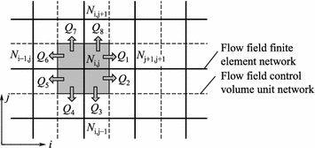

    

    RTM flow field CV/FEM calculation concept

    By calculating the filling coefficient F of the control volume unit, the flow leading edge is determined to be:

    $$ F = \frac{{Q_{\text{r}} }}{V}, $$

    (5.51)

    where Q _r is the resin volume in the N _ij control volume unit at time t; V is the volume of the control volume unit in the N _ij-th control volume unit.

    Hence,

    F = 0::

    no resin flow will occur into this node controlled volume unit. The node will be in an unfilled zone.

    0 < F < 1::

    resin flows into this node controlled volume unit. The node is in the flow leading edge.

    F = 1::

    resin has filled this node controlled volume unit. The node is in the filled zone.

    On the basis of the pressure field at each iteration, the flow leading edge location can be determined by calculating the F values at a specified time, and the entire process of resin flow filling mold in RTM can be calculated.

    If some dry spots are formed during the mold filling, the air pressure in dry spots will depend on the pressure in the impregnating area around the dry spots and the capillary tube pressure:

    $$ p_{\text{a}} = p_{\text{r}} + p_{\text{c}} $$

    (5.52)

    where p _a is the air pressure in the dry spot; p _r is the resin pressure in the impregnated area around the dry spot; and p _c is the capillary tube pressure.

    If the capillary tube pressure can be ignored, the air pressure in the dried spot can be estimated by the universal gas equation:

    $$ p_{\text{a}} = R\frac{{m_{\text{a}} T}}{{(V_{\text{old}} -\Delta V_{\text{flow}} )}} $$

    (5.53)

    where R is gas constant; m _a is the air mass in the dry spot; T is the thermodynamic temperature; V _old is the final effective volume of the dry spot; ΔV _flow is the resin volume flow into dry spots from the surrounding impregnated area.

  • (3) Computer simulation

    • ① Pressure distribution simulation: Resin is injected into molds to fill the mold cavity. If the pressure is too low the resin cannot penetrate the fiber bundle to impregnate the fibers and bubbles will be difficult to remove, extending the mold filling time. If an excessively high pressure is applied, the amount of resin flushing the fiber and mold will be greatly increased, resulting in fiber deformation and resin overflow. By simulating the liquid pressure distribution, the resin flow and mold filling can be predicted. Processing parameters such as the injection pressure can be optimized. The simulated results of the resin flow pressure field can also serve as a basis for predicting the flow advancement and resin/fiber impregnation effectiveness, and for optimization of the mold injection and resin overflow mouths, mold stiffness design, and force applied to the mold. In Fig. 5.55, a simulation of the pressure field distribution at an early injection stage and at the end stage is presented.

      Fig. 5.55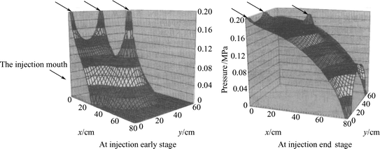

      

      Simulation of pressure field distribution

    • ② Flow leading edge simulation: Computer simulation of the resin flow leading edge can predict the course of mold filling in RTM molding, revealing the flow leading edge location at any time, providing important information on the mold filling time, and the resin blending line. The simulation can also enable visual simulation of the whole process of resin flow and mold filling, as shown in Fig. 5.56. In this Figure, the different gray levels indicate the different resin flow leading edges at any time. Furthermore, flow leading edge simulation can predict possible locations of dry spots as shown in Fig. 5.57. The numbers indicate the flow leading edge locations at specific times.

      Fig. 5.56

      

      Simulation of resin flow leading edge

      Fig. 5.57

      

      Prediction of dried spots in unsymmetrical injection

5.5.3.3 In Situ Process Monitoring

In situ processing monitoring refers to techniques that enable tracking of the cure process in situ in composite manufacturing. Such monitoring can enable optimized pressure application and curing temperature to guarantee the processing quality. The use of this technique can avoid some defects such as resin-rich and resin-starved regions, insufficient curing or over curing, and non-uniform curing can be avoided. In situ processing monitoring has become an important method to improve composite quality stability.

The basic principle of in situ processing monitoring is to place special sensors in the composite layers and determine the resin property changes during the cure process, such as temperature, viscosity, modulus, functional group concentration, and electrical performance. These property changes are recorded and input into a computer. Differences between the cure model and the input signals, allows the cure temperature and pressure to be regulated. This “smart” loop provides continuous automatic control of the cure process to ensure the composite quality.

On the basis of the different sensors used, composite in situ processing monitoring includes dielectric, fiber optic sensor, and thermal couple monitoring. Currently, dielectric monitoring is widely used; however, fiber optic sensor-based monitoring is rapidly advanced in composite processing.

• (1) Dynamic dielectric monitoring

  The principle of dynamic dielectric monitoring is to use special electrode sensors, placed at different positions on the composite to be cured. The sensors measure changes of dielectric properties caused by the resin matrix molecular structure and viscosity changes, which occur during the cure reaction. The measured electrical performance data are used to select an appropriate pressure application time, and adjust for control of the cure temperature.

  Dielectric performance of a resin matrix reflects the ability to store and transmit electrical charge. These features are denoted as the dielectric constant and dielectric loss. The dielectric constant is a material parameter denoting the electrical energy stored when molecular polarization takes place in resin molecules. The dielectric loss is a material parameter denoting the electrical energy loss caused by conductive or orientation relaxation. The polarizations changes of these two parameters will be examined in the following section. 

  • (1) Induced polarization: Induced polarization includes electronic polarization and atomic polarization. Electronic polarization is electronic cloud migration against the atomic core under the action of an electric field, while atomic polarization refers to relative migration between two atomic cores. These two polarization contributions are small in a rapidly changing electric field. These polarizations are synchronous with the electrical field change; hence, induced polarization has a small contribution to both the dielectric constant and dielectric loss.

  • (2) Orientation polarization: Orientation polarization relates to the orientation of polarized bonds with a permanent electric dipole moment under the action of electric field. This type of polarization dominates the dielectric behavior of glassy polymers. If no applied field exists, the orientation of the dipole moment of the polarized bonds will be randomly distributed. When a field is applied, the polarized bonds will rotate and orient along the field direction, i.e., orientation polarization takes place. Polarized bonds must overcome the forces acting between molecules to rotate in the electric field and reach a new equilibrium state. The time needed for this change is called the relaxation time τ, which depends on the polymer molecular structures. Generally, the relaxation time increases as the cure degree increases. Let the alternating field frequency be f. When τ ≤ 1/f, the dipole moment will take an orientation synchronous with the field because the stored energy in polymers in a charge-half cycle will be totally released in the discharge-half cycle. Although there is energy exchange between the polymer and the field, no energy loss will occur. The polymer will become highly polarized under such circumstances, giving a high dielectric constant without any dielectric loss. When τ ≈ 1/f or τ > 1/f, the orientation of the dipole moment is delayed with respect to the electric field change. The polymer polarization will gradually decrease resulting in a lower dielectric constant. Simultaneously, because the energy absorbed by polymers is less than the released energy, strong dielectric loss will occur. When τ >> 1/f, the orientation of the dipole moment cannot follow the field change and no polarization will occur. In this case, both the dielectric constant and loss tend to zero. Hence, resin cure information can be derived from the response of the dielectric constant and loss to a permanent electric field.

  • (3) Ion migration: Ion migration refers to the movement of impurity ions in the resin under an applied electric field. This effect can give the resin a certain conductivity. Note that the material ion conductivity will be inversely proportion to viscosity over certain ion concentration and temperature ranges. Ion migration can only occur when resin is in a viscous state. This correlation can enable the resin viscosity during the curing process to be monitored by measuring ion conductivity.

    In summary, if the dielectric constant of a resin matrix can be monitoring during the composite curing, information on resin viscosity and chemical structure changes can be obtained. For thermosetting resins that show a flow state at high temperature before gelling, the resin viscosity can be evaluated by analyzing the changes in ion conductivity. After gelling, the loss factor will mainly depend on the polarized orientation, which can be used to evaluate changes in the chemical structures. In Fig. 5.58, the resin ion viscosity change curve of the T300/QY8911 material system during curing is given, indicating the viscosity change mode of thermosetting resins at the early curing stage. Figure 5.59 is the loss factor change curve of this material system in the curing dwell time reflecting the increase in dielectric relaxation time caused by matrix resin cross-linking, which decreases the loss factor.

    Fig. 5.58

    

    Logarithm ion viscosity change curve of T300/QY8911 during curing

    Fig. 5.59

    

    Loss factor change curve of T300/QY8911 in curing dwell time

    Dielectric monitoring can provide information on composite resin matrix viscosity and chemical structure changes occurring during curing process. This information is useful for performing curing processes under in situ monitoring; however, in practical applications, this technique is somewhat limited.

    First, when resin is in the viscous-flow state, the ion conductivity will be subject to many influences, and the resin viscosity change can cause ion activity to increase, resulting in a different ion conductivity. However, other influences exist and there will not be a simple correlation between the ion viscosity based on the ion conductivity and the real resin viscosity or traditional shear viscosity. In practical monitoring, it can be assumed that the ion concentration and ion charges will remain unchanged in the same sample; hence, the conductivity change will be mainly caused by the viscosity change, and the ion change modes can reflect the real sample viscosity change modes. However, as mentioned earlier, the ion conductive behaviors of polymers are mainly caused by impurities in the materials. There will be a difference in the ion concentrations and as a result, the ion viscosity change curve derived from different monitoring methods cannot be used for quantitative comparison of the material’s real viscosity.

    Furthermore, it should be noted, in thermosetting resin matrix curing process, the ion viscosity value before the gel point can reflect the real viscosity change mode. After the gel point, the ion viscosity will no longer show a change and will rapidly tend to an infinitely large value and then gradually stabilize.

• (2) Fiber optic sensor monitoring

  Fiber optic sensor monitoring systems consist of an optic transmitter, sensor element, optic receiver, and signal processor. The basic principle is to use a special optic fiber as a sensor, which is embedded into to composite or structure to be cured. The optical system can then be monitored during the in situ cure process. Optic fiber sensors have the advantages of small size, high sensitivity, and good compatibility with resin matrices. On the basis of different monitoring mechanisms, fiber optic sensors can be divided into the following types.

  • (1) Fiber optic refraction sensing: In composite resin matrix cure process, during the molecular cross-linking reaction, the ratios of different chemical bonds will change. Because each chemical covalent bond has different refraction coefficients, the changes in chemical bonding during curing will result in changes of the resin refraction. Thus, by monitoring changes of the resin refraction, information on the resin cure degree can be obtained. Fiber optic refraction sensors are designed based on this principle.

    There are many types of fiber optic sensors available and a typical construction shown as in Fig. 5.60. The refractivity n ₁ of the optic fiber core layer is slightly greater than that of the cladding layer n ₂. Total refection will take place at the interface between the core layer and the cladding layer and light will be transmitted along the optic fiber core. If a section of the cladding layer (2–3 mm) is removed the exposed fiber core section will become the optical sensor in the composite curing monitoring technique. The fiber can be embedded into composites and light refraction will take place at the interface between the fiber core and resin, resulting in the loss of some light energy and light attenuation. Tracing of the optic energy change can give information on the resin cure degree.

    Fig. 5.60

    

    Schematic of optical refraction sensor

    An optic cure sensor system based on resin refraction measurements is simple in construction. Usually, a monochromatic light source is used. At the light measurement end, the change of the light energy is measured. Hence, this is an economical and practical approach to monitoring. However, in most cases, special optic fibers with a high refraction fiber core should be used, and can only qualitatively give information of cure reaction process. Furthermore, the refraction measurement range is limited. Another issue to consider is that resin refraction correlates with density, while density is largely dependent on the effects of temperature. Outside of ambient temperatures the measured resin refraction change will show the combined effects of cure degree and temperature. Thus, it is difficult to evaluate the cure degree change only from the refraction change. This monitoring approach is only suitable for measuring the cure degree during a dwell time in a curing process.

  • (2) Infrared spectroscopic sensing: In infrared spectroscopic sensing, infrared light absorption by characteristic resin functional groups is used to determine the change of functional group content in the resin. The characteristic peak location and intensity relate to a specific functional group, and the peak intensity can be used to monitor its concentration change and determine the curing degree. For example, in an epoxy resin system, the cross-linking functional groups are epoxy groups. The characteristic peak change of the epoxy group can be analyzed to determine the cure degree of the composites. This information can be used to control the pressure application time and curing temperature. Infrared spectroscopic sensors include fiber optic infrared absorption sensors and evanescent wave sensors.

    In fiber optic infrared absorption sensors, two optic fibers with an end distance of 0.5–1.5 mm are oriented in the same direction and embedded into prepregs. The two free ends of the fiber are connected with a monochromatic scanner and an infrared spectrometer. Once the cure reaction is initialed, the resin viscosity will increase and resin will flow into the gap between the two fiber ends. Infrared light will produce characteristic absorption peaks when passing through the resin layers. At the receiver end, the resin absorption spectrum can be analyzed. On the basis of the Beer–Lambert law, a series of resin infrared absorption spectra are collected at certain time intervals. Quantitative measurements of the epoxy, oxyhydrogen, and amine group concentration can allow the cure rate and degree to be determined.

    Fiber optic evanescent wave sensors are another type of cure monitoring sensor based on analysis of infrared absorption spectra. The construction of this type of sensor is similar to that of the fiber optic refraction sensors shown in Fig. 5.60; however, the sensor section is longer than that of the evanescent wave sensor (approximately 20 cm). In cure monitoring, as the resin viscosity decreases, the optical evanescent wave will dissipate at the interface between the fiber core and resin. The absorption spectra measured at the light receiver can allow dynamic cure reaction information to be determined. In optic fiber evanescent wave sensors, a special optical fiber with a high core refractivity is required, which gives low sensitivity.

    Fiber optic cure monitoring sensors based on infrared spectral analysis can quantitatively determine the cure degree; however, a wide band light source and complicated spectrometer are needed together with complex data processing, which adds to the cost of this approach.

  • (3) Fiber optic bend sensor: In applications of optic fibers, the fiber axis undergoes periodic bending on a micrometer scale caused by non-uniform pressure. Fiber optic bending can cause increased losses, resulting in energy dissipation during light transmission. The reason for this is that small periodic bending causes repeated coupling between the transmitting and radiation moduli, resulting in some light energy of the transmitting modulus radiating outside of the fiber core.

    In composite prepregs, reinforced fibers have a defined density. The load on fibers will change at different times in the curing process. The pressure transmitted to the fiber sensor section will also change, which will change the degree of fiber microbending and the resulting minor bending loss. In composite autoclave processing, test results indicate that fiber bending sensors can be used to accurately determine the lowest viscosity point and completion of a curing process with good reproducibility. The sensitivity is related to the pressure field in the curing process.

    In the use of fiber optic bending sensors to monitor composite cure process, it is important properly place the fiber based on the selected prepregs. This method has simple equipment requirements, is practical, and its results can be easily translated into production.

  • (4) Bragg grating sensors: Bragg grating sensors have developed rapidly in recent years. In Bragg grating sensors, light wavelength coding is used for signal transmission, which can overcome fluctuations in the light energy output as well as losses of the fiber connectors and coupler. Wavelength multiplexing and quasi-distribution measurements can be performed in a single fiber.

    The basic principle of a Bragg grating sensor is the Bragg wavelength measurement. The Bragg wavelength λ _B correlates with the fiber effective refraction n _eff and the period of a refraction grating A, as shown below:

    $$ \lambda_{\text{B}} = 2n_{\text{eff}} \varLambda . $$

    (5.54)

    When Bragg grating sensors are embedded in a composite resin matrix, the resin is strained and thus causes optical elastic effects, which can result in changes of n _eff and $\varLambda$. These effects produce a Bragg wavelength displacement. A modulator can be used to measure the Bragg wavelength displacement from which, the strain can be determined. Bragg grating sensors can be used to monitor composite autoclave processing. From a curve of the change of the Bragg wavelength vs time, the material changes can be tracked. Furthermore, the glass stage of the resin curing and some defects such as debonding and cracking in the measured zone can be identified.

    Applications of Bragg grating sensors face a cross-sensitivity problem, i.e., the grating is sensitive to both stress and temperature. When the grating is used for measurements, it is difficult to determine whether a change of the Bragg wavelength is caused by stress or temperature. In practical applications, it is necessary to take some measures to compensate or identify these differences.

    Two in situ monitoring methods used in process are introduced above. Composite processing occurs under closed conditions. Knowledge of the processing parameters is the only way apply in situ monitoring. To properly select processing parameters, it is necessary to collect as much useful information as possible.

• (3) Data types in monitoring

  The first issue in in situ monitoring of composite processes to collect a large volume of curing information. Typically, three types of data on the process are collected: first condition parameters of the equipment; second, temperature and pressure data, which can indicate a material’s curing conditions; third, information about the physical and chemical structure changes taking place in the materials during the curing process.

  • (1) Equipment condition: The equipment condition is a very easily measured parameter. In most cases, the control of composite production is performed based on control of the equipment, such as the location of a filament winding head, winding speed, fiber tension, together with mandrel torsion moment, speed, and temperature. These parameters should remain consistent over different production cycles. Improper control will cause product quality problems.

  • (2) Temperature and pressure: There are two types of temperature parameters, one is the directly controllable ambient temperature data, such as the heated air temperature in autoclave composite curing or the press molding plate temperature. The temperature conditions represented by these types of data will be directly controlled by a temperature control unit in the composite curing process. These values will be compared and maintained consistent with the preset control program. Another type of temperature data is indirectly controlled ambient temperature data, which reflects the actual temperature conditions. These depend on the controllable temperature, but are not direct controlled. It is difficult to maintain high consistency of these temperatures with a preset control program. For example, the mold temperature in composite autoclave curing is indirectly controlled by the air temperature inside the autoclave. However, it is very difficult to ensure accurate control of this temperature. In addition, the temperature inside the composite part can only be indirectly controlled by the external temperature control unit and is affected by the reaction heat generated during curing process. Hence, temperature is one of the more difficult parameters to control.

    The pressure data reflect the pressure conditions induced on the composites during curing. The pressure conditions include the applied processing pressure, such as the air pressure in the autoclave, the plate pressure in press molding, and the actual pressure resin and fibers are subjected to. Only the pressure induced to the resin can contribute to air bubble removal. In vacuum bag curing processes, the pressure data include both the applied positive pressure and the pressure produced by the applied vacuum.

  • (3) Conditions of cured material include resin matrix cure degree, resin viscosity, fiber tension force, and fiber positions.

    Ideal curing processes require that the cure reaction of the resin matrix be performed at the programmed speed, to avoid rapid curing, which might result in product quality problems, or excessively slow curing, which will increase the production costs. To achieve an optimal curing program in situ data of the cure degree related to the change of chemical structure of the resin matrix are collected during curing. To avoid mistakes in selection of the pressure application time, it is necessary to perform in situ monitoring of the resin viscosity change. Pressure applied when the resin viscosity is too low will cause resin out flow and the pressure will quickly decline and the resulting composite will not be well compacted, and may feature resin-starved regions. If pressure is applied too late, internal air bubbles cannot be removed completely contributing to void defects.

• (4) Creation of monitoring system

  Composite in situ processing monitoring systems can be built-up with different methods combined with a computer. On the basis of the collected data, in situ monitoring of processing parameters such as temperature and pressure can be performed to guarantee the product quality. A typical autoclave curing monitoring system is shown as Fig. 5.61, which is composed of three parts.

  Fig. 5.61

  

  Typical autoclave curing monitoring system

  • (1) Data collection system in autoclave: This system can monitor the autoclave internal air temperature, pressure, part temperature, and material viscosity and chemical structure determined by dielectric or fiber optic sensors. These data are transferred to a computer processing system.

  • (2) Computer decision system: The program module in the computer system can use the collected in situ processing monitoring data from the resin curing process. The temperature, cure degree, residual stress, and part deformation under curing of each layer can be analyzed and compared with available data and knowledge to obtain optimized processing parameters for further implementation. The analysis results can be displayed for evaluation and inspection.

  • (3) Control system for curing parameters: This kind of system can use collected information from curing monitoring together with calculation results provided by an analysis module to drive the actuating unit in the controller cabinet and automatically adjust the processing parameters.

• (5) Problems in monitoring techniques

  Currently, some problems exist for in situ process monitoring of composite part production, including:

  • (1) Measurability: no ideal sensors are available that can provide information on both the physical and chemical changes occurring during composite curing. Not all requirements for material conditions, such as prepreg status and processing conditions (closed vacuum bag/autoclave conditions) can be determined during the composite part manufacture. Apart from traditional temperature and pressure sensors, all sensors used in part production monitoring can only provide information on trends of material viscosity and the curing reaction.

    Temperature and pressure sensors can only give information at specified points in materials and full data on each section is difficult to acquire. To collect more curing parameter information from important areas, more sensors will need to be placed inside the composite parts.

    Disturbances may cause some problems in data collection and the signal collection may vary over time. Hence, small fluctuations may lead to a discontinuous curve.

  • (2) Feasibility refers to the ability to control the output of a specified value in a given time.

    Measurement of output or process parameters with high spatial and temporal resolution is necessary but the control system should also have enough accuracy to enable control of parameters at different locations on a part. For example, one set of autoclave curing monitoring systems can inspect the distribution of the whole curing status inside a composite part. A computer analysis system can acquire the vector output of the processing parameters from the whole part. Common autoclave input control parameters are limited to temperature and pressure. Furthermore, only control of the air temperature inside the autoclave can be achieved, which may not be consistent with each of the processing parameter and analyzed results. Owing to the large heat inertia of an autoclave, tools, and the part itself, the process control cannot be performed with high time resolution.

    To achieve consistency between measurements and controls, the heating molds should have multiple independent temperature control zones, so that independent heat input can be applied to different sections of the composite and the spatial resolution can be improved.

  • (3) Low cost: The use of sensors will increase the complexity of part packing before curing. In particular for fiber optic sensors, because of their brittleness, which requires special treatment before use. This is will increase the work involved in packing and production costs.

    Sensors are mostly single-use elements; hence, the part cost should include the sensor cost. Thus, in situ processing monitoring system should be based on low-cost sensors that are easy to install.

  • (4) Compatibility: The sensors are embedded into the composites, and many of them will be remain inside the part for long time. The sensor materials should not influence the part curing behavior or produce additional defects in service. For materials and sensors to be used, it is necessary to inspect the effects of sensors on mechanical performance of the material to evaluate the compatibility between the sensors and material system.

5.5.3.4 Statistical Processing Control

Statistical processing control (SPC) is a kind of output control method, as shown in Fig. 5.62. In this control method, sampling, quality inspection, and statistical analysis of results are performed for composite products to determine and eliminate factors that cause quality problems. The feedback of this information forms a control loop, to realize the needs for quality control and quality improvement.

Fig. 5.62

SPC control principle

Fluctuations of composite properties and shape can be divided into normal and abnormal fluctuations. Normal fluctuation is generated from the unavoidable factors occasionally encountered during processing. These factors have less effect on the product quality and are technically or economically unfeasible to eliminate. Abnormal fluctuations are caused by system abnormities and have a pronounced effect on product quality. These can be avoided and eliminated by proper counter measures. SPC involves the use of statistical analysis to identify random and abnormal fluctuations of product quality in production. This allows precautions to be taken for possible abnormities in production.

• (1) Statistical analysis methods

Statistical analysis is the basis of SPC, and includes many methods such as control charts, bar graphs, scatter diagrams, processing ability indices, and relative and regression analyses. Some of these methods will be discussed in the following:

• (1) Control chart: A control chart is a kind of statistical graph used to monitor measure, diagnose, and improve processing conditions. A sample’s statistical results are ranked in a certain sequence, as shown in Fig. 5.63. In general, these results include an upper control limit (UCL), lower control limit (LCL), and a central line (CL). The central line typically represents the average sample value, while the upper and lower control limits depend on the quality stability requirements. In a regular inspection, if the sample value is higher than the UCL or lower than LCL, it can be concluded that abnormal conditions were present in production.

  Fig. 5.63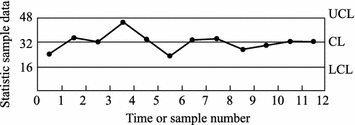

  

  Schematic control chart

  Current control charts include percentage control charts for rejected products, number control charts for rejected products, and defect ratio and defect number control charts.

• (2) Bar graph: Bar graphs show data distribution features, which can be used to directly display a data distribution.

• (3) Ranking graph: also known as Pareto figure, involves ranking the effects of each items from the most to the least important. It can be used to identify the primary, secondary, or common problems that affect product quality. The primary factors can be detected and quality improvements methods suggested.

• (4) Scatter diagram: the data point distribution is used to show the relationship between variation and to reveal and display the correlation between two sets of data or confirm and predict the correlation.

• (5) Relative analysis is used to study the relationships among variations and assumes that all variations change randomly at the same positions without separation from the primary and secondary ranks.

• (2) Data collection

To acquire accurate and reliable statistical data, systematic sampling should be conducted. The sample selection should be continuously and randomly performed, where the randomicity prevents unintentional selection of a sample. The samples should be representative of the materials. The sample data should be continuously accumulated so that the effects of factors that occur regularly can be determined. In this way, performance degradation in a production system can be recognized, serving as a reference for system optimization.

There may be many factors to inspect in one product and it is impossible to check and analyze all of them. Only key parameters that can give insight into the processing should be measured. Once the data are collected, the data should be processed into figures or curves based on statistical approaches. A table of the data alone is not be sufficient to indicate changes in regularity, even in the case of only a few data points to be analyzed. In most cases, it is necessary to use the same data in different analyses to determine correlations among different factors, or time-dependent trends.

• (3) Implementation of SPC

In practical applications, the implementation of SPC should be performed in two steps: first the analysis stage, second the control stage.

In the analysis stage, preparation for production should be performed, following certain standards, to ensure the raw materials, labor, equipment, and measurement systems are in place before production can be started. The production should be performed under conditions that minimize any abnormities in analysis stage. Calculation of the control limits is based on the data collected in production, which is used to produce control graphs and bar charts. Process ability analysis can also be performed to check if the production is within a statistically stable state or not. If any single factor cannot be satisfied, the causes should be investigated and steps taken to improve the process before restarting the production preparation and analysis. If the requirements of the analysis stage are satisfied the analysis stage can be terminated allowing for advancement to the SPC control stage.

In the control stage, control graphs and other charts are used for monitoring production. In this stage, the control limits in control graphs are determined based on the analyzed results in the analysis stage. The data collected in production should be used in control graphs at the same time. The control graphs should be closely observed, and data fluctuation in control graphs will show whether the production is under control or not. If production is out of control, the causes should be identified and eliminated as quickly as possible.

In practical applications, each control item should proceed though the above stages, and the processes from analysis to monitoring should be repeated if necessary.

• (4) Advancement of SPC

SPC is a new quality management system and not yet widely used in composite process control in China. However, SPC has been widely applied in other industries such as the electronic industry, and various types of computer software have been developed and applied to in situ process monitoring. SPC methods show good potential for overcoming the difficultly of composite processing control.

5.5.3.5 Experiential Control Methods

Experiential control method, also called trial-and-error methods, use experiences gathered over long-term production to decide the processing technique, or the use of simple specimens for testing and qualitative analysis of products. This method is only suitable for a narrow range of composites and is not applicable if the material and shape of the products changes. In these cases, repeat testing is necessary, resulting in a long production cycle and high costs. Hence, this method is not currently widely used in production.

5.5.3.6 Processing Quality Inspection

Whatever processing quality control method is used, it is necessary in quality assurance to inspect and track the processing quality. The quality assurance department is responsible for checking if production is performed under the specified specification. The work involved in processing quality inspection will be discussed in the following section:

• (1) Raw material inspection

The following items should be included in raw material inspections.

• (1) Verify the raw material’s name, grade, supplier and product series number, and perform tests on the key performance parameters to ensure quality.

• (2) Regularly inspect material storage and packages to avoid material degradation, damage, corrosion, and misidentification caused by storage problems or package breakage.

• (3) Recheck the contents in item (1) before using a material, verify that degradable materials, such as prepreg and adhesives are within the specified shelf life.

• (4) Check the records of the source, storage, and treatment of material that have already been used.

• (2) Equipment and tools inspection

Equipment in good condition is essential to produce high-quality composite products. Before operation, all equipment, such as autoclaves, winding machines, and prepreg tape placing machines, should be carefully checked and calibrated. In production, use of the equipment should be recorded with their operating conditions. Equipment should be regularly maintained to ensure good condition. Problems should be identified and repaired any in a timely manner.

Molds should be checked and verified according to specifications. The molds should be guaranteed to give products that can satisfy the design and the technical specification requirements based on the correct use of the materials processing techniques. The mold surface should be checked before use to guarantee a clean surface without any corrosion or damage.

• (3) Production condition inspection

The inspection of composite production environment is also part of an inspection program. In a controlled environment, uncontrolled spray, exposing to dust, smoke, oil vapor, or any other chemical substances or grains that may affect processing, is prohibited. A clean laying-up room should be used with normal air filtering under positive pressure conditions.

• (4) Processing flow chart inspection

In composite part laying-up and curing processes, certain key operation steps should be strictly controlled. These steps should be clearly indicated in the specification and guaranteed by inspection.

• (1) Check the release agent applied to the mold surface and its cured condition.

• (2) Check the prepreg laying-up to guarantee the correct layer number and orientation.

• (3) If core materials are used, check their correct splicing position.

• (4) Check the correct processing display and records.

• (5) Check the production records including:

  • ① Material supplier, data, series number, batch number, and the storage time in shelf life.

  • ② Processing parameters including applied pressure, temperature, heating-up rate, dwell time.

  • ③ Autoclave or heating chamber series number.

  • ④ Part or product series number.

(Translated by Jianmao Tang)

References

ASTM D6264-07 (2007) Standard test method for measuring damage resistance of fiber-reinforced polymer-matrix composite to concentrated quasi-static indentation force
ASTM D 7136-07 (2007) Standard test method for measuring the damage resistance of a fiber-reinforced polymer matrix composite to a drop-weight impact event
ASTM D7137-07 (2007) Standard test method for compressive residual strength properties of damaged polymer matrix composite plates
FAA AC 20-107B (2003) Composite aircraft structure (draft)
HB 7618-2009 (2009) Data presentation guidelines on mechanical properties for polymer matrix composite materials (Revised edition, in Chinese)
McCarvill W, Ward S, Bogucki G, Tomblin JS (2003) Guidelines and recommended criteria for the development of a material specification for carbon fiber/epoxy unidirectional prepregs. DOT/FAA/AR-02/109
MIL HDBK-17-1F (2002) Composite materials handbook Vol 1. Polymer matrix composites guidelines for characterization of structural materials
Shikhmanter L, Cina B, Eldror I (1991) Fractography of multidirectional CFRP composites tested statically. Composites 22(6):437–444
Shen Z, Chai YN, Yang SC et al (2006) The Outline of new specifications on strength of composite aircraft structures (In Chinese). Acta Aeronaut Sinica 27(5):784–788
Shen Z, Yang SC, Chen PH (2007) Behaviors of composite materials to withstand impact and structural compressive design allowables (in Chinese). Acta Aeronaut Sinica 28(3):561–566
Shen Z, Yang SC, Chen PH (2008) Experimental study on the behavior and characterization methods of composites to withstand impact (in Chinese). Actamater Compos Sinica 25(5):125–133
Shen Z, Yang SC (2007) Property requirements of composite systems applicable to aircraft structures (In Chinese). J Mater Eng China SAMPE 248–252
Tomblin JS, Ng YC, Raju KS (2003) Material qualification and equivalency for polymer matrix composite material systems: Updated Procedure. DOT/FAA/AR-03/19
Author information
Authors and Affiliations
Corresponding author
Editor information
Editors and Affiliations
Rights and permissions
Copyright information
© 2018 Chemical Industry Press, Beijing and Springer Nature Singapore Pte Ltd.
About this chapter
Cite this chapter
Zhang, Z., Zhang, Z., Shen, Z., He, S., Li, Y., Chao, M. (2018). Composite Property Testing, Characterization, and Quality Control. In: Yi, XS., Du, S., Zhang, L. (eds) Composite Materials Engineering, Volume 1. Springer, Singapore. https://doi.org/10.1007/978-981-10-5696-3_5
Download citation
DOI: https://doi.org/10.1007/978-981-10-5696-3_5
Published:
Publisher Name: Springer, Singapore
Print ISBN: 978-981-10-5695-6
Online ISBN: 978-981-10-5696-3
eBook Packages: Chemistry and Materials ScienceChemistry and Material Science (R0)