Policy Simulation: Macroeconomic Effects of Slowdown in Private Investment Growth

Abstract

In the first half of 2016, China’s private investment growth dropped sharply, triggering concern and heated discussion among policymakers and scholars. Given the easing monetary policy implemented especially in the first quarter, what made the private investment growth plummet? Some clues may be found by analyzing changes in shares of private investment in total FAI by industry.

These keywords were added by machine and not by the authors. This process is experimental and the keywords may be updated as the learning algorithm improves.

3.1 Background

In the first half of 2016, China’s private investment growth dropped sharply, triggering concern and heated discussion among policymakers and scholars. Given the easing monetary policy implemented especially in the first quarter, what made the private investment growth plummet? Some clues may be found by analyzing changes in shares of private investment in total FAI by industry (see Table 3.1).

Table 3.1 Shares of private investment in total FAI by industry (%)

First, in the first half of 2016, impacted by the dramatic fall in the private investment growth, the ratio of private investment to total FAI declined to 61.46%, from 65.13% in the same period a year earlier, down by 3.67 percentage points. On a similar comparison, the ratio in the tertiary industry decreased from 30.43 to 28.39%, down by 2.04 percentage points, contributing 55.66% of the decline. The ratio in the secondary industry dropped from 32.60 to 30.77%, down by 1.83 percentage points, contributing 49.98% of the decline. And the ratio in the primary industry increased by 0.21 percentage points (see Table 3.1). Therefore, the decelerating investment growth in the second and tertiary industry is the key factor to explain the significant drop in the private investment growth.

Second, as to the secondary industry, the ratio of private investment to total FAI in production and supply of electricity, gas and water, did not fall but rise, from 1.62% up to 1.90%. As shown by Table 3.2, after 2012, the ratio kept rising steadily, suggesting that in the urban public infrastructure and services sectors, there is no evidence that the private investment has been crowded out, though the proportion of private investment is relatively small. In the first half of 2016, the key factor to explain the decline of the ratio in the secondary industry is the decelerating private investment growth in manufacturing and mining, where the former contributing 95.09% of the decline, and the latter contributing 17.43%. It is noteworthy that the decline of the ratio in mining did not first took place in the first half of 2016 but after 2012, though it is true that the decline has expanded since early 2016.

Table 3.2 Shares of private investment in the secondary industry by sector (%)

Furthermore, in terms of subsectors of manufacturing, ratios of private investment to the FAI in non-metallic minerals, ferrous metals and non-ferrous metal smelting and pressing processing were down by 0.38, 0.04 and 0.14 percentage points respectively, in total contributing 32.59% of private investment growth in manufacturing. Ratios in general-purpose machinery and special-purpose machinery manufacturing fell rapidly as well, contributing 10.53 and 13.61% of the decline in private investment growth in manufacturing. As some of most valuable equipment has been installed in general-purpose machinery and special-purpose machinery manufacturing, such as mining, metallurgy, construction, metal processing, and so on, the decline of the ratios in these two sectors may also closely related to the private investment’s exit from these sectors, besides, affected by the government’s measures to constrain the capacity in these sectors (see Table 3.3).

Table 3.3 Shares of private investment in manufacturing by sector (%)

Thirdly, as to the tertiary industry, the share of private investment in the FAI in transport, storage and post declined to 2.06% in the first half of 2016, from 2.20% in the same period last year, down by 0.14 percentage points, contributing 6.96% of the decline. The share in water, conservancy, environment and public facilities only slightly declined by 0.01 percentage points, contributing 0.63 of the decline. The shares in education and health and social work, did not fall but rise, up by 0.03 and 0.04 percentage points respectively. The shares in culture, sports, and entertainment, together with public management, social securities, and social organizations, declined slightly as well, contributing very few to the decline (see Table 3.4). By contrast, the shares in these six sectors in the first half of 2015 were all up over those in the same period a year earlier. Nevertheless, the private investment in these sectors only accounts for 22.23% of the total in the tertiary industry, suggesting that changes in the private investment in these sectors are not the main factors to determine the changes in the tertiary industry. The main factors may lie behind the changes in other sectors in the tertiary industry.

Table 3.4 Shares of private investment in the tertiary industry (%)

As data on the private investment in other sectors in the tertiary industry are not available, we cannot find out which sectors are the main forces to determine the decline in private investment growth directly. However, the following evidence may be helpful.

• 1. According to the Classification of Sectors of China’s National Economy (GB/T 4754-2002), excluding the above mentioned six sectors, the rest of sectors in the tertiary industry are: wholesale and retail trades, information transmission, computer services and software, finance, real estate, leasing and business services, scientific research, technical services and geologic prospecting, and services to households and other services. It is some of these sectors that contributed 88.66% of changes in the decline of private investment growth in the tertiary industry in the first half of 2016.

• 2. Among the above mentioned seven sectors, wholesale and retail trades, together with the private investment in real estate, are two major sectors. Take real estate for example, the domestic investment in real estate development reached 8.66 trillion yuan in 2014, and investment from the state-owned and state holding enterprises (SOEs) and the collective-owned enterprises in total accounted for about 85% of the total, most of the rest was private investment.

• 3. In the first half of 2016, as the growth of the total retail sales of consumer goods stayed stable, the private investment in wholesale and retail trades would not change too much, suggesting that changes in the share of the private investment in real estate be the major determinant to the decline of private investment growth in the tertiary industry. As shown by Fig. 3.1, in June, 2015, for real estate development, the growth rate of the investment from the SOEs went up sharply from 2.7% at the end of 2015 to 17.0% in January, 2016, overtaking that from the total FAI for the first time, while in the same period the rate of property investment only slightly rose from 1.0 to 3.0%, suggesting that the relatively lower growth rate of the investment from non-SOEs dragged down that of total investment. On account of this, the share of investment from SOEs rose from 15.0% at the end of 2015 to 16.6% in June, 2016, 2.0 percentage points higher than that in the same period a year earlier.

  Fig. 3.1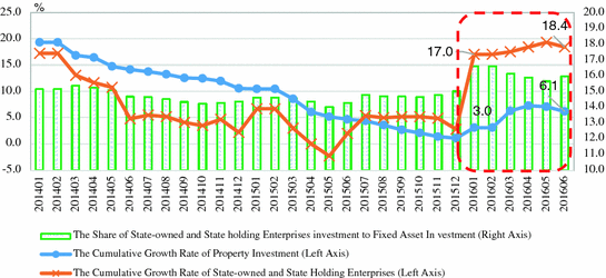

  

  Growth rates of property investment from SOEs. Source CQMM team calculations on CEIC data

Furthermore, in terms of incremental funds in the real estate development, in the first half of 2015, the investment increased by 193.6 billion yuan over the same period a year earlier, and the share of investment from SOEs was only 6.01%. By contrast, in the first half of 2016, the investment increased by 267.6 billion yuan over the same period last year, and the investment from SOEs grew by 115.4 billion yuan, accounting for 43.1% of the total increment.

In summary, the dramatic drop in the share of private investment in total FAI is attributable to the following two direct causes:

First, the private capital accelerated to exit from those manufacturing sectors with overcapacity, and in the meantime, due to technology barrier, shortage of funds, or entry barrier, the private capital was not able to enter into some high-end manufacturing sectors and some quasi-public services, leading to decelerating growth of private investment. These exiting funds turn to invest in the fictitious economy, such as commodity futures, housing markets in upper-tier cities, dollars markets, gold markets, and so on. In addition, some of them outflew, making the growth rate of OFDI accelerated significantly in the first half of 2016.

Second, the growth rate of private investment in real estate in the first half of 2016 did not rise significantly, dragging down its share in real estate investment, while the share of the SOEs’ investment climbed correspondingly. One cause is that, owing to the bank credit preference and the relatively high fund entry barrier, private capital, which endowed with limited funds and other resources, didn’t have the capability for competing with the SOEs in upper-tier cities, making incremental private investment really limited. The other cause is that most private capital was concentrated in lower-tier cities, where the property market is facing the pressure from destocking, making private capital reluctant to increase investment. Therefore, the fact that the private investment growth dropped dramatically in the first half of 2016 reflects the serious regional divergence of real estate. During the period that property boom in upper-tier cities coexisting with great pressure of destocking in lower-tier cities, it is hard for private capital to challenge the SOEs.

3.2 Further Research

The above analysis suggests that the slowdown of private investment growth is closely related to current supply-side structural reform. On one side, the action to cut overcapacity accelerated, making private investment exit from the relevant sectors. On the other side, during the period that property boom in upper-tier cities coexisting with great pressure of destocking in lower-tier cities, private capital was crowded out by more powerful SOEs. All these reflect that there are at least two weaknesses in current supply-side structural reform. The first is that the measures taken so for to curb overcapacity emphasized too much on the quantity but not the quality. And the result is that, though some excess capacity had been cut, it is difficult for the exiting capital to enter into some more profitable real economy. The second is that the measures to cut overcapacity cannot eliminate those real zombie enterprises by market mechanism, but by government mandates, the latter discarding as useless some more productive capacity owned by private enterprises. Furthermore, the market mechanism does not work well even in those competitive markets. The SOEs, with their credit endorsed by the government, are always easier than private businesses to enter into the capital markets, resulting in virtually unfair competition. And thus, in order to increase effective investment while curbing excess capacity, it is necessary to make some adjustment on the current reform.

In our opinion, the keys to the supply-side reform include: return to the markets, increase the returns on investment (ROI), and stimulate investment and allocate resources according to the market.

Actually, the slowdown of private investment growth is not a new problem which occurred this year. Since 2012, the year in which statistical data on private investment for the first time released, the private investment growth has kept decelerating, owing to the decline of ROI in real economy. The ROI in the first and second quarter of 2016 continued this downward trend, but no sudden fall took place (see Fig. 3.2).

Fig. 3.2

ROI of industrial enterprises. Note (1) ROI = (gross profit − income tax)/(total assets − total liabilities) = (gross profit × 0.75)/(total assets − total liabilities). (2) Data are seasonally adjusted. Source CQMM team calculations on CEIC data

The ROI is an indicator that reflects business operation efficiency comprehensively. There are many factors that affect the ROI, including Assets, liabilities, the gross profit, the corporate income tax, and so on. As Assets, liabilities, and the gross profit, are all determined by businesses, the only factor that the government is able to determine directly is the taxation system. China’s current taxation structure takes the indirect tax, such as value-added tax (VAT) and consumption tax, as the main body. Such structure is not help for business operation and reinvestment, especially during economic recession. When the goods market is not clearing, it is hard for business to shift the tax burden to consumers at the low stream, making businesses have to bear much of the operating tax burden. Besides, much of fees and charges in the social insurance system are mostly put on the businesses. And the result is, the worse is the economy, the greater are the tax burden and cost pressure put on businesses. From this perspective, we suggest that, during economic slowdown, in order to improve their ROI, the government should help businesses reduce their costs and burdens by tax cut and fees and charges reduction. And this would be an effective approach to solving the problem of decelerating investment growth, especially the problem of dramatic drop in private investment growth.

In the next section, the CQMM is used to evaluate the macroeconomic effects of improvement on the ROI.

3.3 Policy Simulation

3.3.1 Model Specification Adjustment

In order to simulate effects of improvement on the ROI, the original CQMM was made some adjustments. The major adjustments are mentioned as follows:

First, equations in the investment module are revised. The investment equation in the original model was specified by the FAI from various sources of funds, not including the FAI from private and non-private investment. In the new equation, the FAI are classified as the private investment and the SOEs’ investment to explain gross capital formation and GDP. As current statistical data based on surveys can only be used to measure the ROI of industrial enterprises, we introduced the variable of private investment in industrial sectors as the intermediate indicator of variable of private investment. In addition, in order to distinguish the private investment and the SOEs’ investment, we assume that the ROI of industrial enterprises can only affect the private investment in industrial sectors, but cannot affect the SOEs’ investment (see Fig. 3.3).

Fig. 3.3

Conduction route of the ROI on private investment

Secondly, for convenience, the ROI variable is assumed as exogenous, its conduction route is mainly via tax adjustment, including the decline of taxes less subsidies on production and imports, and the decrease of income tax. It is noteworthy that the tax adjustment usually has endogenous effects on different modules of the model. For we have studied the effects of tax adjustment in the previous report based on CQMM, it is reduced to exogenous changes on this report.

3.3.2 Simulation Scenarios Planning

Based on the estimated ROI of industrial enterprises, two scenarios are designed as follows:

In Scenario 1, the ROI of industrial enterprises in 2014, 2015, and the first half year of 2016 are kept same as that in the same period of 2013.¹ The aim of this scenario simulation is to evaluate the effects of improvement of ROI on major macroeconomic variables.

In Scenario 2, the situation becomes worse. The ROI of industrial enterprises dropped sharply in 2014, just as in 2015. In 2015 and 2016 they are kept same as that in 2014. The aim of this scenario simulation is to evaluate the macroeconomic effects of continued decline of ROI.

Detailed differences are shown by Fig. 3.4.

Fig. 3.4

The ROI simulation and scenario simulation. Note (1) ROI = (gross profit − income tax)/(total assets − total liabilities) = (gross profit × 0.75)/(total assets − total liabilities). (2) Data are seasonally adjusted. Source CQMM team calculations on CEIC data

3.3.3 Simulation Results

3.3.3.1 Results of Comparing Scenario 1 with Baseline

First, the increase of ROI would accelerate private investment growth and increase the share of private investment in the FAI. As shown by Fig. 3.5, affected by the increase of ROI, the private investment growth rates after 2015 in Scenario 1 would be 5.0 percentage points higher than that in the baseline simulation (hereafter Baseline) per quarter on average. In the meantime, they would increase quarter on quarter, quite different from the situation in Baseline that they decline steadily. Furthermore, shares of private investment in total FAI would increase significantly, and the increasing range would expand vibrantly. In the second quarter of 2016, the share in Scenario 1 would be 2.10 percentage points higher than that in Baseline (see Fig. 3.6).

Fig. 3.5

Changes in private investment growth rates (Scenario 1). Note (1) Baseline denotes results of the baseline simulation. To make simulation results closer to real economy, equations concerning major endogenous variables have been adjusted by additional factor approach. (2) Scenario 1 denotes the simulation results of Scenario 1. (3) Gap = Scenario 1-Baseline. Source CQMM team calculations on CEIC data

Fig. 3.6

Changes in shares of private investment in the FAI (Scenario 1). Note (1) Baseline denotes results of the baseline simulation. To make simulation results closer to real economy, equations concerning major endogenous variables have been adjusted by additional factor approach. (2) Scenario 1 denotes the simulation results of Scenario 1. (3) Gap = Scenario 1-Baseline. Source CQMM team calculations on CEIC data

Secondly, the pickup in growth rates of private investment would accelerate the GDP growth. As shown by Fig. 3.7, the GDP growth rates in Scenario 1 would be 0.94 percentage points higher than those in baseline simulation per quarter on average. In 2015 and the first half of 2016, the GDP growth rates would maintain approximately between 7.7 and 7.8%, 0.8–1.2% points higher than the present growth rates, almost same as those in 2012 and 2013.

Fig. 3.7

Changes in GPD growth rates (Scenario 1). Note (1) Baseline denotes results of the baseline simulation. To make simulation results closer to real economy, equations concerning major endogenous variables have been adjusted by additional factor approach. (2) Scenario 1 denotes the simulation results of Scenario 1. (3) Gap = Scenario 1-Baseline. Source CQMM team calculations on CEIC data

Thirdly, as to the aggregate demand structure, affected by the increase of the FAI growth rate, the share of gross capital formation in GDP would rise, and the share of household consumption and net exports in GDP would decline slightly. As shown by Fig. 3.8, in the second quarter of 2016, the share of gross capital formation in Scenario 1 would be 0.59 percentage points higher than that in Baseline, owing to the growth rate of household consumption lower than that of investment. And the share of household consumption would fall by 0.20 percentage points, due to the accelerating GDP growth. The growth rate of household consumption would also be higher than that in Baseline. In addition, the share of net exports would go down, owing to the increase of imports growth rate when the domestic demand goes up.

Fig. 3.8

Changes in aggregate demand structure (Scenario 1). Source CQMM team calculations on CEIC data

3.3.3.2 Results of Comparing Scenario 2 with Baseline

Firstly, based on the assumption that the ROI drop sharply a year ahead, the private investment growth rates in Scenario 2 would be 3.30 percentage points lower than that in Baseline per quarter on average. In 2016, due to the tail effects of the 2015 base, its rate would be almost same as that in Baseline. In the meantime, shares of private investment in total FAI would drop significantly. In 2015, the share in Scenario 2 would be 0.68 percentage points lower than that in Baseline per quarter on average, and down by 0.57 and 0.14 percentage points than those in the first and second quarter of 2016 respectively (see Figs. 3.9 and 3.10).

Fig. 3.9

Changes in private investment growth rates (Scenario 2). Note (1) Baseline denotes results of the baseline simulation. To make simulation results closer to real economy, equations concerning major endogenous variables have been adjusted by additional factor approach. (2) Scenario 2 denotes the simulation results of Scenario 2. (3) Gap = Scenario 2-Baseline. Source CQMM team calculations

Fig. 3.10

Changes in shares of private investment in the FAI (Scenario 2). Note (1) Baseline denotes results of the baseline simulation. To make simulation results closer to real economy, equations concerning major endogenous variables have been adjusted by additional factor approach. (2) Scenario 2 denotes the simulation results of Scenario 2. (3) Gap = Scenario 2-Baseline. Source CQMM team calculations

Second, the decline in growth rates of private investment would decelerate the GDP growth. As shown by Fig. 3.11, the GDP growth rates in Scenario 1 would be 0.42 percentage points lower than those in Baseline per quarter on average, suggesting that the GDP growth rate in 2015 would fall to 6.5%, and would further decelerate to 6.3%, down by 0.4 percentage points than the current GDP growth rate.

Fig. 3.11

Changes in GPD growth rates (Scenario 2). Note (1) Baseline denotes results of the baseline simulation. To make simulation results closer to real economy, equations concerning major endogenous variables have been adjusted by additional factor approach. (2) Scenario 2 denotes the simulation results of Scenario 2. (3) Gap = Scenario 2-Baseline. Source CQMM team calculations

Thirdly, as to the aggregate demand structure, the share of gross capital formation in GDP would fall, and the share of household consumption would rise, due to the increase of its growth rate lower than that of investment growth. However, the growth rate of consumption would be lower than that in Baseline, in that GDP growth decelerated. In addition, the share of net exports would rise, for the decline of imports growth rate after the domestic demand would go down (Fig. 3.12).

Fig. 3.12

Changes in Aggregate Demand Structure (Scenario 2). Source CQMM team calculations

In summary, the results of the above two scenario simulations indicate:

• 1. The increase of ROI would accelerate the private investment and GDP growth. Besides, if the ROI stay at about 8%, the increase of private investment growth would make the GDP growth rate kept between 7 and 8%, which is the goal that China’s macroeconomic policy tried to achieve in the past several years. Though the rise of private investment growth rate would increase the shares of investment in aggregate demand structure, it would not constrain household consumption growth, but instead increase the household consumption via accelerating economic growth.

• 2. The continued decline in the ROI would decrease the private investment and GDP growth. It is noteworthy that when ROI fall to some extent, the decline in private investment growth would make the GDP growth decelerate to below 6.5%, what is the bottom line set by the government.

In conclusion, in the first half of 2016, the contribution of gross capital formation to economic growth rate was 37.0%, only slightly down by 0.6 percentage points over the same period last year. It is the rapid growth of infrastructure investment and property investment that offset the decline in manufacturing investment growth. However, the investment growth supported by both infrastructure and real estate investment would not maintain in the second half of 2016. We find that whether the decline in the FAI growth rate would be reversed depends on whether the manufacturing investment decelerating growth, which accounts for about one third of total FAI, would stop falling and resume to rise. Policy simulation results in this section show that the increase of private investment growth rests on the rise of ROI.