A Stochastic Model of Growing and Dividing Protocells

Abstract

In the last two chapters we have shown several interesting results, which will now be brought together in a quite complete (albeit abstract) protocell model. In Chap. 3 we have studied how the presence of genetic memory molecules (GMMs) can affect the growth and fission rate of their lipid container, leading under quite broad assumptions to the important phenomenon of emergent synchronization, i.e. to a condition where protocell fission and duplication of its genetic material take place at the same pace. In that chapter, chemical kinetics has been described with deterministic differential equations (it has also been mentioned that synchronization is somewhat robust even if small fluctuations are considered).

In the last two chapters we have shown several interesting results, which will now be brought together in a quite complete (albeit abstract) protocell model. In Chap. 3 we have studied how the presence of genetic memory molecules (GMMs) can affect the growth and fission rate of their lipid container , leading under quite broad assumptions to the important phenomenon of emergent synchronization, i.e. to a condition where protocell fission and duplication of its genetic material take place at the same pace. In that chapter, chemical kinetics has been described with deterministic differential equations (it has also been mentioned that synchronization is somewhat robust even if small fluctuations are considered).

However, reactions happen because of molecular collisions, which are discrete events, so deterministic kinetic equations provide an aggregate-level description that can be accurate only when very many collisions take place in unit time—a condition that in turn requires the presence of many copies of the same molecular types.

We have seen in Chap. 4 that the reactions among the various chemical species can also generate new species, that were not present before, and we have observed that the number of molecules of a newborn species is likely to be initially quite low. Stochastic effects therefore may play a major role, so a fully stochastic treatment is required. This was done applying the Gillespie algorithm to a model where new species can be created, and several results have been discussed in Chap. 4. The simulations were made in a well-defined condition, i.e. a continuously stirred tank reactor (CSTR) .

In this chapter we will bring those reactions inside a protocell, i.e. a small volume bounded by a semipermeable membrane , which can be crossed by various chemicals at different speeds, and that can even be completely impermeable to some species. We will see that the study of the behaviour of these reaction networks coupled to the dynamics of the lipid container leads to interesting phenomena, and also in this chapter we will address the issue of synchronization.

First of all, in Sect. 5.1 we will discuss the limitations of flow reactors to describe the properties of semipermeable vesicles and we will propose a different model, closer to the actual behaviour of semipermeable membranes. The basic model described in this section takes into account (i) the coupling of the GMMs with the lipid container and (ii) the process of transmembrane transport that allows the inside of a protocell to exchange material with the external environment .

In particular, when modelling a growing and dividing protocell we will assume, as in Chap. 3, which some genetic memory molecules can affect the growth rate of the container, and that fission takes place when a certain size has been reached. This coupling leads to the conclusion that protocells hosting different sets of GMMs can reproduce at different speed, and can therefore undergo selection in favour of the fastest replicating protocells. When we model a vesicle of fixed size we will assume that no such coupling exists.¹

In order to keep the model as simple as possible, we often make the hypothesis that transmembrane transport (of the molecules that can cross the membrane) is infinitely fast; however, we will see in Sect. 5.6 that this extreme hypothesis leads to some severe consequences, therefore we will also consider the behaviour of a model with finite transmembrane diffusion rate. In the following sections of this chapter (from 5.2 to 5.6) it will be specified which specific model is used.

We will then discuss the role of membranes, which can allow (i) the internal composition² of a vesicle to differ from the composition of the external environment (Sect. 5.2) and (ii) the internal compositions of different vesicles to differ from each other, provided that they are small enough (Sect. 5.3). Note that point (i) is often overlooked, but it is important to understand why a given volume inside a protocell can differ from an equal volume of the external fluid.

After doing this we will address in Sect. 5.4 the dynamics of the coupled system comprising both reaction networks and container fission . We will see that an adequate analysis requires consideration of the properties of particular sets of reactions (RAFs, discussed in Chap. 4) and that the behaviour of the protocell can be described in terms of its RAFs and their interactions. Section 5.4 is the core of this chapter, and it presents the main results observed by simulating a novel model where growth and fission is coupled to the stochastic dynamics of a changing reaction network.

The model described so far is based on catalysed reactions only. New chemical species can sometimes appear in the system (due e.g. to random fluctuations or to some rare non-catalysed reactions), and in Sect. 5.5 the fate of such novelties is discussed—a topic of the utmost importance for the fate of a population of protocells. Also in this case it turns out that the most effective level of analysis is that of RAFs, and it will be shown that under some circumstances new RAFs can co-exist with the pre-existing ones in the same protocell, thus giving rise to quite sophisticated structures. Finally, some comments on the issue of the evolvability of protocell populations are summarized in Sect. 5.6.

5.1 Semipermeable Protocells

The study of self-replicating sets of molecules is often decoupled from the problem of the growth of their “container” . Most studies concern reactions taking place in closed systems or flow reactors, two choices that both have significant limitations in dealing with semipermeable cells. On the one hand, closed systems are subject to the constraints of the second law of thermodynamics, and are affected by phenomena like depletion of reactants and accumulation of wastes. On the other hand, the coupling of flow reactors (typically, continuous stirred-tank reactors, see Fig. 4.1) with the environment is very different from that of a vesicle with a semipermeable membrane . In particular, CSTRs receive all that is contained in the incoming flow and flush out of the reaction vessel all the solutes, while the inflows and outflows of systems with a semipermeable membrane depend (i) on its permeability to different chemicals and (ii) on the difference between the internal and external chemical potentials of the permeable species. Moreover, if the container grows, the internal concentrations change, thus affecting also the inflow and outflow rates.

This is a crucial point: a CSTR cannot control its intake from the environment. Typically, neglecting random fluctuations, a flow reactor reaches a stationary state, that might in principle be a function both of the (constant) composition of the inflow and of the initial chemical composition of the reaction vessel. After transients have died out, the final (stationary) chemical composition of the vessel is attained. It has been verified in several simulations of random chemistries that this stationary chemical composition is determined mainly by the chemical composition of the incoming flow (Filisetti et al. 2011a, 2012). The presence of particular chemical species in the reaction vessel at the beginning of the experiment could in principle affect its final state, but this effect is seldom observed, therefore the final state of a CSTR is mainly affected by the inflow (see Fig. 5.1).

Fig. 5.1

a The time behaviour of the chemical concentrations in a CSTR : the inflow is composed by monomers and dimers, whereas AAA and ABB catalyse with equal strength each other’s productions. b The same as before, but starting from several different internal chemical concentrations. Note that only when the initial concentrations of AAA and ABB are both zero a different final fate of the system is reached (situation showed by means of dashed lines)—in this case the final internal composition includes only the injected chemicals

The limited influence of the initial internal chemical composition can be understood on the basis of what we have learnt in Chap. 4. Species that are not produced by chemical reactions are necessarily bound to vanish, because of the outflow. So, if there are no ecRAFs in the inflow, a necessary condition for an internal species to affect the final state is that it allows the formation of a new ecRAF, and that this formation is fast enough to escape dilution . If there is a RAF in the inflow, the internal species must be recruited by the RAF to survive.

If the inflow does not change, quite often nothing changes.³ On the contrary, the flow rate of any chemical species in a semipermeable vesicle depends upon the membrane permeability to that species and also upon the transmembrane concentration gradients, so the composition inside the protocell affects also the inflow rate. Moreover, if some chemicals affect the container growth rate, then there can be also a second order effect, due to the volume change, that affects the internal concentrations, that in turn affect the transmembrane transport rates (even when the external environment is kept fixed).⁴ So protocells are quite different from CSTRs.

In the following we will make use of a protocell model that resembles the Internal Reaction Models of Sect. 3.5, where however the dynamics of replicators is obtained by applying the stochastic Gillespie algorithm (see Sects. 4.4 and 5.7) to the Kauffman model of linear polymers with cleavage and condensation reactions. Let us quickly summarize here the main features of these models, referring the reader to Chaps. 3 and 4 for further details and discussions.

Detailed models can be extremely useful to identify the most effective ingredients that can lead to the actual protocell build-up (Solé et al. 2007, 2008) and to reject unconvincing proposals. However, as discussed in Chaps. 1 and 2, it is also worth of interest to consider a different approach⁵ based on fairly abstract models, which make use of a less detailed description of the behaviour of the protocell components. Protocell research benefits from both kinds of approaches. Indeed, in this volume we concentrate on models of the abstract kind, trying to capture some key features of the real physical processes and to highlight and clarify their roles in protocells.

We consider the case of a container , which can be tentatively identified with a vesicle formed by amphiphilic molecules in water (Mansy 2009); the model is however abstract and it can describe different physic-chemical scenarios. Other molecules, besides those that form the container, may be present in the vesicle and potentially influence its growth rate.

It is supposed that, when the container reaches a certain size, it becomes unstable and it divides into two approximately equal daughter cells. Of course, this is an essential abstraction of a very complex process, discussed in depth in Chap. 3.

It has already been observed in Chap. 3 that there are different protocell “architectures”, a major difference being the location of the replicators, also called here “genetic memory molecules” or GMMs. In this whole chapter we will concentrate solely on the most common protocell architecture, where the two key processes (formation of GMMs, formation of amphiphiles) take place in the internal aqueous phase of the protocell.

In order to obtain a population of protocells able to proliferate through successive generations, the two key processes (i) of membrane growth by means of the uptake of amphiphiles in the membrane and (ii) of duplication of the chemical species influencing the protocell’s growth (i.e. the GMMs), must both take place at the same pace, i.e. they must synchronize. Synchronisation—as shown in Chap. 3—turns out to be a spontaneously emergent property in many different model types, provided that some GMMs can influence the growth rate of the container .

Coupling the container growth to the presence of specific GMMs is indeed a key bottleneck in creating a protocell in the lab: there are systems where the vesicle grows thanks to the continuous feeding of lipids from the outside (Hanczyc and Szostak 2004; Rasmussen et al. 2008), and there are systems where duplication of a set of molecules can be observed (Kiedrowski 1986; Sievers and Kiedrowski 1994; Hayden and Lehman 2006; Wagner and Ashkenasy 2009), but it has so far been infeasible to couple them in a single system. For modelling purposes we will assume here that such coupling actually exists, so the growth rate of the container depends upon the concentration of some GMMs.

Vesicles can grow and divide in different manners. In the following we will assume that during the protocell life there is a stable relationship between the mass of the membrane molecules and the volume of the protocell: the simplest such relationship will be assumed, that is based on the hypothesis that the protocell is turgid, and that it remains spherical during growth, giving birth to spherical descendants.⁶

The dynamics of the GMMs will be described referring to the Kauffman model (described in detail in Chap. 4), making extensive use of the notion of RAFs (see Sect. 4.5).⁷ For reasons discussed above, we will usually resort to stochastic simulations but, when concentrations are high enough to guarantee that fluctuations are small, we will sometimes make use of deterministic models similar to those described in Chap. 3, that are amenable to faster simulations.

We will assume that the concentrations of the GMMs inside the protocell are homogeneous,⁸ so that there are no internal gradients. We will assume that the protocells live in an external environment (an aqueous solution of various chemicals) that is also homogeneous and large, in the sense that any outflow from the protocells will not significantly affect the concentrations of the various chemical species in the environment. We will also assume that diffusion of all solutes in water is so fast to be regarded as instantaneous (on the time scale of the relevant processes of the protocell) both in the internal water phase and in the external environment.

It will be assumed that some species (“permeable” species) can cross the membrane and that some cannot. Indeed, some small neutral molecules can cross the membranes of present-day cells without the aid of proteins, and simpler protocells (like e.g. those whose membranes are made of fatty acids) are quite permeable to a wider set of chemicals, including some polar molecules (Mansy et al. 2008; Mansy 2010). The transmembrane motion of the permeable species is supposed to be ruled by the difference of their chemical potentials in the aqueous volume inside and outside the protocell. There are two versions of the model, and as we shall see this difference can lead to important consequences: in version (i) the transmembrane diffusion is extremely fast, so that there is always instantaneous equilibrium between the internal and external concentrations⁹ of the permeable species, while in another version (ii) it will be assumed that the rate of transmembrane diffusion is given by Fick’s law with finite diffusion coefficients. In the following we will assume that version (i) is used, unless otherwise stated. Note that in version (i) the concentrations of the species that can cross the membrane are constant, identical to their concentrations in the external volume.

Transmembrane diffusion depends upon the features of the molecules but, in the framework of the Kauffman model , we simply assume that short molecules (namely those shorter than a threshold length L_perm) can pass through the membrane while longer ones cannot. Another threshold concerns catalysts: only “long enough” chemical species (those that are composed by at least L_cat symbols) can act as catalysts. In order to avoid relatively “easy” situations in the following we will suppose that L_perm ≤ L_cat..

We assume that some chemical species (chosen randomly with uniform probability) are coupled to the growth of the container . These species act as specific catalysts for the production of membrane lipids, assuming abundant and buffered lipid precursors.¹⁰

Let C be the total number of lipid molecules (or moles) in the membrane . Then the equation for the growth rate of the container takes the form:

$$ \frac{dC}{dt} \cong \sum\limits_{i\,=\,1}^{N} {k_{i}^{cont} \left[ {x_{i} } \right]} \,V_{r} $$

(5.1)

where V _r is the internal volume of the protocell (where reactions occur) and [x _i ] is the concentration of catalysts in the internal aqueous phase; the kinetic coefficients k ^cont _i are zero for all the species that do not contribute to the container growth. The kinetics of lipid formation are supposed to be first-order with respect to the concentration of catalyst, given the hypothesis of an infinite supply of lipid precursors inside the protocell. The lipids produced inside the protocell are assumed to be incorporated instantly into the membrane .

Protocells can grow and divide: during these processes their form and shape can change (Lipowsky 1991; Adamala and Szostak 2013) but, as previously discussed, we suppose that they are spherical and turgid with constant membrane thickness.¹¹ In this case the ratio between the daughter and the mother protocells’ volumes is 1/(2√2) ≈0.354 (Villani et al. 2014; Calvanese et al. 2017). If the concentration of internal materials does not appreciably vary during duplication (like it might happen in the case of very fast splitting processes) then at each duplication about 30% of the internal material is lost in the external environment . Of course, this is not the only possible option, and division of not perfectly spherical vesicles could allow the formation of daughter vesicles without loss of materials. We made simulations with (Villani et al. 2014, 2016; Calvanese et al. 2017) and without (Serra et al. 2007a; Carletti et al. 2008; Filisetti et al. 2010) hypothesising material losses and found that the synchronization among internal replicating materials and container is a robust phenomenon, occurring in both situations.

A more concise and precise description of the models can be found in Sec. 5.7.

5.2 The Role of Active Membranes

A remarkable feature of (proto)cells¹² is the very presence of a “system”, that is, a single entity whose boundaries are determined by a closed semipermeable membrane.¹³ The presence and characteristics of the boundary determine the transport properties between the internal and the external environment, and therefore also the relationship between the internal and external chemical compositions: as we shall see, these properties can in turn affect the main properties of a protocell.

Membranes affect the properties of cells and protocells in several ways, including:

• a limited size prevents the dispersion of the reaction substrates and products, increasing in such a way the rates of the reactions¹⁴

• evolution can act on a new level, namely that of population of cells

• the smallness of the cell amplifies the effects of local differences (whose origin will be discussed in the following), thus supporting evolution (Fig. 5.2)

  Fig. 5.2

  

  The figure schematizes the interaction between a a CSTR and its external environment and b a protocell and its external environment. In a there is a continuous inflow of a water solution of chemicals, whose concentrations are determined by the environment, and an outflow where the concentration of each chemical equals that in the reaction vessel. In b a semipermeable membrane allows the passage of only a subset of the chemicals to and from the environment, the crossing rate being determined by the membrane permeability to that chemical species and by the concentration gradients. Reprinted with permission from (Filisetti et al 2014)

Let us now focus on semipermeable vesicles (neglecting, for the time being, the growth processes). A key question is whether there are major differences between what is happening inside a protocell and what is happening in a portion of equal size of the external aqueous environment (let us call it the “equivalent volume”). If no significant difference exists, then there would be no major reason for having cells at all, self-replication should happen everywhere in the bulk of the environment. Since this is not the case, we must understand the reasons why the internal and external milieus can be different.

Apart from being semipermeable, the membrane might either (i) affect some or (ii) not affect any reaction rate of the GMMs. In this latter case the membrane would be passive, and the same reactions would take place inside and outside. It would be unconvincing to postulate a priori that the internal and external environments are different from the very beginning.¹⁵ If the protocell size is large enough that composition fluctuations in an equivalent volume are negligible, then there should be no significant differences between a portion of the fluid surrounded by a membrane , and a free but substantially similar portion of the same fluid.

Therefore we are led to the conclusion that passive membranes (i.e. those that do no modify the rate of any reaction) might be important only if their volumes are so small that there are significant differences in the number of molecules of various types that can be found in different protocells. In this case the different protocells might grow and split at different rates, thereby providing a basis for Darwinian evolution. We will discuss the case of such small vesicles in Sect. 5.3 where some quantitative scenarios will also be discussed.

It is also worth mentioning that passive membranes allow the formation of transmembrane concentration gradients; as it will be discussed in Sect. 6.4, these gradients can be high-energy intermediates in a chain of reactions leading to the synthesis of high-energy chemicals. For example, proton concentration gradients are effective in promoting ATP synthesis as they “sum up” the contributions of some exergonic reactions to reach the energy required by the synthesis.

Let us now consider alternative (ii), i.e. suppose that membranes can play an active role, by increasing¹⁶ the rate of some chemical reactions or by introducing order in the aqueous phase near the surface itself (Walde et al. 2014). The same phenomena should happen both in the internal water phase and in the external environment , but if we assume that the reaction products can quickly diffuse, then the internal and external concentrations of non permeable species can become different. In order to show how this happens, let us assume for the sake of simplicity infinitely fast diffusion in the water phases, and let us also assume that the membrane is completely impermeable to a chemical species X that is produced by a reaction R whose rate is increased by the membrane. Then X is produced on the outer and inner surfaces at the same rate, but it is quickly diluted in the environment, while it cannot escape from the internal reaction volume—so its concentrations increases.¹⁷

Thus, an active physic-chemical role of the membrane should be able to initiate and maintain a significant symmetry breaking between the inside and the outside (Fig. 5.3).

Fig. 5.3

a The chemical compositions of spatially different portions of a homogeneous bulk are substantially similar, even if one of these portions is separated from the bulk by a chemically non-active membrane. b The same does not hold for the chemical compositions inside and outside an active membrane: in the small internal volume, the chemical species produced close to the membrane cannot dilute inside the protocell at the same level of those within the external environment

Interestingly this effect does not hold only for irreversible reactions: it is enough that only a part of the involved chemicals cannot cross the membrane (Serra and Villani 2008, 2013). The basic requirements are simply (i) the difference among two volumes—in our case, the internal volume of the protocell and the external volume where the protocell lives, and (ii) the presence of a semipermeable and chemically active separating surface.

To show how this can happen, let us consider a simple yet interesting example, which shows some perhaps unexpected behaviours. For simplicity we can consider the simple unimolecular reaction A↔X (but the phenomenon is independent from the details of the model (Serra and Villani 2008)) taking place on both sides of the separating surface, and suppose that A (but not X) can pass through the membrane. We can describe the exchange properties of the membrane by using the simple model of passive transport described by Fick’s law —so we can write:

$$ \varphi = \frac{DS}{h}\left( {\rho_{i}^{A} - \rho_{e}^{A} } \right) $$

(5.2)

where ρ ^A _i and ρ ^A _e are respectively the internal and external A concentrations, D is the diffusion coefficient of chemical A across the membrane with (constant) thickness h and surface area S (Bird et al. 1976). In this example we will assume that also the external volume is finite, and in particular that the protocell is placed in a CSTR,¹⁸ crossed by flow F. Then the following equations describe the system (Serra and Villani 2013):

$$ \left\{ {\begin{array}{*{20}l} {\frac{{dQ_{e}^{A} }}{dt} = - \left( {kV_{r} + F} \right)\rho_{e}^{A} + k'V_{r} \rho_{e}^{X} + \varphi + F\rho_{ext}^{A} } \hfill \\ {\frac{{dQ_{e}^{X} }}{dt} = kV_{r} \rho_{e}^{A} - \left( {k'V_{r} + F} \right)\rho_{e}^{X} } \hfill \\ {\frac{{dQ_{i}^{A} }}{dt} = - kV_{r} \rho_{i}^{A} + k'V_{r} \rho_{i}^{X} - \varphi } \hfill \\ {\frac{{dQ_{i}^{X} }}{dt} = kV_{r} \rho_{i}^{A} - k'V_{r} \rho_{i}^{X} } \hfill \\ \end{array} } \right. $$

(5.3)

where k and k′ are the kinetic coefficient of the direct and inverse reaction A↔X, ρ ^A _ext is the concentration of the chemical A within the incoming flow of the CSTR, Q ^y _v is the quantity of chemical species y (in this example either A or X) in the internal (i) or external (e) volume v, ρ ^y _v is the corresponding concentration. The internal concentrations of both chemicals equal their internal quantities divided by the internal protocell volume, while the of course the external concentrations equal the external quantities divided by the volume of the CSTR. It is assumed that the reaction takes place only in a small spherical shell of constant width near the membrane, V _r being its volume.

This simple model can show the unexpected onset of a transient difference¹⁹ between the concentration of X in the two volumes. In accordance with the second law, this difference vanishes in the long time limit if the protocell is placed in a closed system (i.e. if F = 0); simulations show that at peak value the quotient of the concentrations of X (Fig. 5.4a) is proportional to the relative size of the external and internal volumes. If the external system is open (F#0) then a finite difference between the two concentrations that is maintained in the asymptotic steady state (Fig. 5.4b). It can be proven that in this case (Serra and Villani 2013):

Fig. 5.4

a Internal and external densities of X versus time, closed system. The curves represent the outcome of a numerical integration of Eq. 5.3, using an Euler method with step size control. b Internal and external concentration of X versus time, when F≠ 0 (open system). From Serra and Villani (2013), with permission

$$ \frac{{\bar{\rho }_{i}^{X} }}{{\bar{\rho }_{e}^{X} }} = \frac{{k^{{\prime }} V_{r} + F}}{{k^{{\prime }} V_{r} }} $$

(5.4)

where a bar denotes the asymptotic value.

So, these results prove that a chemically active semipermeable surface can create an internal chemical composition quite different from the external one, thus breaking the symmetry between inside and outside. Therefore they answer one of the major questions raised by the presence of membranes.

5.3 The Effects of Passive Membranes

Another such question concerns the possible difference between the internal composition of different protocells. A quite obvious corollary of the above results is that protocells with different active membranes, which catalyse different reactions, will show different internal compositions: in this case the population of protocells would indeed host some diversity, that is a necessary condition for Darwinian evolution. Let us however remark that the diversity has been introduced in the model from outside, by postulating different catalytic activities: it is in a sense hardwired in the model, and it is not unexpected.

Let us now consider the case of passive membranes, which cannot selectively catalyse some reactions, either directly or indirectly (i.e. by creating a peculiar near-membrane local environment). It is clear that also in this case the presence of different types of membranes, permeable to different species, might give rise to protocells with different chemical compositions. But also in this case the diversity would have been introduced in the model from outside. So let us now consider a population of protocells, with identical semipermeable membranes , all in the same external environment . One might wonder whether different internal chemical compositions can appear and/or be maintained in such a population.

This issue will be investigated with the model described in Sect. 5.1 without growth and fission . This can be done in a straightforward way by supposing that no GMM can increase the growth rate of the lipid container; so we are considering a reaction network of the Kauffman type in a static semipermeable vesicle (rather than in a CSTR like it was done before). Note that in this case there is no guarantee that a steady state will be reached, as it can be easily checked by considering a single species X able to catalyse its own formation from the food , which is not consumed in any other reaction. X will grow unbounded exponentially; of course this points to limitations of the static vesicle model, since in this case the vesicle would be overfilled by X-type molecules. Therefore the analysis of the dynamical properties will be based mainly on finite-time simulations, rather than on the search for truly asymptotic states that, in some cases, may not exist.

Under the above assumptions, the differences among different protocells can be due only to their initial chemical compositions, or to path dependency , i.e. stochastic effects that may affect different vesicles in different ways (for example, a certain species might appear in a protocell, catalysing new reactions and perhaps leading to the formation of a RAF—but not in a neighbouring protocell). Note however that in some models these effects should not take place: for example, we have mentioned in Sect. 5.1 that a CSTR with a fixed inflow often leads to a unique asymptotic state (apart from small random fluctuations). Therefore we must see whether identical semipermeable vesicles in the same environment can reach different final states.

Before doing so, let us check how different the initial conditions are likely to be. Protocells are normally very small, so, when the concentrations of some chemicals are low, randomness and fluctuations can play a key role (Serra et al. 2014).

We can estimate the order of magnitude of the number of molecules of different types inside a protocell, by considering typical and small vesicles (with linear dimension respectively around 1 µ and 0.1 µ) and different concentrations of macromolecules (from the millimolar to the nanomolar range): the expected numbers of molecules in a single protocell²⁰ can be seen in Table 5.1. When the numbers of molecules are small, fluctuations can play a significant role. For example, in the case of a 1 µM concentration in small vesicles, there will be 1 molecule every 10 cells on average: it is evident that different protocells could host very different initial compositions.

Table 5.1 Expected number of molecules of a given species in a given protocell; rows refer to protocell volumes, columns to concentrations

So, the possible stochastic effects include:

• 1. the path dependency induced by the random order in which new molecules are generated: if a catalyst is produced at different times, the evolution of different protocells may be different; this can be studied by comparing different simulations referring to the same “chemistry”²¹ and the same initial conditions

• 2. the differences induced by different initial conditions, that can be studied by comparing different simulations referring to the same chemistry, but starting from different initial conditions

One should also consider the path dependency possibly induced by spontaneous reactions , whose low occurrence probabilities could introduce new chemical compounds. This last effect will be considered later, in Sect. 5.4.4.

In order to understand generic behaviours, we analysed several different randomly generated chemistries and we will comment here in detail the outcomes of two chemistries that differ for the presence (in chemistry CH2) or absence (in chemistry CH1) of a RAF (in this particular case, formed by an autocatalysis consuming molecules from the food set).²²

In order to quantitatively describe the behaviour of the system we can observe the angle between the vectors describing the chemical composition of the involved protocells (Serra et al. 2014). Let us define the N-dimensional vectors C_j(t) = [c_j,1(t), c_j,2(t), …, c_j,N(t)] and C_k(t) = [c_k,1(t), c_k,2(t), …, c_k,N(t)] whose components are the concentrations of the species respectively in vesicles j and k at time t. The similarity between the two vectors is then computed by means of the normalized inner product:

$$ \Theta _{t} = \frac{180}{\pi }cos^{ - 1} \left( {\frac{{\vec{C}_{j} \left( t \right) \cdot \vec{C}_{k} \left( t \right)}}{{\left\| {C_{j} \left( t \right)} \right\| \cdot \left\| {C_{k} \left( t \right)} \right\|}}} \right) $$

(5.5)

where Θ_t is the angle (here measured in degrees) between the two vectors measured at time t (in the following we refer to this angle as the θ-distance between the two vectors).

We report below the behaviour of the angle between pairs of protocells after a finite number of time steps. For a given set of parameter values, given in Serra et al. (2014), most species reach a quasi-equilibrium state where changes are limited to small adjustments in 3000 time steps, except the cases with very low concentrations (1 μM) where the quasi-equilibrium state is reached in 5000 time steps. As discussed above, the exponentially growing species never reach equilibrium in a non-dividing vesicle.²³

Path Dependency

The selected chemistries are tested at four different concentration levels of the non-buffered chemical species inside the vesicle, while the amount of each buffered species is fixed (see the legend to Table 5.2). The same table reports some statistics on how this distance varies in the four different cases. The runs of each chemistry differ only for the simulation random seed, so the differences are due to path dependency . Note also that, since the random extractions incidentally allow the presence within each protocell of at least one chemical species belonging to the RAF, the RAF itself is always found in all the simulations of chemistry CH2 (Serra et al. 2014).

Table 5.2 The table shows the average and the maximum values of Θ ₃₀₀₀ regarding 10 distinct simulations of each of four different initial conditions of the permeable species (rows in the table)

The main result that are apparent from Table 5.2 is that path dependency can induce difference in the chemical compositions, and that this effect is stronger when the initial concentrations are smaller. This effect holds in both chemistries we are observing, hinting to a generic property of such systems, independently from the presence of RAF sets.

Sensitivity to Initial Conditions

In order to evaluate the effects due to initial conditions, we analyse the runs starting from 10 different initial values of the species concentrations in chemistry CH2, in case of an average concentration equal to 0.01 mM (condition 3 in Table 5.2) and in case of an average concentration 1 µM (condition 4 in Table 5.2).²⁴

In Fig. 5.5 we can observe the variation in time of the θ-distance for each couple of simulations in both cases, providing a picture of the overall diversity due to the initial conditions. It is apparent that, in the case of small concentrations (Fig. 5.5b) the different protocells can develop different internal compositions, while in the case of higher concentrations the simulations seem to converge to a similar composition, albeit at different rates.

Fig. 5.5

The angles between each couple of different simulations in time, for a condition 3 (0.01 mM) and b condition 4 (1 μM). Reprinted with permission from (Serra et al 2014)

In order to understand the reasons of this higher variability among different vesicles , note that the very low concentrations of condition 4 (only one molecule for each species on average) do not allow all chemical species to appear in all simulations: indeed, each simulation starts from a different set of species, typically composed by 40 species over the possible 62. This fact explains the high initial values of the θ-distance (Θ ₀ in Fig. 5.5b). Given this very high initial variability, the autocatalytic species (and so the RAF) cannot always be found in the initial condition, so that the system may reach different regions of the state space. On the contrary, condition 3 shows the regulatory activity effect of the always-present RAF (Fig. 5.5a).

Concluding, we can remark that different small protocells may host different mixtures of molecular species, even if they share the same chemistry (i.e., they “inhabit the same world”).

5.4 Coupled Dynamics of RAFs and Protocells

After having shown that our model of semipermeable non-growing vesicles allows, under some circumstances, that the internal chemical composition of a vesicle differs from that of the external environment and also from that of other vesicle s, let us now “turn the interaction on”, so let us suppose from now on that some GMMs can increase the growth rate of the lipid membrane , as described in Sect. 5.1.

The model has no intrinsic distinction between catalysts and substrates, so the same chemical can play either role in different reactions: if it is consumed as a substrate in a fast reaction, that type will be depleted and the reactions that need it as a catalyst will be slowed down and eventually stopped. A chemical that is neither produced nor consumed by catalysed reactions will have the same fate too: each protocell’s division halves its quantity in the offspring and at the end only a negligible fraction of protocells will host a single remaining molecule. In the absence of any material losses in the fission process, one daughter of one of these cells will also host the molecule, while the other one will give birth to a new lineage without this particular chemical species. If material losses at division time are taken into account, the single molecule will eventually be released in the external environment. Moreover, a single molecule in a protocell is likely to play no significant role in its dynamics. Therefore, the only chemical species that survive the division processes are those actively produced by the reaction system.²⁵

Species can be generated by several reactions but—as it has been discussed in Chap. 4—collective autocatalysis is fragile unless a RAF set is present. Therefore, it is reasonable to assume that the presence of a RAF set coupled with the growth of the container is a necessary condition for robust protocell synchronization. This guess has been tested and verified in a large number of different simulations, where at each division time the chemical species belonging to a RAF set reach stable concentration values whereas the other species dilute. Figure 5.6 shows a typical behaviour that (like many examples of this chapter) does not depend on the details of the particular artificial chemistry used.²⁶

Fig. 5.6

The figures show the structure of a RAF set (embedded on a random chemistry composed by 32 chemical species) by using a the complete bigraph representation and b only the catalyst-product representation (the ellipses and the boxes represent respectively chemicals and reactions, the continuous arrows represent relationships of production, the dashed arrows catalyses). The ellipses with white background represent the food (the chemical species whose existence is guaranteed by the environment): in this example these species can cross the membrane. The chemicals are placed within a protocell and randomly initialised; the species belonging to the RAF influence the growth rate of the membrane. The plot in c shows the amount of each molecular species (not belonging to the incoming flux) at division time: the chemical species not belonging to the RAF do not react and they are therefore diluted during the duplication process. The plot in d reports the same variables, by including also their values between two divisions (first 12 divisions). The irregularities between the divisions (and among the peaks beyond the 5th division) are due to stochastic effects

Note that despite the apparently “quiet” aspect of these figures, at each fission the number of protocells doubles, and the same holds consequently for the total quantities of chemicals belonging to the RAFs involved in the system’s growth. On a limited time scale this exponential growth may be an approximately correct description of the phenomena, but rapidly this fast increase leads to a condition where some non-linear phenomena (e.g., resource limitation) become important: in this situation the dynamics of growth changes, leading to significant effects on the protocells themselves, as we shall see in Sect. 5.6.

5.4.1 RAFs in Different Chemistries

In randomly created chemistries the probability of finding structures able to collectively support their own growth²⁷ increases as the average connectivity <c>²⁸ increases. Both probabilities of including SCCs and RAFs suddenly change their values in particular connectivity zones: as it has been observed, the fact that these zones do not coincide could be one of the reasons preventing the development of autocatalytic structures in wet laboratories (the RAF’s critical point requires a “density of catalysis”²⁹ significantly higher than the density of catalysis needed for the SCC’s critical point—see Sect. 4.5).

In the case of artificial worlds, it is anyway possible to tune the average connectivity (thus changing the “chemistry”) so we will now examine whether the RAFs at different average connectivity have peculiar features, by analysing the results of a series of simulations (Villani et al. 2016) where we take into consideration 20 chemistries near the SCC’s critical point (<c> = 1.0) and 20 chemistries near the RAFs’ critical point (<c> = 2.5) The chemical species belonging to the food are not allowed to catalyse: as consequence, at least one SCC has to be present in each independent RAF.

The reaction kinetic constants of the different chemistries are equal, in order to focus the attention on the consequence of using different topologies: indeed, the two groups of chemistries show RAFs with very different features. RAFs at <c> = 1.0 are significantly smaller than RAFs at <c> = 2.5: actually, RAFs belonging to random chemistries with <c> = 1.0 are composed by only 2–3 reactions, whereas RAFs belonging to random chemistries with <c> = 2.5 are (typically) composed by several tens of reactions, and in many cases a part of the RAF is composed by peripheral structures (see Table 5.3).

Table 5.3 Some characteristics of the RAFs present in random chemistries with <c> = 1.0 and <c> = 2.5

5.4.2 Synchronization

In each chemistry of the previous section, three different levels of coupling between the GMMs and the vesicle container have been explored, using in each experiment the same value for all the chemical species (referring to Eq. 5.1, respectively, k _i  = 0.1, k _i  = 0.01 and k _i  = 0.001 for every species i). This experimental framework allows several interesting observations.

Actually, despite the remarkable size difference in favour of the RAFs present in chemistries with <c> = 2.5, the largest part of RAFs at <c> = 1.0 are able to support the protocell growth, while only a few RAFs at <c> = 2.5 are able to do it (see Table 5.4). Moreover, the only chemistries showing synchronising RAFs at <c> = 2.5 involve very few reactions.

Table 5.4 The synchronisation properties of the protocells when coupled with the chemicals belonging to a RAF, for the chosen random chemistries with <c> = 1.0 and <c> = 2.5

The impressive weaknesses of the second groups of RAFs lead us to suspect that some process or situation is hindering the potentialities of large RAFs.

One often observes that lower coupling coefficient values lead to higher probability of achieving synchronization (Villani et al. 2016 and Table 5.4). So, it is possible to find (i) RAFs that always synchronize (we can call them sRAFs,³⁰ that is synchronizing RAFs), (ii) RAFs that never synchronize (non-synchronizing RAFs) and (iii) RAFs that synchronize only in a particular range of values of the coefficients coupling the RAFs and the membrane (partially synchronizing RAFs). In this last case the status of being a RAF able to support the protocell’s growth obviously depends upon the intensity of the coupling with the membrane.

Let us remind that RAFs and subRAFs are composed by a central part and a periphery so let us consider the behaviour of different types of ecRAF (defined in Sect. 4.5.2 as composed by a single core and its periphery).

So, one observes that the ecRAFs that do not make use of any chemical species belonging to their core as substrates to build other species of the RAF itself are always synchronizing RAFs. On the other hand, all the non-synchronizing or partially-synchronizing ecRAFs found in the simulated chemistries consume at least a part of the chemical species of their core as substrates. A particular case of these “internal consumptions” is that of a chemical that is catalysing its own consumption: autocatalysts showing such kind of processes had already been identified in the interesting paper (Vasas et al. 2012), where they were classified as “suicidal autocatalysts”, not suitable for supporting useful functions in living structures.³¹ On the contrary, in our semipermeable systems we find that, when the coupling with the membrane is weak, these structures can sometimes sustain protocell growth (Villani et al. 2016).

In random chemistries, large RAFs have a high probability of containing subsets that use chemicals belonging to their cores as substrates, thus reducing the RAFs reproducing efficiency: therefore, big RAFs belonging to random chemistries can hardly support a sustainable protocell growth.

Finally, both cleavages and condensations consume their substrates: nevertheless, very few cleavages are observed within the synchronising RAFs (sRAFs). The source of this interesting fact could be the peculiar way of modelling semipermeability we used, which allows only short chemical species to cross the membrane. Whereas condensations can easily make use of any kind of chemical species as substrates , cleavages frequently use relatively long species, which need an inner active production in order to maintain their presence throughout the generations. Therefore, the cleavages of a RAF embedded within a closed membrane necessarily destroy chemical species that the RAF has to rebuild in order to allow its reproduction (as we can observe in Fig. 5.9): it is a “collectively suicidal” behaviour, which hampers the formation of a sRAF.

Interestingly, this bias in favour of condensations introduces in protocells a symmetry breaking , which facilitates the building of long rather than short molecules, an effect that might have interesting consequences.

The simulations of the above chemistries show two other remarkable features: (a) the protocell duplication times are very similar to each other, independently of the coupling coefficient and the system’s average connectivity and (b) the product between the duplication time T _d and the total concentration C _f of sRAF species that influence the container growth at duplication is approximately inversely proportional to the coupling coefficient of Eq. 5.1, that is:

$$ T_{d} C_{f} = \frac{K}{\alpha } $$

(5.6)

where all the coefficients k _i of Eq. 5.1 are identical: k _i  = α for every species i. Both results can be understood by using the analytical models of Sect. 3.4. For example, if we consider a very simple RAF composed by only one species and suppose buffered substrates , the results of Eq. 3.30 and 3.31 give:

$$ X_{k} \to C_{f} = \frac{\theta \eta }{2\alpha }\quad \Delta T_{k} \to \frac{1}{\eta }ln_{2} = T_{d} $$

where η is the growth rate of the RAF and θ and C _f indicate respectively the quantity of lipids and the quantity of molecules of a RAF set at duplication time T_d. From these equations we can easily get:

$$ T_{D} C_{f} = \frac{ln\left( 2 \right)\theta }{2\alpha } $$

(5.7)

that has the same form as Eq. 5.6 since θ is a fixed parameter common to all the simulations. Therefore, the product of the duplication time times the total concentration of sRAF species at duplication is inversely proportional to α: note that this result holds independently of the reactions kinetic constants of the different chemistries, suggesting that the quantity of lipids at duplication time can play a particularly significant role.

The duplication time depends upon the reactions kinetic constants (Eq. 3.31 ): we kept these parameters fixed in all simulations, obtaining in most cases T_d ≈110 (arbitrary units) (Villani et al. 2016). The only two exceptions (CH_1.015 and CH_2.514) synchronize with longer times (respectively T_d ≈170 and T_d ≈600) at an intermediate α level (i.e. 0.01); note however that the same RAFs at α = 0.1 do not synchronize and at α = 0.001 “regularly” synchronize at 110 T_d. In the “anomalous” cases at α = 0.1 stochasticity seems to play a significant role (actually, their synchronisation times oscillate), allowing deviations from the more frequent behaviour.

Finally, even if all the kinetic constants of the equations for the GMMs, the chemical species belonging to the same RAF could show different relative final concentrations in case of different coupling with the membrane (see Fig. 5.7). This phenomenon is present only for partially synchronising RAFs that consume as substrates a part of their non-food chemicals (a situation similar to the arrangements of RAF_B and RAF_C in Fig. 5.9). Indeed, ceteris paribus, the reactions that use as substrates only chemical species provided by the environment (whose concentrations are fixed) do not change their growth rates, whereas reactions that use as substrates materials produced by the RAF are influenced by its interaction with the overall protocell growth. An example is shown in Figs. 5.7 and 5.8, where for different couplings with the container the species BBA and BBAB invert their relative concentration ranking.

Fig. 5.7

a A partially synchronising RAF (monomers and dimers being the system food) and b the final quantities (in number of molecules, averaged over the last 10 generations) of its non-food chemical species. In this example the chemical species composing the periphery (BBBB) has always the highest number of molecules, whereas the relative ranks of the other two chemicals can vary. Reprinted with permission from (Villani et al 2016)

Fig. 5.8

Time behaviour (protocells’ generations) of the protocell containing the RAF of Fig. 5.7, at the coupling coefficients a α = 0.1, b α = 0.01 and c α = 0.001: only the quantities (number of molecules) of the chemical species at duplication time are shown. It is possible to observe the dilution of the chemicals during 50 generations: only the quantities of the species composing the RAF are asymptotically different from zero. Reprinted with permission from (Villani et al 2016)

5.4.3 Interactions Among RAFs in the Same Protocell

Inside the same protocell different kinds of synchronising RAFs (sRAFs) can interact, either directly through their peripheries or more indirectly through their effects on the protocell membrane . The interactions mediated by the sRAFs’ peripheries lead to the formation of a single larger RAF: the dynamics of this new entity is interpretable by identifying its significant parts (the ecRAFs) and their reciprocal relationships in terms of mutualism, competition or parasitism.

However, quite often a single protocell may host some independent (i.e., non-directly coupled) sRAFs: in this case the fastest ones prevail leading to dilution of the slower ones.³²

Actually, independent sRAFs having exactly the same growth rate can coexist in the same protocell, even if they have different coupling coefficients with the membrane , or even if some of them are not coupled at all (these last sRAFs are a sort of guests, or “harmless parasites” of the sRAFs that contribute to the container growth). But the simultaneous presence of sRAFs having the same growth rates is likely to be very infrequent, and in all the other cases the sRAFs with the lower growth rates dilute (irrespectively of the intensity of their coupling with the membrane), and only the fastest sRAF synchronizes with the cell duplication .

The fastest sRAF survives and synchronizes also in the case its coupling with the membrane is very low: in this case indeed the concentrations of its chemical species reach very high values.

Some examples, taken from Villani et al. (2016), can help in identifying some interesting situations.

Each autocatalytic structure in Fig. 5.9 is a sRAF. If the sRAF is alone within a protocell and is coupled with its membrane, it is able to sustain the protocell’s growth (always in the case of sRAF_A and sRAF_D, and at least in all the tested coupling levels in the case of RAF_B and RAF_C).³³

Fig. 5.9

The structure of four sRAFs used in this section. a A sRAF whose substrates can cross the membrane and therefore are continuously provided by the environment (sRAF_A); b a partially synchronising RAF where one of the reactions uses as substrate its own catalyst (once catalogued as a “suicidal process”) (RAF_B); c a RAF composed by one condensation and one cleavage (a “collectively suicidal” process where we witness the continuous creation (reaction R2) and destruction (reaction R1) of species AAAB. In this case both actions are catalysed by the same catalyst AAB (RAF_C); d a sRAF composed by five reactions (all condensations) whose substrates are continuously provided by the environment (sRAF_D). Solid lines represent materials production/consumption, whereas dotted lines represent catalysis ; if not differently indicated in the text, all the kinetic constants of the reactions have the same values. Reprinted with permission from (Villani et al 2016)

We can now comment the case where some of these sRAFs are co-located within the same protocell. In order to emphasize the effects of interactions, instead of those related to specific choices of different parameter values, all the species of the sRAFs are supposed to have the same coupling coefficient with the protocell container .

When embedded in the same protocell, sRAF_A (composed only of condensations that use the materials coming from the environment) dilutes RAF_B (where a suicidal loop appears—the chemical species AAB catalysing its own destruction) at all tested coupling values. A similar outcome happens when we use sRAF_A and RAF_C, where the product of a cleavage catalyses the consumption of a substrate produced by the RAF itself. At very low coupling values however both irrRAFs can coexist, although the species belonging to RAF_C are present at very low concentrations: so, a direct suicidal loop has stronger effects than the mere presence of a cleavage (where consumption of chemical species AAAB does not directly affect its own depletion). The fact that RAF_C dilutes RAF_B confirms this hypothesis.

The autocatalytic structures sRAF_A and sRAF_D share the same “building blocks”, where all reaction substrates are provided by the environment, but are composed by a different number of species and reactions. They coexist inside the same protocell at all tested coupling values (remember that the kinetic coefficients are all equal). However, the system stochasticity affects these structures in a different way: at very low concentrations, fluctuations influence more heavily the smaller RAF, which has therefore higher chances of disappearing; therefore in long runs the surviving protocells include mostly the larger sRAF. This effect is less evident as the number of reactions and chemical species increases, since stochastic fluctuations are less likely to lead to disappearance (in the simulations performed, sRAFs respectively composed by 5 and 10 chemical species inside the same protocell are robust enough to make their simultaneous survival quite likely).

There is at least one frequent case where stochasticity must be taken into account, regardless of the typical concentrations of the substances within a protocell: a declining RAF before disappearing reaches very low concentrations, where few molecules of a given chemical species survive.

For the sake of definiteness, let us consider again the case of two independent sRAFs having different growth rates: for simplicity, these two sRAFs are both simple irrRAFs without peripheral parts. The concentration of species belonging to the slowest sRAF slowly decreases, reaching such a low number of molecules that stochastic effects start to play a major role.

Let us first consider the case where there is no loss of GMMs during cell fission . Depending on the sRAF structure, the presence of few molecules of some of its chemical species is sufficient to give it the possibility of replicating the other species and thus restarting its growth. The only way to definitively remove an irrRAF is by removing from the protocell all the molecules of all its species: so, the higher the number of species belonging to the irrRAF the more difficult is its removal. The complete removal of an irrRAF during the division process can therefore require a very long time (see also fig. 5.10) and, in any case, one of the daughter protocells could maintain a subset of the original irrRAF, which in this way has the possibility of recover.

Due to the stochastic character of the removal of the declining irrRAF, it is highly improbable that the disappearance will take place at the same time in all the protocells: after some time, there will be therefore some protocells with two sRAFs and some with only one, i.e., the fast one. So, in order to fully discuss this topic we should consider a population of protocells, an issue discussed in Sect. 5.6.1.

A different phenomenon is likely to take place if, instead, if we assume that chemical compounds are lost during fission. For example, it has already been observed that, if the overall membrane is conserved, then the sum of the volumes of two daughter spherical protocells is smaller than the volume of the mother protocell by about 30%. If we assume that the GMMs float freely in the internal volume, then also 30% of the GMMs are lost at each fission, and the slowest RAFs, with very low numbers of exemplars, can easily get extinguished (Fig. 5.10).

Fig. 5.10

The figures show the structure of two sRAFs (embedded on a random chemistry composed by 32 chemical species) by using (c) the complete bigraph representation and (a) only the catalyst-product representation (the ellipses and the boxes represent respectively chemicals and reactions, the continuous arrows represent relationships of production, the dashed arrows catalyses). In b are indicated the two reaction schema. The chemical species produced by both sRAFs equally influences the growth rate of the membrane. All the chemicals composing the food of both sRAFs have the same initial concentrations; likewise all the stochastic constant of the two groups of reactions are similar, with the only exception of one stochastic constant of RAF1 that is lower than the corresponding stochastic constant of RAF2. As consequence the concentrations of the RAF2 components rapidly lower: however, the stochastic effects discussed in the text allows them to survive at very low concentrations for a long while (from generation 20 till beyond generation 40) before the final definitive dilution (generation 46), as shown in plot d. The irregularities between the divisions (and among the peaks beyond the fifth division) are due to stochastic effects

There are a number of observations that can be made concerning the case where only one molecule of some compounds survives. If we assume that exactly no GMM is ever lost, then this molecule is bound to survive in a fraction of the protocells, but this a kind of extreme hypothesis, that is fragile with respect even to a small probability of losing some GMMs during fission . Moreover, the contribution of a single molecule to the reactions is negligible due to kinetic reasons (i.e. the low collision rate), so this case will no longer be analysed here.

5.4.4 Spontaneous Reactions

As it has been repeatedly stressed, the presence of different protocells is a necessary (although not sufficient) condition for the evolution of a population of protocells. We have discussed in Sect. 5.3 two possible sources of diversity, namely path-dependency in the creation of new species, and diversity of initial conditions due to spatial randomness. Both are related to random fluctuations and, since randomness is relatively more relevant in small systems than in larger ones, their effects are high when protocells are small and concentrations are low. We will now consider another possible source of diversity.

In the model described in Sect. 5.1, and considered so far, only catalysed reactions are assumed to take place at appreciable rates. However, in some chemical systems, reactions may sometimes happen also without catalysts, at low reaction rates.³⁴ Sometimes the uncatalysed reactions are so slow that—for all practical purposes—they may be irrelevant, but in other cases the chemical concentrations and the persistence of chemicals processes might make it possible that the occurrence of a few not catalysed events have consequences. These events could introduce “otherwise impossible” chemical compounds, whose catalytic activities could in turn unlock new groups of reactions.

This phenomenon, able to introduce novelties, can suffer however from some drawbacks. Actually, if the new chemicals produced by spontaneous reactions are able to catalyse some reactions, this process could lead towards different situations: (i) the new chemicals will be rapidly diluted by the already present sRAF, or (ii) the new catalyst is recruited by the existing fast sRAF or (iii) the new catalyst allows the emergence of a new faster sRAF, which rapidly dilutes the already present sRAF.³⁵ The iteration of these situations could result (in very long times) in the discovery of the fastest possible sRAFs of the given “chemistry”, which cannot be further diluted: in such a way all the previous paths lead to the same final state, and all the “innovations” that had been discovered by the system end in the same outcome.

The fact that innovation processes come to a halt is indeed a phenomenon common to many models, and finding “neverending innovation” models is a major theoretical challenge. In order to avoid halting, some proposals introduce time varying environments (Jain and Krishna 1998, 1999; Vasas et al. 2012). However, these approaches allow for continuous innovation by relying on external stimuli: they highlight the influence of the environment on protocells but, in a sense, they move the problem of continuous innovation outside the system itself.

5.5 Maintaining Novelties

We do not claim to present in this volume a model capable of neverending innovation, but we think it is important to address in some depth the issue of the maintenance of novelties, once discovered, in a population of evolving protocells. As we have seen, the growth and fission processes may lead to extinction of some molecular types and reactions, so this property cannot be given for granted.

The model so far described allows the occurrence of changes in protocells chemical compositions but at the same time it hardly allows the simultaneous survival of new and old structures. Indeed, it is possible to add or remove reactions and chemical species to the already existing sRAF, but independent sRAFs with different growth rates cannot coexist inside the same protocell. Therefore, the successful introduction of new (random) characteristics lead to their extinction or to the replacement of the old ones, but the old and new RAFs cannot coexist. On the other hand, such coexistence might provide useful functions to a protocell.

This phenomenon is due to the unbounded growth of the RAFs: indeed, despite the apparently quiet aspects of the figures showing the stabilization of the concentrations of the protocell chemical components at duplication time, the quantity of the chemical compounds of the sRAFs and of the membrane is continuously and exponentially growing (they double at each splitting). So the new sRAFs can survive only if their growth rate is equal or higher than the growth rate of the already existing sRAF, otherwise they will dilute and disappear.³⁶

Let us come back to the competition among different sRAFs, and in particular to the fate of the declining sRAFs, the losers of this competition, discussed at the end of Sect. 5.3.2. When the concentrations of the chemical species belonging to this relatively slow sRAF reach quite low values (typically, very few molecules for each protocell) a single protocell can sometimes lose its slow RAF.³⁷ To foresee the outcomes of this situation at larger scale we must change our level of description, taking into account the interactions between the environment and the population of protocells.

Let us suppose that at a certain time t there are just two kinds of vesicles: those having both sRAFs and those having only one, and let Y_t and X_t respectively be their numbers. Both populations contain the fast sRAF, which synchronizes with the container , so the evolution time can be described by a discrete map with constant Δt across the various generations. When a X-type cell fissions, both its descendants have only the fast sRAF. When a Y-type cell fissions, it may either happen that both its descendants have the two RAFs, or that in one the declining sRAF is lost. In the former case 2 new X-type protocells are born, while in the latter case a X-type and a Y-type are found. Let us assume that the probability that Y-> Y + X is γ, and that it is constant through successive generations; this is reasonable if we assume that the cells which contain at least a part of the slow sRAF can generate the whole set before the successive fission. In this case, the equations that approximately describe the growth of the two populations are

$$ \left\{ {\begin{array}{*{20}l} {X_{t\; + \;1} = 2X_{t} + \gamma Y_{t} } \hfill \\ {Y_{t\; + \;1} = \left( {2 - \gamma } \right)Y_{t} } \hfill \\ \end{array} } \right. $$

(5.8)

Both subpopulations increase their size, as is typical of linear systems, but the X growth rate is higher, so the ratio Y/X vanishes in the long time limit (see Fig. 5.11a): the prevailing trait is that of containing only the fastest sRAF.

Fig. 5.11

a The fraction of protocells with only one (X) and two (Y) sRAFs having different growth rates, in the case of no limitations, and in two cases of resource limitation or overcrowding (in case1 β = 5.0 × 10⁻⁶, whereas in case2 β = 1.0 × 10⁻⁶). In all cases the fraction of protocells with only the fastest RAF prevails. b On the contrary, if the losing irrRAF has enough positive effects on the resource limitation or overcrowding to change the protocell survival probabilities, the final fraction of protocells with two sRAFs can have finite values (in case3 and case4 the X population has respectively β = 5.0 × 10⁻⁶ and β = 1.0 × 10⁻⁶, whereas the Y population has respectively β = 5.88 × 10⁻⁶ and β = 1.5 × 10⁻⁶). Reprinted with permission from (Villani et al 2014)

This result is confirmed under more realistic conditions, where nonlinear growth limiting terms as overcrowding or resource limitations are taken into account. The simplest form for describing such limitations in population dynamics are given by quadratic terms, as in Eq. 5.9:

$$ \left\{ {\begin{array}{*{20}l} {X_{t\; + \;1} = 2X_{t} + \gamma Y_{t} - \beta \left( {X_{t} + Y_{t} } \right)X_{t} } \hfill \\ {Y_{t\; + \;1} = \left( {2 - \gamma } \right)Y_{t} - \beta \left( {X_{t} + Y_{t} } \right)Y_{t} } \hfill \\ \end{array} } \right. $$

(5.9)

Again, extinction of the Y type is observed if the β parameter is the same for both population (Fig. 5.11a). However, a different behaviour can be observed if the β parameter has different values for X and Y subpopulations (Eq. 5.10). This might happen if the presence of the slower sRAF provides some advantage to the Y-type protocells, for example by giving a positive contribution to their resistance to overcrowding or to their ability in resource exploitation.

$$ \left\{ {\begin{array}{*{20}c} {X_{t\; + \;1} = 2X_{t} + \gamma Y_{t} - \beta_{x} \left( {X_{t} + Y_{t} } \right)X_{t} } \\ {Y_{t\; + \;1} = \left( {2 - \gamma } \right)Y_{t} - \beta_{y} \left( {X_{t} + Y_{t} } \right)Y_{t} } \\ \end{array} } \right. $$

(5.10)

In this case the two subpopulations can coexist (see Fig. 5.11b), also in the case of different growth rates of the corresponding sRAF (an interesting example of interaction among processes occurring at different scales) (Villani et al. 2014).

Note also that the possibility of simultaneous presence of different sRAFs opens the way to the development and maintenance of more sophisticated network structures and also to the accumulation of different characteristics (if sRAFs can be associated to phenotypic features).

The previous results show that different RAFs can coexist, but the slower RAFs typically “leave a meagre life”, in that their chemical species survive with low molecular numbers. On the contrary, in living cells we can observe many dynamic structures whose components have relatively high concentrations and comparable growth rates. While of course life as we know it is the product of a long evolutionary process, this observation suggests that there may be other ways to achieve coexistence of different RAFs .

And this is indeed the case. In the following we will show one possible way to achieve this result, which requires that we modify the previous protocell model, by relaxing the assumption of infinite transmembrane diffusion rate (see Sect. 5.1 for a discussion). Since only finite flow rates of chemicals are physically possible, this modification makes the model closer to physical reality. Finite diffusion leads to significant consequences, the most remarkable being that within a protocell it sets a limitation to the speed at which a fast sRAF could increase its growth rate. Therefore, the growth rate of these sRAFs has to stop its increase: as we will see, this fact may allow other sRAFs (otherwise diluting) to stably inhabit the protocell.³⁸

We will describe the protocell exchange properties with the environment by using the simple model of passive transport described by Fick’s law , as already presented in Sect. 5.2.1. So we can write:

$$ \frac{{dM_{i} }}{dt} = D_{i} S\left( {\left[ {M_{i}^{out} } \right] - \left[ {M_{i}^{in} } \right]} \right) $$

(5.11)

where dMi/dt is the rate of intake of the chemical i, Di is proportional to its diffusion coefficient divided by the (constant) membrane thickness; S is the area of the surface of the protocell and [Mi^out] and [Mi^int] are the concentrations of the chemical i outside and inside the protocell, respectively. In this model the flow of each chemical crossing the membrane therefore depends on the gradient of its concentration.

We suppose as usual that the external environment is much larger than the internal one, so we can consider constant the outside chemical concentrations. On the contrary, the concentration of the chemicals inside the protocell can vary because of the protocell’s internal activities: in this way the protocell absorbs or expels materials with finite rates expressed by Eq. 5.11.

Remarkably, the limitations imposed by Fick’s law affect more heavily the sRAFs close to their asymptotic growth rate than the sRAFs just beginning their activity, and the sRAFs with high growth rates more than the sRAFs with low growth rate.

Therefore:

• 1. the randomly introduced novelties—if activating a “sleeping” sRAF—have the possibility of introducing effectively and permanently new characteristics in the protocell (the newcomers are not limited as the already running sRAFs are—see Fig. 5.12)

  Fig. 5.12

  

  The figure shows the concentration versus. time (arbitrary units) of chemical species belonging to two independent sRAFs having the same growth rate (d), during the lifespan of a single protocell (at the initial generation (a) and after 19 splits (b)), and during 20 generations at the division time (c). The log-log scale of part (a) highlights the fact that the two sRAFs starts from very different initial conditions: after 19 splits, this initial difference is completely left (part b). The schema of part (d) shows two different symbols for each species that can cross the membrane: actually, the external concentrations of these species are constant, whereas their internal concentrations depends on the internal consumption and on the finite flow of materials coming from the outside. The intensity of these flows depend on the chemical properties of each species and on the gradient of its internal and external concentrations. Simulations made with sRAFs competing for same substrates give similar results (see (Villani et al. 2014) for more details)

• 2. new sRAFs may appear without replacing the already existing ones (even when these new sRAFs have growth rates higher than those of the already present sRAFs)

• 3. in general, the coexistence of sRAFs having (not too) different growth rates is allowed,³⁹ the chemical species belonging to the slower sRAFs reaching lower—but anyway significant—concentrations (Fig. 5.13) main

  Fig. 5.13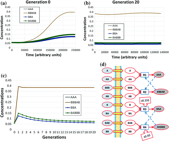

  

  As in Fig. 5.12, this figure shows the concentration versus. time (arbitrary units) of chemical species belonging to two independent sRAFs (d), during the lifespan of a single protocell (at the initial generation (a) and after 19 splits (b)), and during 20 generations at the division time (c). The two sRAFs have the same structure of Fig. 5.12, but all chemical species start from the same initial concentration; rather, the kinetic coefficients of the two reactions of the second sRAF are respectively diminished by a factor 3 and 2 (part (d) of the figure). Despite this gap, the finite membrane diffusion allows this second sRAF to reach a positive and stable configuration (part (c) of the figure—see (Villani et al. 2014) for more details)

Of course the validity of these properties depends on the values of the system parameters, but it holds for a wide range of values.⁴⁰ Remarkably the same properties are valid both for protocells where the relevant chemical reactions occur inside the whole system’s volume and for protocells where these reactions occur only in an internal spherical shell close to the surface (Villani et al. 2016, Calvanese et al. 2017).⁴¹

So we have shown that the particular form of resource limitation we are discussing—that is, a limitation on the rate of resource availability—significantly modifies the dynamics of growth of the chemical species in the protocell, which changes from exponential to sub-exponential. This change allows the survival within the same protocell of more sRAFs (not only to the fastest); therefore, protocells are able to host several different structures and therefore to simultaneously express various characteristics. Of course, this does not mean that slow sRAFs always survive: on the contrary, too slow sRAFs are normally lost.

5.6 A Comment on Evolvable Populations of Protocells

Protocells endowed with a Kauffman-type replicator dynamics are clearly a model where metabolic considerations play a central role. At the same time, however, the organization of the dynamic protocell components is also a form of information treatment and storage ; moreover, all these processes happen inside the same object (so information processing is “embodied”). One might therefore guess that protocells might represent entities sophisticated enough to constitute a valuable support for evolutionary processes.

Let us recall that, in order to undergo evolution, the individuals of a population should present the following characteristics (Lewontin 1970):

• 1. variation: the individuals should be somewhat different each other

• 2. reproduction : the individuals should be able to grow and produce descendants

  • a. the rates of growth and reproduction should depend on some characteristics of the individuals

• 3. heritability: there is a correlation between parents and offspring

While these properties are necessary, they may however be not sufficient for evolution to effective. In Chaps. 3 and 5 we presented a class of protocell models endowed with all these characteristics; in particular we highlighted some important bottlenecks that must be solved in order to allow protocells to undergo Darwinian evolution. We showed that once a coupling between the growth and fission rate of the container and that of the internal self-replicating molecules has been established, synchronization spontaneously emerges for a very wide range of dynamical hypotheses. Moreover, a protocell has the possibility to enhance and amplify (some) stochastic events that can spontaneously occur. New structures can be added to the ones already existing, other structures could change or even disappear. The particularly delicate aspect of successful changes (which should emerge but not necessarily replace the already existing characteristics) requires bounds on the growth rates, a constraint that the protocell membranes are able to effectively provide. In this way protocells are able to “remember” incremental improvements, an essential piece (Bedau and Packard 2003) toward evolvability (Wagner 2007).⁴² Besides these endogenous activities, protocells exchange energy and materials with their environment , and may react to the environmental changes by modifying their internal structure.

The autocatalytic properties of RAFs and their coupling with the protocell membrane guarantee the reproduction of the protocell materials; the same properties allow the offspring to grow and behave in a manner similar to that of their parents. The self-replicating molecules belonging to sRAFs are typically conserved in these processes and rule the protocell dynamics. New sRAFs could emerge, already existing sRAFs can change or even disappear. These changes are inherited by the protocell’s offspring. Because of this “central” and “ruling” role, the (self-replicating molecules belonging to) sRAFs are able to play the role of primitive inherited trait carriers—although acquiring or loosing entire groups of chemicals (those belonging to the sRAFs) is not a very flexible mechanism, as emphasised in Vasas et al. (2010). Anyway, protocells seem able to support evolutionary processes: “the real question is that of the organization of chemical networks . If … there can be in the same environment distinct, organizationally different, alternative autocatalytic cycles/networks, … then these can also compete with each other and undergo some Darwinian evolution” (Vasas et al. 2010).

Indeed, in last chapters we discussed an example of this organisation. A major difference between protocells as described in this book and actual living cells is the way information is stored and inherited: by using a useful classification (Hogeweg 2001) we can say that protocells show an attractor-based inheritance, whereas living cells show a storage-basedinheritance (clearly, with this assertion we are merely highlighting the fact that in the case of living cells a significant part of the information is stored in the static structure of specialised chemical compounds like DNA).⁴³

The quantity of storable information in attractor-based organisations depends on the number of their alternative stable states, which for protocells are determined by (the zone of) the chemistry where each individual is wandering. Noise , as discussed in this chapter, can also be very important, as it allows the population of protocells to perform an effective exploration of a significant part of the chemistry, and to reach areas where the protocells are able to growth and replicate and to increase the individuals’ complexity.

So different groups of protocells may reach different areas of their environment , or even may present different dynamical behaviours in the same zones. In this case the different groups of individuals can interact with each other, differently affecting the chemical composition of the local environment and in such a way giving birth to multiple levels of selection , an issue discussed in Hogeweg (2001). Indeed, local interactions among different individuals within a spatially extended environment could locally change it, leading to the formation of higher-level assemblies able to affect the behaviour of the single units composing them (Boerlijst and Hogeweg 1991a, b).

So, populations of protocells within spatially extended environments potentially could allow a very interesting flexibility and diversity.

On the other hand, the actual DNA -based living systems can store a lot of information at roughly equal energy/stability levels. The (not completely error-free) template-based DNA replication allow the inheritance of variations without requiring the acquisition or the loss of entire groups of chemicals; moreover, many of these mutations are not lethal, and a significant subset of them is even advantageous. Therefore, template-based systems are probably “more evolvable” (for a classification of long-term evolutionary dynamics, see also Bedau et al. 1998).

In any case, self-structuring objects may be a prerequisite to exploit stored information (Hogeweg 2001) and it would be very interesting to study the transition from attractor-based, limited inheritance to a storage-based , less limited form of inheritance (Vasas et al. 2010; Hogeweg 2001).

5.7 Appendix

We have introduced various models in Chaps. 4 and 5, describing their behaviours and explaining the reasons of our choices. In order to make it easier for the reader to clearly appreciate the value and limitations of these results, we summarize here the main features of these models.

They require the modelling of (i) the chemical reactions taking place in the system and (ii) the exchange properties of the system with the surrounding environment . Since we deal mainly with protocells, we will sometimes refer to this latter aspect as “the modelling of the container”.

The reactions happen inside the whole internal volume in CSTRs or in IRM protocell models, or only within a small fraction of this volume in NSRM protocell models⁴⁴; in all these cases we suppose that the internal environment is perfectly mixed. The exchange with the external environment is described as vanishing (in the case of a closed vessel) , as that of a CSTR , where there is a continuous inflow with constant concentration of solutes and an equal outflow or as a semipermeable membrane , or as that of a protocell, where the exchange of the chemical species that can pass through the semipermeable membrane is driven by their concentration gradient between the internal ad external chemical situation.

In Sect. 5.7.1 the chemical reaction system is described, while Sect. 5.7.2 is dedicated to the container properties. Finally, Sect. 5.7.3 briefly summarizes the protocell splitting process.

5.7.1 The Chemical Reaction System

As already discussed we make use of two kinds of reaction, cleavages and condensations:

$$ \begin{array}{*{20}l} {1.\,{\text{Cleavage}}\,AB + Z{\mathop{\longrightarrow}\limits^{{C_{Cl}}}}A + B + Z} \hfill \\ {2.\,{\text{Condensation}}{:}\,\left( {{\text{whole}}\,{\text{reaction}}{:}\,A + B + Z \to AB + Z} \right)} \hfill \\ {\quad \quad 1.\,{\text{Complex}}\,{\text{formation}}{:}\,A + Z{\mathop{\longrightarrow}\limits^{{C_{comp}}}}A:Z} \hfill \\ {\quad \quad 2.\,{\text{Complex}}\,{\text{dissociation}}{:}\,A:Z{\mathop{\longrightarrow}\limits^{{C_{diss}}}}A + Z} \hfill \\ {\quad \quad 3.\,{\text{Final}}\,{\text{condensation}}{:}\,A:Z + B{\mathop{\longrightarrow}\limits^{{C_{cond}}}}AB + Z} \hfill \\ \end{array} $$

(5.12)

where A and B stand for the substrates of the specific reaction, Z is the catalyst and A:Z is a transient complex. Since reactions that simultaneously involve three or more molecules are much rarer that bimolecular reactions, the condensation process is considered as composed of three steps: the first two create (reversibly) a temporary complex (composed by one of the two substrates and the catalyst) that can be used by a third reaction, which combines the complex and a second substrate to finally release the catalyst and final product.

If the concentrations of the various chemical species are high enough, the chemical reactions can be described by differential equations (ODEs), as usual in chemical kinetics , following the law of mass action . So, for each cleavage the concentration changes due to the cleavage reaction r that breaks chemical AB in chemicals A and B, under the action of catalyst Z is:

$$ \frac{d\left[ A \right]}{dt} = \frac{d\left[ B \right]}{dt} = - \frac{{d\left[ {AB} \right]}}{dt} = K_{cl} \left[ {AB} \right]\left[ Z \right] $$

(5.13)

where K _cl is the kinetic constant of the reaction r and square brackets denote volume concentrations.⁴⁵

Similarly, for each condensation d the concentration change of the chemicals A and B that condensate in chemical AB because of the presence of the catalyser Z, through the intermediate reactions involving the temporary chemical complex AB is:

$$ \left\{ {\begin{array}{*{20}l} {\frac{{d\left[ {AZ} \right]}}{dt} = K_{az}^{ + } \left[ A \right]\left[ Z \right] - K_{az}^{ - } \left[ {AZ} \right] - K_{bz} \left[ B \right]\left[ {AZ} \right]} \hfill \\ {\frac{d\left[ A \right]}{dt} = K_{az}^{ - } \left[ Z \right] - K_{az}^{ + } \left[ A \right]\left[ Z \right]} \hfill \\ {\frac{d\left[ B \right]}{dt} = - K_{bz} \left[ B \right]\left[ {AZ} \right]} \hfill \\ {\frac{d\left[ Z \right]}{dt} = K_{az}^{ - } \left[ {AZ} \right] - K_{az}^{ + } \left[ A \right]\left[ Z \right] + K_{bz} \left[ B \right]\left[ {AZ} \right]} \hfill \\ {\frac{{d\left[ {AB} \right]}}{dt} = K_{bz} \left[ B \right]\left[ {AZ} \right]} \hfill \\ \end{array} } \right. $$

(5.14)

K ⁺ _az , K ⁻ _az and K _bz are the kinetic constants of the complex formation, complex dissociation and complex condensation.⁴⁶ The overall concentration change of each chemical is of course the sum of all the changes due to the various reactions it partakes.

The ODEs can be numerically integrated. We typically use of an Euler method with step size control: in this case the integration with the container (modelled by ODEs) is straightforward.

If however the concentrations of some species are very low, randomness becomes significant and one has to resort to a truly stochastic approach , like the well-known one proposed by Gillespie (1976, 1977). In the case where the deterministic reaction rates were those of Eq. 5.14, the Gillespie reaction constants can be derived from the kinetic constant of Eq. 5.14 by means of the relations:

$$ \left\{ {\begin{array}{*{20}l} {C_{cl} = \frac{{K_{cl} }}{V}} \hfill \\ {C_{comp} = \frac{{K_{az}^{ + } }}{V}} \hfill \\ {C_{diss} = K_{az}^{ - } } \hfill \\ {C_{cond} = \frac{{K_{bz} }}{V}} \hfill \\ \end{array} } \right. $$

(5.15)

and the Gillespie algorithm can be applied:

• Step 0. (Initialization) Input the desired values for the M reaction constants c_l,…,c_M and the N initial molecular population numbers X₁,…,X_N. Set the time variable t and the reaction counter n both to zero. Initialize the uniform random number generator.

• Step 1. Calculate and store the M quantities α_l = h_lc_l,…, α_M = h_Mc_M for the current molecular population numbers, where h_ν is the product of the number of molecules of the substrates of the reaction R_ν. Also calculate and store as α₀ the sum of the M α_ν values (so that the quotient α_i/α approximates the occurrence probability of reaction i)

• Step 2. Calculate the time τ needed for the next reaction occur, and choose the index μ of the occurring reaction given the computed α _i values (see Gillespie 1976 for details)

• Step 3. Using the τ and μ values obtained in step 2, increase t by τ, and adjust the molecular population levels to reflect the occurrence of one R_μ reaction; e.g., if R_μ is a cleavage, then increase each product by 1 and decrease the substrate by 1. Then increase the reaction counter n by 1 and return to step 1.

In returning to step 1 from step 3, notice that it is necessary to recalculate only those quantities α_ν corresponding to reactions R_μ whose reactant population levels were just altered in step 3; also, α₀ may be recalculated simply by adding to α₀ the difference between each newly changed α_ν value and its corresponding old value. The schema is iterated until the desired time is reached.

5.7.2 The Exchange with the Environment

The chemical reaction system is contained within a vessel , which rules the interaction with the external environment. In the trivial case of a closed vessel the exchange with the external environment vanishes, so there is nothing else to add. In the cases of a CSTR and of a semipermeable membrane the exchange of chemicals is typically modelled using differential equations.

The CSTR involves a continuous inflow with constant concentration of solutes, while the outflow rates of the various chemicals are proportional to their concentrations in the reaction vessel. So, the differential equations ruling the exchange of each simulated chemical are:

$$ \frac{{d\left[ {x_{i} } \right]}}{dt} = J_{i} - \phi \left[ {x_{i} } \right]\quad i = 1, \ldots ,N $$

(5.16)

where J _i describes the intake of each chemical species (which may of course vanish) and ϕ represents the solution outflow rate. Of course, this is only the contribution to the total rate pf change that is due to transport.

In the case of vesicles and protocells with semipermeable membranes the external concentrations of the various chemical species are assumed to be constant (an approximation that is based on the hypotheses that the volume of the external environment is well-mixed and much larger than the internal volume—or the sum of the internal volumes if there are several vesicles). The transmembrane diffusion depends upon the features of the molecules but, as first ansatz, we simply assume that short molecules (namely those shorter than a threshold length L _perm ) can pass through the membrane while longer ones cannot.

So, in the case of extremely fast transmembrane diffusion , transport is assumed to be instantaneous, and the concentrations of the chemical species that can cross the membrane are assumed to be equal (and constant) on both sides, while the other molecules (i.e. those that are longer than L _perm ) are trapped inside the vesicle.

In the final part of Chap. 5 we analyse also the effects of a finite transmembrane diffusion rate. In this case the concentration of the short species are subject to the direct influence of the external environment, modelled by means of Fick’s law (Bird et al. 1976):

$$ \frac{{d\left[ {x_{i} } \right]}}{dt} = - \frac{{D_{i} S}}{h}\left( {\left[ {x_{i} } \right] - \xi_{i} } \right) $$

(5.17)

where [x _i ] and ξ _i are respectively the internal and the (constant) external concentrations of species i, D _i is its diffusion coefficient across the membrane with (constant) thickness h and surface area S (see also Sect. 5.2). Like in the case of instantaneous transport, molecules longer than L _perm never cross the membrane.

Moreover, some chemical species are coupled to the growth of the container . The models discussed in this book assume that these species act as specific catalysts for the production of membrane lipids, assuming abundant and buffered lipid precursors. Let C be the total number of lipid molecules (or moles) in the membrane . Then the equation for the growth rate of the container takes the form:

$$ \frac{dC}{dt} \cong \sum\limits_{i\,=\,1}^{N} {k_{i}^{cont} \left[ {x_{i} } \right]^{\gamma } V_{eff} } $$

(5.18)

where V _eff is the internal volume of the protocell where reactions occur and [x _i ] is the concentration of catalysts in the internal aqueous phase; the kinetic coefficients k _i are zero for all the species that do not contribute to the container growth. The kinetics of lipid formation are of order γ with respect to the concentration of catalyst, given the hypothesis of an infinite supply of lipid precursors inside the protocell. The lipids produced inside the protocell are assumed to be incorporated instantly into the membrane.

Protocells can grow and divide: during these processes their form and shape can change but, for reasons discussed in the text (see Sect. 3.5), we suppose that they are spherical with internal radius r _i with constant membrane width δ. So, in the case of IRM:

$$ V_{eff} \left( C \right) = V_{\text{int}} = \frac{1}{6\sqrt \pi }\left( {\frac{C}{\rho \delta }} \right)^{{\frac{3}{2}}} $$

(5.19)

where ρ represents the constant concentration of the lipids in the membrane.

If the reactions happen only within a distance ε from the inner surface of the membrane (as in NSRM models) we have:

$$ V_{eff} \left( C \right) = \frac{C}{\rho \delta }\varepsilon $$

(5.20)

Since the exchange with the environment is modelled by differential equations, its coupling with the internal reaction dynamics is straightforward when the latter is also described by ODEs, while it is less obvious in the case of the Gillespie approach.

Nevertheless, the Euler method that we use to integrate the equations describing the container dynamics can allow a simple merge of the two modules also in this second situation. Actually, the Euler schema implies that the variable changes are linked to a finite time interval: in our framework this time interval can be directly derived from the Gillespie algorithm , which therefore becomes the main systems’ engine. So the general schema is (see also Villani et al. 2014):

• While (simulation is non ended)

  • a. The Gillespie framework holds, and computes a finite time interval Δt_g

  • b. The simulation time is updated t _s  = t _s  + Δt _g

  • c. For each chemical x _i

    • i. the time passed from the chemical last change is updated LC _i  = LC _i  + Δt _g

    • ii. its flows through the container is updated fw _i  = fw _i  + f(rules, LC _i )

    • iii. if |int(fw _i )-fw _i | ≥ 1, the number of molecules of x _i is varied of int(fw _i ), fw _i is decremented by int(fw _i ) and LC _i is set to 0

Int(X) and f(rules, LC _i ) indicate respectively the integer part of X and the dynamical rules (derived from of the differential equations description) that drive the chemical i mass exchange with the external environment through the membrane. The time interval Δt_g is very tiny (it correspond to the formation/disappearance of few molecules) and is therefore compatible with the Euler schema used for the container’s module.⁴⁷

By the way, note that if the volume is time dependent and if the process is quasi-static (the volume variation is not too fast) it is possible to simulate by a Gillespie-like method also systems where the container volume can vary in time (it is enough to take into consideration the volume changes and recalculate the Gillespie reaction constants during the simulation—see Carletti and Filisetti 2012 for further details).

5.7.3 The Protocell Splitting Process

In the case of growing and dividing protocell we have to model the growth stop and the successive splitting phase.

As discussed in detail in Sects. 3.2 and 5.1, it assumed that the vesicle splits into two approximately equal parts when a certain threshold value θ of the container surface or mass is reached. So, at each splitting event the number of molecules of the container C and the number of molecules of the chemical species x _i change in time following the simple rule:

$$ \left\{ {\begin{array}{*{20}l} {C\left( {t + 1} \right) = \frac{C\left( t \right)}{2}} \hfill \\ {x_{i} \left( {t + 1} \right) = \zeta x_{i} \left( t \right)} \hfill \\ \end{array} } \right. $$

(5.21)

where t and t + 1 are the times of two consecutive splitting events and ζ takes the value 0.5 if there is no material loss during splitting, or ≈0.354 in case of loss of materials—see Sect. 5.1.