Chemical Risk Characterization

Abstract

Fundamentally, risk characterization consists of estimating the probable incidence of adverse impacts to potential receptors, under the various exposure conditions associated with a chemical hazard situation. It involves an integration of the hazard effects and exposure assessments—in order to arrive at an estimate of the health risk to the exposed population. In general, all information derived from each step of a chemical exposure-cum-hazard assessment are integrated and utilized during the risk characterization—so as to help project the degree and severity of adverse health effects in the populations potentially at risk.

Fundamentally, risk characterization consists of estimating the probable incidence of adverse impacts to potential receptors , under the various exposure conditions associated with a chemical hazard situation. It involves an integration of the hazard effects and exposure assessments—in order to arrive at an estimate of the health risk to the exposed population. In general, all information derived from each step of a chemical exposure-cum-hazard assessment are integrated and utilized during the risk characterization—so as to help project the degree and severity of adverse health effects in the populations potentially at risk.

Risk characterization is indeed the final step in the risk assessment process, and this also becomes the first input into risk management programs . Thus, risk characterization serves as a bridge between risk assessment and risk management—making it a key factor in the ultimate decision-making process that would often be undertaken to help address chemical exposure problems. Classically, risk characterization commonly will entail a statement regarding the ‘response’ or ‘risk of harm’ that is expected in the population under an associated set of exposure conditions, together with a description of uncertainties (NRC 1983). Through probabilistic modeling and analyses, uncertainties associated with the risk evaluation process can be assessed properly, and their effects on a given decision accounted for systematically. In this manner, the risks associated with given decisions may be delineated—and then appropriate corrective measures taken accordingly. This chapter elaborates the mechanics of the risk characterization process, together with example risk presentation modalities that would tend to, among several other things, facilitate effective risk management and/or risk communication efforts.

1 Fundamental Issues and Considerations Affecting the Risk Characterization Process

The chemical risk characterization process generally consists of an integration of the toxicity and exposure assessments —resulting in a quantitative estimation of the actual and potential risks and/or hazards associated with a chemical exposure problem. Broadly stated, risk from human exposure to chemicals is a function of dose or intake and potency, viz.:

$$ Risk\ from\ chemical\kern0.28em exposure=\left[ Dose\ of\ chemical\right]\times \left[ Chemical\ potency\right] $$

(11.1)

Overall, chemical risk characterization is viewed as a process by which dose-response information is integrated with quantitative estimates of human exposure derived in an exposure assessment; the result is a quantitative estimate of the likelihood that humans will experience some form of adverse health effects under a given set of exposure assumptions. During the risk characterization, chemical-specific toxicity information is traditionally compared against both field measured and estimated chemical exposure levels (and in some cases, those levels predicted through fate and behavior modeling) in order to determine whether concentrations associated with a chemical exposure problem are of significant concern. In principle, the process should also consider the possible additive or cumulative and related effects of exposure to mixtures of the chemicals of potential concern.

Two general types of health risk are typically characterized for each potential exposure pathway considered—viz.: potential carcinogenic risk, and potential noncarcinogenic hazard. Broadly speaking, characterization of the potential health effects of potential carcinogenic versus noncarcinogenic chemicals are approached very differently. A key difference in the approaches arises from the conservative assumption that substances with possible carcinogenic action typically behave via a no-threshold mechanism, whereas other toxic actions may have a threshold (i.e., a dose below which few individuals would be expected to show a response of concern)—albeit this viewpoint has been challenged, and remains in debate. Thus, under the no-threshold assumption, it becomes necessary to calculate a risk number—whereas for chemicals with a threshold, it is possible to simply characterize an exposure as above or below the designated threshold level (generally termed a reference dose or reference concentration). Also, potential carcinogenic risk is evaluated by averaging exposure over a ‘normal’ human lifetime, whereas potential noncarcinogenic hazard is evaluated by averaging exposure over the total exposure period considered in practice. Indeed, depending on the nature of populations potentially at risk from a chemical exposure problem, different types of risk metrics or parameters may be employed in the risk characterization process. At any rate, the cancer risk estimates and hazard quotient-cum-hazard index estimates are the measures of choice typically used to define potential risks to human health [see Sects. 11.2 and 11.3]. Indeed, it is almost indispensable to have these measures available to support effectual public health risk management programs. Consequently, the health risks to potentially exposed populations resulting from chemical exposures are characterized through a calculation of non-carcinogenic hazard quotients/indices and/or carcinogenic risks (CAPCOA 1990; CDHS 1986; USEPA 1986a, 1989a).

In the final analysis, an effective risk characterization should be carried out in such a manner that it fully, openly, and clearly characterize risks as well as disclose the scientific analyses, uncertainties, assumptions, and science policies that underlie decisions utilized throughout the risk assessment and risk management processes. In fact, every risk assessment should clearly delineate the strengths and weaknesses of the data, the assumptions made, the uncertainties in the methodology, and the rationale used in reaching the conclusions (e.g., similar or different routes of exposure, and metabolic differences between humans and test animals). Furthermore, the hazard and risk assessment of human exposure to chemicals must take a miscellany of other critical issues into account—especially as relates to scenarios whereby chemical interactions may significantly influence toxic outcomes; chemical interactions are indeed very important determinants in evaluating the potential hazards and risks of exposure to chemical mixtures (Safe 1998).

Lastly, it is noteworthy that, a health risk assessment/characterization is only as good as its component parts—i.e., the hazard characterization, the dose-response analysis, and the exposure assessment. Confidence in the results of a risk assessment is thus a function of the confidence in the results of the analysis of these distinct key elements, and indeed their corresponding ingredients. In the end, several important issues usually will have very significant bearing on the processes involved in completing risk characterization tasks designed to support effective public health risk management programs; a number of the particularly important topics/issues are discussed below.

1.1 Corrections for ‘Non-standard’ Population Groups

During the risk estimation, the exposure information is customarily combined with dose-response information. In the processes involved, care must be taken to ensure that the assumptions about population parameters in the dose-response analysis are consistent with the population parameters used in the exposure analysis; common procedures for assuring such consistency is provided in the literature elsewhere (e.g., USEPA 1997a, b, c, d, e, f, g, h; West et al. 1997). In general, when the population of interest is different in comparison with the ‘standard’ population assumed in the dose-response assessments, then the dose-response parameter may need to be adjusted accordingly. Furthermore, when the population of interest is different from the population from which the often-used default exposure factors were derived, then the exposure factor may also need to be adjusted accordingly. A good example of a ‘non-standard’ sub-population would be a sedentary hospital population with lower than 20 m³/day air intake rates (as is often assumed for most ‘standard’ population groups). Also, an example of such a sub-population relates to mean body weight (that is different from the often assumed standard of 70 kg); for instance, under some circumstances, females usually may be assumed to have an average body weight of 60 kg, and also children’s body weights will be dependent on their age.

To exemplify the requisite procedures for modifying standard parameters for non-standard populations, consider a recommended value for the average consumption of tap water by adults in a population group to be 1.4 L/day. Assume the drinking water unit risk for chemical X is 8.3 × 10⁻⁶ per μg/L, and that this was calculated from the slope factor assuming the standard intake, I_ws, of 2 L/day. Then, for the population group drinking 1.4 L of tap water per day, the corrected drinking water unit risk should be (USEPA 1997a, b, c, d, e, f, g, h):

$$ \left[8.3\times {10}^{-6}\right]\times \left[\frac{1.4}{2}\right]=5.8\times {10}^{-6}\;\mathrm{per}\;\upmu \mathrm{g}/\mathrm{L} $$

Subsequently, the risk to the average individual can then be estimated by multiplying this value by the average concentration (in units of μg/L).

Another illustrative example using the procedures provided by the US EPA (USEPA 1997a, b, c, d, e, f, g, h) involves estimating the risk specifically for women drinking the water contaminated with chemical X. Now, if the body weight, W^p, of the population of interest differs from the body weight, W^s, of the population from which the standard exposure values were derived, then a modeling adjustment may have to be made in estimating the intake of food, water, and air in this population (USEPA 1997a, b, c, d, e, f, g, h; West et al. 1997). If it is assumed that this group of women has an average body weight of 60 kg, then the correction factor for the drinking water unit risk (disregarding the correction discussed above with respect to consumption rate) is:

$$ {\left[\frac{70}{60}\right]}^{2/3}=1.11 $$

Thus, the corrected water unit risk for chemical X is:

$$ \left[8.3\times {10}^{-6}\right]\times \left[1.11\right]=9.2\times {10}^{-6}\;\mathrm{per}\;\upmu \mathrm{g}/\mathrm{L} $$

As indicated previously, the risk to the average individual is subsequently estimated by multiplying this value by the water concentration.

1.2 Adjustments for Chemical Absorption: Administered vs. Absorbed Dose

Oftentimes, absorption adjustments may become necessary during the risk estimation process—in order to ensure that the exposure estimate and the toxicity value being compared during the risk characterization are both expressed as absorbed doses, or both expressed as administered doses (i.e., intakes). Adjustments may also be required for different vehicles of exposure (e.g., water, food, or soil)—albeit, in most cases, the unadjusted toxicity value will provide a reasonable or conservative estimate of risk. Furthermore, adjustments may be needed for different absorption efficiencies, depending on the medium of exposure; in general, correction for fractional absorption is particularly appropriate when interaction with environmental media or other chemicals may alter absorption from what would typically be expected for the pure compound. Correction may also be necessary when assessment of exposure is via a different route of contact than what was utilized in the experimental studies used to establish the toxicity parameters (i.e., the SFs, RfDs, etc. discussed in Chap. 10). For instance, only limited toxicity reference values generally exist for dermal exposure; consequently, oral values are frequently used to assess risks from dermal exposures (USEPA 1989d). On the other hand, most RfDs and some carcinogenic SFs usually are expressed as the amount of substance administered per unit time and unit body weight, whereas exposure estimates for the dermal route of exposure are eventually expressed as absorbed doses. Thus, for dermal exposures, it may become particularly important to adjust an oral toxicity value from an administered to an absorbed dose—generally carried out as indicated below (USEPA 1989d).

• Adjustment of an ‘administered dose’ to an ‘absorbed dose’ for RfDs. The ‘administered dose’-based RfD (RfD_adm) of a chemical with oral absorption efficiency, ABS, in the species on which the RfD is based may be adjusted to an ‘absorbed dose’-based RfD (RfD_abs); this is achieved by simply multiplying the unadjusted RfD by the absorption efficiency percent—as follows:

$$ {\mathrm{RfD}}_{\mathrm{abs}}={\mathrm{RfD}}_{\mathrm{adm}}\times \mathrm{ABS} $$

(11.2)

This can then be compared with the amount estimated to be absorbed dermally.

• Adjustment of an ‘administered dose’ to an ‘absorbed dose’ for SFs. The ‘administered dose’-based SF (SF_adm) of a chemical with oral absorption efficiency, ABS, in the species on which the SF is based may be adjusted to an ‘absorbed dose’-based SF (SF_abs); this is achieved by simply dividing the unadjusted SF by the absorption efficiency percent—as follows:

$$ {\mathrm{SF}}_{\mathrm{abs}}=\frac{{\mathrm{SF}}_{\mathrm{adm}}}{\mathrm{ABS}} $$

(11.3)

This can then be used to estimat e the cancer risk associated with the estimated absorbed dose for the dermal route of exposure.

• Adjustment of an exposure estimate to an absorbed dose. If the toxicity value is expressed as an absorbed rather than an administered dose, then it may become necessary to convert the exposure estimate from an intake into an absorbed dose for comparability. The unadjusted exposure estimate or intake (CDI_adm) of a chemical with absorption efficiency, ABS, may be converted to an ‘adjusted exposure’ or absorbed dose (CDI_abs); this is achieved by simply multiplying the unadjusted CDI by the absorption efficiency percent—as follows:

$$ {\mathrm{CDI}}_{\mathrm{abs}}={\mathrm{CDI}}_{\mathrm{adm}}\times \mathrm{ABS} $$

(11.4)

This can then be used in comparisons with the RfD or SF that has been developed based on an absorbed (not administered) dose.

Absorption efficiency adjustment procedures are elaborated further elsewhere in the literature (e.g., USEPA 1989d, 1992a, b, c, d, e). Meanwhile, it is noteworthy that, for evaluations of the dermal exposure pathway, if the oral toxicity value is already expressed as an absorbed dose, then it is not necessary to adjust the toxicity value. Also, exposure estimates should not be adjusted for absorption efficiency if the toxicity values are based on administered dose. Furthermore, in the absence of reliable information, 100% absorption is usually used for most chemicals; for metals, an approximately 10% absorption may be considered a reasonable upper-bound for other than the inhalation exposure route.

In general, absorption factors should not be used to modify exposure estimates in those cases where absorption is inherently factored into the toxicity/risk parameters used for the risk characterization. Thus, ‘correction’ for fractional absorption is appropriate only for those values derived from experimental studies based on absorbed dose. In other words, absorbed dose should be used in risk characterization only if the applicable toxicity parameter (e.g., SF or RfD) has been adjusted for absorption; otherwise, intake (unadjusted for absorption) are used for the calculation of risk levels.

1.3 Aggregate Effects of Chemical Mixtures and Multiple Exposures

Oftentimes in the study of human exposures to chemical hazards, it becomes necessary to carry out aggregate and cumulative exposure and risk assessments. In fact, in most situations, it is quite important to consider both aggregate and cumulative exposures—to facilitate the making of effectual risk assessment and risk management decisions, as well as help the process of setting chemical tolerance or safe levels for human exposures. In general, aggregate exposures may occur across different pathways and media that contribute to one or more routes of an individual receptor’s exposure—which then becomes the basis for determining cumulative risks.

Cumulative risk refers to effects from chemicals that have a common mode of toxicological action—and thus have aggregate exposure considerations as part of the assessment process (Clayton et al. 2002). Indeed, whereas some chemical hazard situations involve significant exposure to only a single compound, most instances of chemical exposure problems can involve concurrent or sequential exposures to a mixture of compounds that may induce similar or dissimilar effects over exposure periods ranging from short-term to a lifetime (USEPA 1984a, 1986b). Meanwhile, it is notable that evaluating mixtures of chemicals is one of the areas of risk assessment with obviously many uncertainties; this is especially so, because several types of interactions in chemical mixtures are possible—including the following key distinct attributes :

• Additive—wherein the effects of the mixture equals that of adding the effects of the individual constituents.

• Synergistic—wherein the effects of the mixture is greater than obtained by adding the effects of the individual constituents.

• Antagonistic—wherein the effects of the mixture is less than obtained by adding the effects of the individual constituents.

Of particular concern are those mixtures where the effects are synergistic. Unfortunately, the toxicology of complex mixtures is not very well understood—complicating the problem involved in the assessment of the potential for these compounds to cause various health effects. Nonetheless, there is the need to assess the cumulative health risks for the chemical mixtures, despite potential large uncertainties that may exist. The risk assessment process must, therefore, address the multiple endpoints or effects, and also the uncertainties in the dose-response functions for each effect.

Finally, in combining multi-chemical risk estimates for multiple chemical sources, it should be noted here that, if two sources do not affect the same individual or subpopulation, then the sources’ individual risk estimates (and/or hazard indices) do not quite influence each other—and, therefore, these risks should not be combined. Thus, one should not automatically sum risks from all sources evaluated for a chemical exposure problem—i.e., unless if it has been determined/established that such aggregation is appropriate. On the other hand, potential receptors are typically exposed not to isolated chemical sources, but rather to a complex, dilute mixture of many origins. Considering how many chemicals are present in the wide array of consumer products, and in the human environments, there are virtually infinite number of combinations that could constitute potential synergisms and antagonisms . In the absence of any concrete evidence of what the interactive effects might be, however, an additive method that simply sums individual chemical effects on a target organ is usually employed in the evaluation of chemical mixtures.

1.3.1 Carcinogenic Chemical Effects

The common method of approach in the assessment of chemical mixtures assumes additivity of effects for carcinogens when evaluating multiple carcinogens—albeit alternative procedures that are more realistic and/or less conservative have been proposed for certain situations by some investigators (e.g., Bogen 1994; Chen et al. 1990; Gaylor and Chen 1996; Kodell and Chen 1994; Slob 1994). In any case, prior to a summation for aggregate risks, estimated cancer risks should perhaps be (preferably) segregated by weight-of-evidence (or strength-of-evidence) category for the chemicals of concern—the goal being to provide a clear understanding of the risk contribution of each category of carcinogen.

1.3.2 Systemic (Non-cancer) Chemical Effects

For multiple chemical exposures to non-carcinogens and the non-carcinogenic effects of carcinogens, constituents should be grouped by the same mode of toxicological action (i.e., those that induce the same physiologic endpoint—such as liver or kidney toxicity). Cumulative non-carcinogenic risk is evaluated through the use of a hazard index that is generated for each health or physiologic ‘endpoint’. Physiologic/toxicological endpoints that will normally be considered with respect to chronic toxicity include: cardiovascular systems (CVS); central nervous system (CNS); gastrointestinal (GI) system; immune system; reproductive system (including teratogenic and developmental effects); kidney (i.e., renal); liver (i.e., hepatic); and the respiratory system.

In fact, in a strict sense, constituents should not be grouped together unless they induce/affect the same toxicological/physiologic endpoint. Thus, in a well-defined risk characterization exercise, it becomes necessary to segregate chemicals by organ-specific toxicity—since strict additivity without consideration for target-organ toxicities could over-estimate potential hazards (USEPA 1986b, 1989d). Accordingly, the ‘true’ hazard index is preferably calculated only after putting chemicals into groups with same physiologic endpoints. Listings of chemicals with their associated non-carcinogenic toxic effects on specific target organ/system can be found in such databases as IRIS (Integrated Risk Information System), as well as in the literature elsewhere (e.g., Cohrssen and Covello 1989a; USEPA 1996a, b, c, d, e, f).

1.4 Updating the Inhalation Exposure/Risk Paradigm

Traditionally, the inhalation exposure route has been evaluated by using the ‘inhalation RfD’ (expressed in units of mg/kg day) and the ‘inhalation SF’ (expressed in units of [mg/kg day]⁻¹) [see Chap. 10], integrated with the estimated intake values (generally expressed in units of mg/kg day) [see Chap. 9], to arrive at probable risk estimates. However, recent works call for variant approaches for determining exposure and risk from inhaled chemicals—especially in order for it to be consistent with inhalation dosimetry methodologies currently used by a number of institutions/agencies (such as the US EPA). Generally speaking, the ‘inhalation dosimetry methodology’ describes a refined recommended approach for interpreting inhalation toxicity studies in laboratory animals, or studies of occupational exposures of humans to airborne chemicals; under this approach, the experimental exposures are typically extrapolated to a ‘human equivalent concentration’ (HEC)—and a ‘reference concentration’ (RfC) is typically calculated by dividing the HEC by appropriate uncertainty factors (UFs) [see Chap. 10]. The HEC, developed in accordance with the inhalation dosimetry methodology, typically is also used in developing an ‘inhalation unit risk’ (IUR) for cancer risk assessment (which may also be called an inhalation cancer slope factor) [see Chap. 10]. Ultimately, the procedure is used to calculate published RfCs and IURs—such as documented in USEPA’s IRIS profiles, and indeed other similar toxicological reference documents, etc.

Under this new paradigm noted here, it is generally recommended that when estimating risk via inhalation, risk assessors/analysts should use the concentration of the chemical in air as the exposure metric (e.g., mg/m³ or μg/m³)—i.e., rather than a use of inhalation intake of a contaminant in air based on IR and BW (e.g., mg/kg day). In this case, some of the intake equations described in Chap. 9 may not quite be wholly consistent with the principles of the inhalation dosimetry methodology—especially because the amount of the chemical that reaches the target site is not a simple function of IR and BW; instead, the interaction of the inhaled contaminant with the respiratory tract is affected by factors such as species-specific relationships of exposure concentrations (ECs) to deposited/delivered doses and physiochemical characteristics of the inhaled contaminant. The inhalation dosimetry methodology also considers the target site where the toxic effect occurs (e.g., the respiratory tract or a location in the body remote from the portal-of-entry) when applying dosimetric adjustments to experimental concentrations (USEPA 1994a, b, c, d, e, f, g).

In the end, it becomes necessary to appropriately characterize exposures in a manner that is consistent with the inhalation dosimetry methodology. The general approach involves the estimation of exposure concentrations (ECs) for each receptor exposed to contaminants via inhalation in the risk assessment; ECs are time-weighted average concentrations derived from measured or modeled contaminant concentrations in air at a locale or within an ‘exposure object’—and possibly further adjusted based on the characteristics of the exposure scenario being evaluated. Representative equations for estimating ECs are presented below—with the ECs typically provided in units of μg/m³.

1.4.1 Estimating Exposure Concentrations for Use in Cancer Risk Assessments

The estimation of an EC when assessing cancer risks characterized by an IUR encompasses a contaminant concentration in air (CA) measured at an exposure point, and at an appropriate locale or within an ‘exposure target’, as well as scenario-specific parameters (such as the exposure duration and frequency); the ECs are typically based on either estimated (i.e., modeled) or measured contaminant concentrations in air. Ultimately, the EC characteristically takes the form of a CA that is time-weighted over the duration of exposure, and incorporates information on activity patterns for the specific locale and/or further utilizes professional judgment as part of the overall process.

The general equation for estimating an EC for use with an IUR would be as follows (USEPA 2009):

$$ \mathrm{EC}\kern0.5em \left(\upmu \mathrm{g}/{\mathrm{m}}^3\right)=\frac{\left[ CA\times ET\times EF\times ED\right]}{AT} $$

(11.5)

where: EC (μg/m³) = exposure concentration; CA (μg/m³) = contaminant concentration in air; ET (h/day) = exposure time; EF (days/year) = exposure frequency; ED (years) = exposure duration; and AT (lifetime in years × 365 days/year × 24 h/day) = averaging time (viz., lifetime in years × 365 days/year × 24 h/day).

1.4.2 Estimating Exposure Concentrations for Use in Non-cancer Risk Assessments

When estimating ECs for non-cancer or hazard effects characterized by a use of the RfC, varying EC equations would typically be used based on the scenario duration and frequency of exposure; overall, the following general equations would typically be utilized for estimating an EC for use with an RfC (USEPA 2009):

$$ \mathrm{EC}\kern0.5em \left(\upmu \mathrm{g}/{\mathrm{m}}^3\right)= CA $$

(11.6a)

where: EC (μg/m³) = exposure concentration; CA (μg/m³) = contaminant concentration in air.

$$ \mathrm{EC}\kern0.5em \left(\upmu \mathrm{g}/{\mathrm{m}}^3\right)=\frac{\left[ CA\times ET\times EF\times ED\right]}{AT} $$

(11.6b)

where: EC (μg/m³) = exposure concentration; CA (μg/m³) = contaminant concentration in air; ET (h/day) = exposure time; EF (days/year) = exposure frequency; ED (years) = exposure duration; and AT (ED in years × 365 days/year × 24 h/day) = averaging time (viz., ED in years × 365 days/year × 24 h/day). It is notable that, if the duration of the exposure period is less than 1 year, the units in the above equation can be changed to the following: EF (days/week); ED (weeks/exposure period); and AT (hour/exposure period).

First, it is important to assess the duration of the exposure scenario at a locale or within a ‘exposure target’; invariably, the decision has to be made as to whether the duration of the exposure scenario is generally acute, subchronic, or chronic—recognizing that effects from a single or short-term exposure can differ markedly from effects resulting from repeated exposures. The response by the exposed person depends upon factors such as whether the chemical accumulates in the body, whether it overwhelms the body’s mechanisms of detoxification or elimination, or whether it produces irreversible effects (Eaton and Klaassen 2001). Thus, ideally, the chemical-specific elements of metabolism and kinetics, reversibility of effects, and recovery time should be considered as part of this recommended process when defining the duration of a site-specific exposure scenario (USEPA 2009).

Next is the assessment of the exposure pattern for each exposure scenario at a site or locale; this generally entails comparing the exposure time and frequency for the subject case to that of a typical subchronic or chronic toxicity test (USEPA 2009).

The final step would consist of estimating the EC for the specific exposure scenario based on the preceding decisions. For each acute exposure period at a locale, the EC is equal to the CA—estimated by using Eq. (11.6a) provided above; by the way, exposure periods with significantly less frequency should be treated as acute exposures. For longer-term exposures, the exposure time, frequency, and duration for each receptor being evaluated as well as the period over which the exposure is averaged (i.e., the averaging time (AT)) to arrive at a time-weighted EC should be taken into consideration; thus, if there are one or more exposure periods that are generally as frequent as a subchronic toxicity test, Eq. (11.6b) should be used to estimate a subchronic EC for each of these exposure periods. If the exposure pattern is generally as frequent as a chronic toxicity test of an occupational study, Eq. (11.6b) should be used to estimate a single chronic EC for the duration of the exposure.

Ultimately, it is important to use the EC equation that most closely matches the exposure pattern and duration in relation to the problem on hand. For instance, if the exposure pattern for a given problem scenario consists of a series of short (e.g., 4-h) periods of high exposure separated by several days of no exposure, then perhaps estimating an acute EC for each acute exposure period might be the most appropriate modality to adopt. On the other hand, if the chronic EC equation (viz., Eq. (11.6b)) were to be used instead, then the result would be an average EC value that may lead to an underestimation of the risk since the inhaled concentrations could be higher than acute toxicity values during periods of exposure .

1.4.3 Estimating Exposure Concentrations in Multiple Microenvironments

When detailed information on the activity patterns of a receptor at a locale is available, risk assessors/analysts can use these data to estimate the EC for either non-carcinogenic or carcinogenic effects arising from a problem situation. The activity pattern data generally describe how much time a receptor spends, on average, in different microenvironments (MEs)—each of which may have a different contaminant concentration level; a microenvironment may be defined as a delineated space that can be treated as a well-characterized, relatively homogeneous location with respect to pollutant concentration for a specified time period (e.g., rooms in homes, restaurants, schools, offices, inside vehicles, or outdoors) (USEPA 2004a, b, c, d, e, f, g). By combining data on the contaminant concentration level in each ME and the activity pattern data, the risk assessor can calculate a time-weighted average EC for a receptor. Meanwhile, because activity patterns (and hence, MEs) can vary over a receptor’s lifetime, it is generally recommended that risk assessors pursuing the ME approach first calculate a time-weighted average EC for each exposure period characterized by a specific activity pattern (e.g., separate ECs for a school-aged child resident and a working adult resident); these exposure period-specific ECs can then be combined into a longer term or lifetime average EC by weighting the EC by the duration of each exposure period (USEPA 2004a, b, c, d, e, f, g).

Overall, the ME approach can be used to estimate an average EC for a particular/specific exposure period during which a receptor has a specified activity pattern. As a simplified example, consider the case of a residential receptor that may be exposed to a higher concentration of a contaminant in air in the bathroom for 30 min/day while showering, and then exposed to a lower concentration in the rest of the house for the remaining 23.5 h/day. In such cases, the CA value experienced in each ME weighted by the amount of time spent in each ME may be used to estimate an average EC for the period of residency in that house—using the following equation (USEPA 2004a, b, c, d, e, f, g, 2009):

$$ {\mathrm{EC}}_{\mathrm{j}}\kern0.5em \left(\upmu \mathrm{g}/{\mathrm{m}}^3\right)=\sum_{i=1}^n\left({CA}_i\times {ET}_i\times {EF}_i\right)\times \frac{ED_j}{AT_j} $$

(11.7a)

where: EC_j (μg/m³) = average exposure concentration for exposure period j; CA_i (μg/m³) = contaminant concentration in air in ME i; ET_i (h/day) = exposure time spent in ME i; EF_i (days/year) = exposure frequency for ME i; ED_j (years) = exposure duration for exposure period j; and AT_j (h) = averaging time = ED_j × 24 h/day × 365 days/year. It is noteworthy here that, if one or more MEs involve acute exposures, then a supplemental analysis should probably be carried out—comparing the CA for each of those MEs to a corresponding acute toxicity value, to ensure that receptors are protected from potential acute health effects. Indeed, this approach may also be used to address exposures to contaminants in outdoor and indoor environments at locations where both indoor and outdoor samples have been collected or where the vapor intrusion pathway has been characterized.

Furthermore, the ME approach may be used in estimating an average exposure concentration across multiple exposure periods. To derive an average EC for a receptor over multiple exposure periods, the average EC from each period (as calculated above in Eq. (11.7a)) can be weighted by the fraction of the total exposure time that each period represents, using the following equation (USEPA 2004a, b, c, d, e, f, g, 2009):

$$ \mathrm{ECLT}\kern0.5em \left(\upmu \mathrm{g}/{\mathrm{m}}^3\right)=\frac{\sum \left({EC}_j\times {ED}_j\right)}{AT_j} $$

(11.7b)

where: ECLT (μg/m³) = long-term average exposure concentration; EC_j (μg/m³) = average exposure concentration of a contaminant in air for exposure period j; ED_j (years) = duration of exposure period j; and AT (years) = averaging time. For example, when estimating cancer risks, the risk assessor may calculate a lifetime average EC where the weights of the individual exposure periods are the duration of the period, ED_j, divided by the total lifetime of the receptor. Alternatively, when estimating an HQ, risk assessors/analysts can use Eq. (11.7b) to calculate less-than-lifetime average ECs across multiple exposure periods; in that case, the AT will equal the sum of the individual EDs for all of the exposure periods. Once again it is worth the mention here that when evaluating cancer risk, the AT is equal to lifetime in years, and when evaluating non-cancer hazard, the AT is equal to the sum of the EDs for each exposure period .

1.5 Fundamental Considerations in the Health Assessment of Carcinogens

Cancer risk assessment by necessity involves a number of assumptions—most of which reflect scientific and policy judgments . In general, in the absence of data to the contrary, a substance that has been shown to cause cancer in animals is presumed to pose a potential carcinogenic risk to humans. However, as more knowledge on particular agents and the oncogenic process in general becomes available, the position on these issues becomes subject to change. A number of fundamental but critical issues affecting the health risk assessment of carcinogens are enumerated below.

1.5.1 Qualitative Issues

Several qualitative issues affect the health assessment of carcinogens—most importantly, the topics identified below (IARC 1987; NTP 1991; USEPA 1986a, b, c, d, e, f).

• ‘Weight/Strength of Evidence’ . A ‘weight-of-evidence’ or a ‘strength-of-evidence’ approach may be adopted in evaluating all the relevant case data available on a given carcinogenic chemical. The general types of evidence that may be used for qualitatively identifying carcinogens include: case studies, epidemiological studies, long-term animal bioassays, short-term tests, and structure-activity relationships. Specific factors that are typically evaluated in determining if a substance poses a carcinogenic risk to humans include, but are not limited to: the quality of the toxicity studies (namely, relating to the choice of appropriate control groups; sufficient number of animals; administration route; dose selection; tumor types; etc.), and the relevance of animal data to humans. Ultimately, a narrative statement may be used to incorporate the weight/strength-of-evidence conclusions—i.e., in lieu of alphanumeric designations alone being used to convey qualitative conclusions regarding the chemical carcinogenicity.

• Mechanistic Inference and Species Concordance . Carcinogenesis is generally viewed as a multistage process—proceeding from initiation, through promotion, and progression. Carcinogens may work through mechanisms that directly or indirectly affect the genome. Commonly, it is assumed that many or most carcinogens are characterized by the absence of a threshold in eliciting a tumorigenic response. On the other hand, the presence or absence of a threshold for one step in the multistage process of carcinogenesis does not necessarily imply the presence or absence of a threshold for other steps, or the entire process. For example, carcinogenic effects of some agents may result from non-physiological responses to the agents, such as extensive organ damage; under such circumstances, the relevance of the animal data to humans should be evaluated on a case-by-case basis—with a view towards extending its assessment effort beyond the dominant paradigm of carcinogenesis (i.e., initiation, promotion, and progression).

• Exposure Route Specificity . In the analysis of potential carcinogenic risk of chemical agents to humans, it is generally important to address the issue of exposure route specificity. In fact, for some agents, exposure might result in adverse health effects via one route only; for example, whereas chronic oral exposures to an agent may not result in cancer in animals and/or humans, the same agent may be carcinogenic via inhalation in the same species. Accordingly, the potential health risk of toxic substances should be evaluated by carefully taking into account the relevant route(s) of exposure. In the absence of data to the contrary, however, an agent that is carcinogenic via one route may be considered to be a potential carcinogen via alternate routes as well.

• Role of Epidemiological Data . Epidemiological studies generally provide direct information on the carcinogenic risk of chemical agents to humans. For this reason, in evaluating the potential human cancer risks, a higher weight may be assigned to well-designed and well-executed epidemiological studies than to animal studies of comparable quality. Even so, the observational nature of such studies, as well as the use of indirect measures of exposure, can sometimes constrain the overall interpretation of the data. In any case, it is noteworthy that, although an agent may not have been shown to be a carcinogen in a well-designed epidemiological study, a potential association between exposure to the agent and human cancer cannot be completely ruled out. Indeed, the potential for an association will remain—especially if relevant animal data suggest that a carcinogenic effect exist; this premise would also apply in the case of health effects other than cancer.

On the whole, descriptive epidemiological studies may be useful in generating/refining hypotheses that suggest further in-depth studies. These studies also provide limited information on causal relationships. Alternatively, analytical epidemiological investigations, such as case-control or cohort studies, can provide the basis for testing causal associations—and these are an invaluable resource in public health decisions. In the end, the causal association of toxic chemical exposure and cancer is greatly enhanced when studies show: relationships without significant bias, a temporal sequence of exposure and response, consistency with other studies, strength of association, a dose-response relationship, and biologic plausibility .

• Sensitive and Susceptible Populations . Certain populations may be at a higher risk of developing cancer due to several factors—including exposure to unusually high levels of carcinogens, genetic predisposition, age, and other host factors (such as physiological and nutritional status). Thus, it is quite important to carefully identify these susceptible populations and independently address the associated public health concerns for the particularly sensitive group(s).

• Structure-Activity Relationships. Information on the physical, chemical, and toxicological characteristics as well as the environmental fate of many hazardous substances exists amongst the scientific communities. Thus, some correlations can be made between the structures of some hazardous substances and the properties they exhibit. Indeed, the use of structure-activity relationships to derive preliminary estimates of both the environmental and toxicological characteristics of hazardous substances for which little or no information is available could become very crucial in some risk characterization programs. However, a great deal of scientific judgment may be required in interpreting these results, since these methods may need to be refined and validated a priori. Also, conclusions derived by such approaches may be inadequate as surrogates for human or other bioassay data.

• Chemical Interactions . Health evaluations are often complicated by the fact that multiple hazardous substances may be of concern at specific locales and/or occupied human environments. Given the paucity of empirical data and the complexity of this issue, it is often assumed that, in the absence of information regarding the interaction of these substances, their effects are additive. In any case, such assessments should also be accompanied by qualitative weight-of-evidence type of statement on the possibilities for interactive effects—whether they are potentiation, additivity, antagonism, and/or synergism. Ideally, these conclusions are based on insights regarding the mechanism of action of individual components—as relates to the potential for interaction among components of the mixture.

Indeed, the above is by no means a complete listing—as a number of other case-specific matters might become apparent during the risk appraisal of distinct problem situations/scenarios .

1.5.2 Quantitative Issues

Several quantitative issues affect the health assessment of carcinogens—most importantly, the topics identified below (IARC 1987; NTP 1991; USEPA 1986a, b, c, d, e, f).

• Dose Scaling . Conversion of exposure levels derived from experimental animal studies to humans is an equivocal process because of recognized differences among species—e.g., life span and body size, as well as pharmacokinetic and genetic factors, among others. Although a number of default scaling factors have been proposed in various scientific works, no single scaling approach may be considered as being universally appropriate. Indeed, the use of any default approach to scaling is at best a crude approximation, and all factors responsible for interspecies differences must be considered in dose/exposure conversions among species when selecting extrapolation methods. Thus, empirically derived data relevant to dose scaling are preferred—and this should be used preferentially, whenever available. Meanwhile, it is noteworthy that extrapolation may not be necessary if epidemiological data are used to assess potential carcinogenic risk; however, differences in individual sensitivity must still be taken into account.

• Pharmacokinetics and Pharmacodynamics . Oftentimes, it becomes necessary to carry out health assessments in populations that have been exposed to carcinogens in the past, or that are currently exposed to such agents. In assessing the potential carcinogenic risks of chemical agents, information on the ‘delivered’ target dose—rather than the exposure dose—may help in developing a more accurate assessment of the possible carcinogenicity of the subject agent. Thus, the development and use of physiologically-based pharmacokinetic models that can be used for estimating the magnitude and time course of exposure to agents at target sites in animal models may be quite an important exercise to undertake. Overall, once data from the animal models have been appropriately validated, they can subsequently be used to estimate corresponding target tissue doses in humans. Meanwhile, it should be recognized that the estimation of lifetime cancer risks is further complicated when available data are derived from less-than-lifetime exposures, and that pharmacokinetic insights may be of great help in addressing these types of issues.

• Mechanistic Considerations and Modeling . Health assessment for potential carcinogens must take into consideration dose-response relationships from all available relevant studies. In chronic bioassays, animals are often exposed to levels of the chemical agent that are, for practical reasons, far higher than levels to which humans are likely to be exposed in the environment. Therefore, mathematical models are used to extrapolate from high to low dose; the selection of models depends on the known or presumed mechanism of action of the agent, and on science policy considerations. In the absence of sufficient information to choose among several equally plausible models, preference should perhaps be given to the more conservative (i.e., protective) of models.

  In general, the multistage model is widely used for low-dose extrapolation for genotoxic agents; it is based on the premise that a developing tumor proceeds through several different stages before it is clinically detectable. In the low-dose region, this multistage model is frequently linear, and it is assumed that a threshold, below which effects are not anticipated, does not exist. At any rate, it must be recognized that no single mathematical model is appropriate in all situations; furthermore, it is understandable that the incorporation of new information on mechanism and pharmacokinetics, among other factors, will increase the model’s usefulness and facilitate the selection of the most appropriate mathematical model. It must be acknowledged, however, that existing mathematical models for low-dose extrapolation may not quite be appropriate for non-genotoxic agents. Indeed, more information on biological mechanism is needed to determine if there are threshold exposure levels for non-genotoxic agents. For these reasons, where feasible, the presentation of a range of plausible potency estimates should be used to convey quantitative conclusions.

• Individual vs. Population Risk—The Role of Molecular Epidemiology . Biomarkers have the potential to serve as bridges between experimental and epidemiological studies of carcinogens, insofar as they reflect biochemical or molecular changes associated with exposure to carcinogens. Indeed, biomarkers, such as DNA adducts, may be used as indices of the biologically effective doses—reflecting the amount of the potential carcinogen or its metabolite that has interacted with a cellular macromolecule at the target site. Furthermore, markers of early biologic effect, such as activated oncogenes and their protein products, and/or loss of suppressor gene activity, may indicate the occurrence of possibly irreversible toxic effects at the target site. Also, genetic markers may suggest the presence of heritable predispositions or the effects of other host factors, such as lifestyle or prior disease. Thus, molecular epidemiology—that combines experimental models, molecular biology, and epidemiology—provides an opportunity to estimate individual cancer risk, and to better define the health implications of chemical exposure problems for members of exposed populations (NRC 1991a, b, c). It should be noted, however, that extensive work is needed before biomarkers can be truly used as prognostic indicators. Meanwhile, it is notable that fairly recent advances in biomolecular technology have resulted in the development of highly sensitive methods for measuring biomarkers of exposure, effects, and susceptibility (Shields and Harris 1991; Johnson and Jones 1992).

Indeed, the above is by no means a complete listing—since a number of other case-specific matters might become apparent during the risk appraisal of distinct problem situations/scenarios .

2 Carcinogenic Risk Effects: Estimation of Carcinogenic Risks to Human Health

For potential carcinogens, risk is defined by the incremental probability of an individual developing cancer over a lifetime as a result of exposure to a carcinogen. This risk of developing cancer can be estimated by combining information about the carcinogenic potency of a chemical and exposure to the substance. Specifically, carcinogenic risks are estimated by multiplying the route-specific cancer slope factor (which is the upper 95% confidence limit of the probability of a carcinogenic response per unit intake over a lifetime of exposure) by the estimated intakes; this yields the excess or incremental individual lifetime cancer risk.

Broadly speaking, risks associated with the ‘inhalation’ and ‘non-inhalation’ pathways may be estimated in accordance with some adaptations of the following generic relationships :

$$ \mathrm{Risk}\ \mathrm{for}\ `\mathrm{inhalation}\ {\mathrm{pathways}}^{'}=\mathrm{Ground}\hbox{-} \mathrm{level}\ \mathrm{Concentration}\ \left(\mathrm{GLC}\right)\ \mathrm{or}\ \mathrm{Exposure}\ \mathrm{Concentration}\ \left(\mathrm{EC}\right)\;\left[\upmu \mathrm{g}/{\mathrm{m}}^3\right]\times \mathrm{Inhalation}\ \mathrm{Unit}\ \mathrm{risk}\;\left[{\left(\upmu \mathrm{g}/{\mathrm{m}}^3\right)}^{-1}\right] $$

(11.8)

$$ \mathrm{Risk}\ \mathrm{for}\ `\mathrm{non}\hbox{-} {\mathrm{inhalation}\ \mathrm{pathways}}^{'}=\mathrm{Dose}\;\left[\mathrm{mg}/\mathrm{kg}\hbox{-} \mathrm{day}\right]\times \mathrm{Potency}\ \mathrm{slope}\left[{\left(\mathrm{mg}/\mathrm{kg}\hbox{-} \mathrm{day}\right)}^{-1}\right] $$

(11.9)

The resulting estimates can then be compared with benchmark criteria/standards in order to arrive at risk decisions about a given chemical exposure problem.

In practice, a customarily preferred first step in a cancer risk assessment (i.e., when appraising human health risks for cancer endpoints) is to characterize the hazard using a ‘weight-of-evidence’ (or perhaps a ‘strength-of-evidence’) narrative—e.g., by using one of the following five standard hazard descriptors : ‘Carcinogenic to Humans’; ‘Likely to Be Carcinogenic to Humans’; ‘Suggestive Evidence of Carcinogenic Potential’; ‘Inadequate Information to Assess Carcinogenic Potential’; and ‘Not Likely to Be Carcinogenic to Humans’. The narrative describes the available evidence, including its strengths and limitations, and ‘provides a conclusion with regard to human carcinogenic potential’ (USEPA 2005a). Depending on how much is known about the ‘mode-of-action’ of the agent of interest, one of two methods is used for completing any pertinent extrapolations, viz.: linear or nonlinear extrapolation. A linear extrapolation is used in the ‘absence of sufficient information on modes-of-action’ or when ‘the mode-of-action information indicates that the dose-response curve at low dose is or is expected to be linear’; for a linear extrapolation, the ‘slope factor’ is considered ‘an upper-bound estimate of risk per increment of dose’—and this is used to estimate risks at different exposure levels (USEPA 2005a). A nonlinear approach would be used ‘when there is sufficient data to ascertain the mode of action—with the conclusion that it is not linear at low doses, and the agent does not demonstrate mutagenic or other activity consistent with linearity at low doses’; details of the computational approaches are offered elsewhere (e.g., USEPA 2005a).

On the whole, the carcinogenic effects of the constituents associated with potential chemical exposure problems are typically calculated using the linear low-dose and one-hit models , represented by the following relationships (USEPA 1989d):

$$ Linear\ low\hbox{-} dose\ model,\kern0.5em CR= CDI\times SF $$

(11.10)

$$ One\hbox{-} hit\ model,\kern0.5em CR=1\hbox{--} \exp \left(\hbox{--} CDI\times SF\right) $$

(11.11)

where CR is the probability of an individual developing cancer (dimensionless); CDI is the chronic daily intake for long-term exposure (i.e., averaged over receptor lifetime) (mg/kg day); and SF is the cancer slope factor ([mg/kg day]⁻¹). The linear low-dose model is based on the so-called ‘linearized multistage’ (LMS) model—which assumes that there are multiple stages for cancer; the ‘one-hit’ model assumes that there is a single stage for cancer, and that one molecular or radiation interaction induces malignant change—making it very conservative. In reality, and for all practical purposes, the linear low-dose cancer risk model is valid only at low risk levels (i.e., estimated risks <0.01); for situations where chemical intakes may be high (i.e., potential risks >0.01), the one-hit model represents the more appropriate algorithm to use.

As a simple illustrative example calculation of human health carcinogenic risk, consider a situation where PCBs from abandoned electrical transformers have leaked into a groundwater reservoir that serves as a community water supply source. Environmental sampling and analysis conducted in a routine testing of the public water supply system showed an average PCB concentration of 2 μg/L. Thence, the pertinent question here is: ‘what is the individual lifetime cancer risk associated with a drinking water exposure from this source?’ Now, assuming that the only exposure route of concern here is from water ingestion, and using a cancer oral SF of 7 × 10⁻² (obtained from Table C.1 in Appendix C) and applicable/appropriate ‘intake factor’ [see Chap. 9/Sect. 9.3], then the cancer risk attributable to this exposure scenario is estimated as follows:

$$ \begin{array}{c}\kern-8em \mathrm{Cancer}\ \mathrm{risk}={\mathrm{SF}}_{\mathrm{o}}\times {\mathrm{C}\mathrm{DI}}_{\mathrm{o}}\\ {}={\mathrm{SF}}_{\mathrm{o}}\times {\mathrm{C}}_{\mathrm{w}}\times 0.0149\\ {}\kern7.5em =\left(7\times {10}^{-2}\right)\times \left(2\;\upmu \mathrm{g}/\mathrm{L}\times {10}^{-3}\;\mathrm{mg}/\upmu \mathrm{g}\right)\\ {}\kern3em \times 0.0149=2.1\times {10}^{-6}\end{array} $$

Similar evaluations can indeed be carried out for the various media and exposure routes of potential concern or possible interest.

Anyway, as noted above in Sect. 11.1.3, the method of approach for assessing the cumulative health risks from chemical mixtures generally assumes additivity of effects for carcinogens when evaluating chemical mixtures or multiple carcinogens. Thus, for multiple carcinogenic chemicals and multiple exposure routes/pathways, the aggregate cancer risk for all exposure routes and all chemicals of concern associated with a potential chemical exposure problem can be estimated using the algorithms shown in Boxes 11.1 and 11.2. The combination of risks across exposure routes is based on the assumption that the same receptors would consistently experience the reasonable maximum exposure via the multiple routes. Hence, if specific routes do not affect the same individual or receptor group, risks should not be combined under those circumstances.

Finally, as a rule-of-thumb, incremental risks of between 10⁻⁴ and 10⁻⁷ are generally perceived as being reasonable and adequate for the protection of human health—with 10⁻⁶ often used as the ‘point-of-departure’. In reality, however, populations may be exposed to the same constituents from sources unknown or unrelated to a specific study. Consequently, it is preferable that the estimated carcinogenic risk is well below the 10⁻⁶ benchmark level—in order to allow for a reasonable margin of protectiveness for populations potentially at risk. Surely, if a calculated cancer risk exceeds the 10⁻⁶ benchmark, then the health-based criterion for the chemical mixture has been exceeded, and the need for corrective measures and/or risk management actions must be given serious consideration.

Box 11.1 The Linear Low-Dose Model for the Estimation of Low-Level Carcinogenic Risks

$\mathrm{Total}\ \mathrm{Cancer}\ \mathrm{Risk},\kern0.5em {TCR}_{lo\hbox{-} \mathit{\mathrm{risk}}}=\sum_{j=1}^p\sum_{i=1}^n\left({\mathrm{CDI}}_{\mathrm{ij}}\times {\mathrm{SF}}_{\mathrm{ij}}\right)$

and

$\mathrm{Aggregate}/\mathrm{Cumulative}\ \mathrm{Total}\ \mathrm{Cancer}\ \mathrm{Risk},\kern0.5em {\mathit{\mathrm{ATCR}}}_{lo\hbox{-} \mathit{\mathrm{risk}}}=\sum_{k=1}^s\left\{\sum_{j=1}^p\sum_{i=1}^n\left({CDI}_{ij}\times {SF}_{ij}\right)\right\}$

where:

TCR = probability of an individual developing cancer (dimensionless)

CDI _ij  = chronic daily intake for the ith chemical and jth route (mg/kg day)

SF _ij  = slope factor for the ith chemical and jth route ([mg/kg day]⁻¹)

n = total number of carcinogens

p = total number of pathways or exposure routes

s = total number for multiple sources of exposures to receptor (e.g., dietary, drinking water, occupational, residential, recreational, etc.)

Box 11.2 The One-Hit Model for the Estimation of High-Level Carcinogenic Risks

$$ \mathrm{Total}\ \mathrm{Cancer}\ \mathrm{Risk},\kern0.5em {TCR}_{hi\hbox{-} risk}=\sum_{j=1}^p\sum_{i=1}^n\left[1\hbox{--} \exp \left(\hbox{--} {CDI}_{i j}\times {SF}_{i j}\right)\right] $$

and

$$ \mathrm{Aggregate}/\mathrm{Cumulative}\ \mathrm{Total}\ \mathrm{Cancer}\ \mathrm{Risk},\kern0.5em {ATCR}_{hi\hbox{-} risk}=\sum_{k=1}^s\left\{\sum_{j=1}^p\sum_{i=1}^n\left[1- \exp \left(-{\mathrm{CDI}}_{\mathrm{ij}}\times {SF}_{i j}\right)\right]\right\} $$

where:

TCR = probability of an individual developing cancer (dimensionless)

CDI _ij  = chronic daily intake for the ith chemical and jth route (mg/kg day)

SF _ij  = slope factor for the ith chemical and jth route ([mg/kg day]⁻¹)

n = total number of carcinogens

p = total number of pathways or exposure routes

s = total number for multiple sources of exposures to receptor (e.g., dietary, drinking water, occupational, residential, recreational, etc.)

2.1 Population Excess Cancer Burden

The two important parameters or measures often used for describing carcinogenic effects are the individual cancer risk and the estimated number of cancer cases (i.e., the cancer burden). The individual cancer risk from simultaneous exposure to several carcinogens is assumed to be the sum of the individual cancer risks from each individual chemical. The risk experienced by the individual receiving the greatest exposure is referred to as the ‘maximum individual risk’.

Now, to assess the population cancer burden associated with a chemical exposure problem, the number of cancer cases due to an exposure source within a given community can be estimated by multiplying the individual risk experienced by a group of people by the number of people in that group. Thus, if ten million people (as an example) experience an estimated cancer risk of 10⁻⁶ over their lifetimes, it would be estimated that 10 (i.e., 10 million × 10⁻⁶) additional cancer cases could occur for this group. The number of cancer incidents in each receptor area can be added to estimate the number of cancer incidents over an entire region. Hence, the excess cancer burden, B _gi , is given by:

$$ {B}_{g i} = \sum \left({R}_{g i}\times {P}_g\right) $$

(11.12)

where: B _gi is the population excess cancer burden for ith chemical for exposed group, G; R _gi is the excess lifetime cancer risk for ith chemical for the exposed population group, G; P _g is the number of persons in exposed population group, G. Assuming cancer burden from each carcinogen is additive, the total population group excess cancer burden is given by:

$$ {B}_g=\sum_{i=1}^N{B}_{g i}=\sum_{i=1}^N\left({R}_{g i}\times {P}_g\right) $$

(11.13)

and the total population burden, B, is represented by:

$$ B=\sum_{g=1}^G{B}_g=\sum_{g=1}^G\left\{\sum_{i=1}^N{B}_{g i}\right\}=\sum_{g=1}^G\left\{\sum_{i=1}^N\left({R}_{g i}\times {P}_g\right)\right\} $$

(11.14)

Insofar as possible, cancer risk estimates are expressed in terms of both individual and population risk. For the population risk , the individual upper-bound estimate of excess lifetime cancer risk for an average exposure scenario is simply multiplied by the size of the potentially exposed population.

2.2 Carcinogenic Risk Computations: Illustration of the Processes for Calculating Carcinogenic Risks

The overall purpose of a carcinogenic risk characterization is to estimate the upper-bound likelihood, over and above the background cancer rate, that a receptor will develop cancer in his or her lifetime as a result of exposure to a constituent in an environmental medium of interest or concern. This likelihood is a function of the dose of a constituent (as determined during an exposure assessment) and the CSF (as documented from a dose-response assessment) for that constituent.

In accordance with the relationships presented earlier on in this chapter, the potential carcinogenic risks associated with chemical exposures can be systematically calculated for all relevant exposure routes. Illustrative example evaluations for potential receptor groups ostensibly exposed through inhalation, soil ingestion (i.e., incidental or pica behavior), and dermal contact are discussed in the proceeding sections. The examples shown below are used to demonstrate the computational mechanics for estimating chemical risks; the same set of units is maintained throughout as given above in related prior discussions.

2.2.1 Carcinogenic Effects for Contaminants in Water

The carcinogenic risk associated with a potential receptor exposure to chemical constituents in water can generally be estimated using the following type of relationship:

$$ \begin{array}{c}{\mathrm{Risk}}_{\mathrm{w}\mathrm{ater}}=\left[{\mathrm{C}\mathrm{DI}}_{\mathrm{o}}\times {\mathrm{SF}}_{\mathrm{o}}\right]+\left[{\mathrm{C}\mathrm{DI}}_{\mathrm{i}}\times {\mathrm{SF}}_{\mathrm{i}}\right]\\ {}\kern8.7em =\left[\left({\mathrm{C}\mathrm{DI}}_{\mathrm{i}\mathrm{ng}}+{\mathrm{C}\mathrm{DI}}_{\mathrm{der}}\right)\times {\mathrm{SF}}_{\mathrm{o}}\right]+\left[{\mathrm{C}\mathrm{DI}}_{\mathrm{i}}\times {\mathrm{SF}}_{\mathrm{i}}\right]\\ {}\kern8.3em =\left\{\left[\left(\mathrm{INGf}\times {\mathrm{C}}_{\mathrm{w}}\right)+\left(\mathrm{DEXf}\times {\mathrm{C}}_{\mathrm{w}}\right)\right]\times {\mathrm{SF}}_{\mathrm{o}}\Big]\right\}\\ {}\kern3em +\left\{\left[\left(\mathrm{INHf}\times {\mathrm{C}}_{\mathrm{w}}\right)\times {\mathrm{SF}}_{\mathrm{i}}\right]\right\}\end{array} $$

(11.15)

More generally, the carcinogenic risk may be calculated from ‘first principles’ as follows:

$$ \begin{array}{ll}{\mathrm{Risk}}_{\mathrm{w}\mathrm{ater}}=& \left\{{\mathrm{SF}}_{\mathrm{o}}\times {\mathrm{C}}_{\mathrm{w}}\times \frac{\left({\mathrm{IR}}_{\mathrm{adult}}\times \mathrm{FI}\times {\mathrm{ABS}}_{\mathrm{gi}}\times \mathrm{EF}\times {\mathrm{ED}}_{\mathrm{adult}}\right)}{\left({\mathrm{BW}}_{\mathrm{adult}}\times \mathrm{AT}\times 365\;\mathrm{day}/\mathrm{year}\right)}\right\}\hfill \\ {}& +\left\{{\mathrm{SF}}_{\mathrm{o}}\times {\mathrm{C}}_{\mathrm{w}}\times \frac{\left({\mathrm{IR}}_{\mathrm{child}}\times \mathrm{FI}\times {\mathrm{ABS}}_{\mathrm{gi}}\times \mathrm{EF}\times {\mathrm{ED}}_{\mathrm{child}}\right)}{\left({\mathrm{BW}}_{\mathrm{child}}\times \mathrm{AT}\times 365\;\mathrm{day}/\mathrm{year}\right)}\right\}\hfill \\ {}& +\left\{{\mathrm{SF}}_{\mathrm{o}}\times {\mathrm{C}}_{\mathrm{w}}\times \frac{\left({\mathrm{SA}}_{\mathrm{adult}}\times {\mathrm{K}}_{\mathrm{p}}\times \mathrm{CF}\times \mathrm{FI}\times {\mathrm{ABS}}_{\mathrm{gi}}\times \mathrm{EF}\times {\mathrm{ED}}_{\mathrm{adult}}\times {\mathrm{ET}}_{\mathrm{adult}}\right)}{\left({\mathrm{BW}}_{\mathrm{adult}}\times \mathrm{AT}\times 365\;\mathrm{day}/\mathrm{year}\right)}\right\}\hfill \\ {}& +\left\{{\mathrm{SF}}_{\mathrm{o}}\times {\mathrm{C}}_{\mathrm{w}}\times \frac{\left({\mathrm{SA}}_{\mathrm{child}}\times {\mathrm{K}}_{\mathrm{p}}\times \mathrm{CF}\times \mathrm{FI}\times {\mathrm{ABS}}_{\mathrm{gi}}\times \mathrm{EF}\times {\mathrm{ED}}_{\mathrm{child}}\times {\mathrm{ET}}_{\mathrm{child}}\right)}{\left({\mathrm{BW}}_{\mathrm{child}}\times \mathrm{AT}\times 365\;\mathrm{day}/\mathrm{year}\right)}\right\}\hfill \\ {}& +\left\{{\mathrm{SF}}_{\mathrm{i}}\times {\mathrm{C}}_{\mathrm{w}}\times \frac{\left({\mathrm{IR}}_{\mathrm{adult}}\times \mathrm{FI}\times {\mathrm{ABS}}_{\mathrm{gi}}\times \mathrm{EF}\times {\mathrm{ED}}_{\mathrm{adult}}\right)}{\left({\mathrm{BW}}_{\mathrm{adult}}\times \mathrm{AT}\times 365\;\mathrm{day}/\mathrm{year}\right)}\right\}+\cdots \hfill \\ {}& +\left\{{\mathrm{SF}}_{\mathrm{i}}\times {\mathrm{C}}_{\mathrm{w}}\times \frac{\left({\mathrm{IR}}_{\mathrm{child}}\times \mathrm{FI}\times {\mathrm{ABS}}_{\mathrm{gi}}\times \mathrm{EF}\times {\mathrm{ED}}_{\mathrm{child}}\right)}{\left({\mathrm{BW}}_{\mathrm{child}}\times \mathrm{AT}\times 365\;\mathrm{day}/\mathrm{year}\right)}\right\}\hfill \end{array} $$

(11.16)

As an example, substitution of the exposure assumptions presented in Box 11.3 into the above equation yields the following reduced form of Eq. (11.15):

$$ {\mathrm{Risk}}_{\mathrm{w}\mathrm{ater}}=\left({\mathrm{SF}}_{\mathrm{o}}\times {\mathrm{C}}_{\mathrm{w}}\times 0.0149\right)+\left({\mathrm{SF}}_{\mathrm{o}}\times {\mathrm{C}}_{\mathrm{w}}\times 0.0325\times {\mathrm{K}}_{\mathrm{p}}\right)+\left({\mathrm{SF}}_{\mathrm{i}}\times {\mathrm{C}}_{\mathrm{w}}\times 0.0149\right) $$

(11.17)

Subsequently, by substituting the chemical-specific parameters in the above reduced risk equation, potential carcinogenic risks associated with the particular constituent can be determined.

Box 11.3 Definitions and Exposure Assumptions for Example Risk Computations Associated with Exposure to Environmental Contaminants in Water and Soil

Parameter	Parameter Definition and Exposure Assumption
SFo	Oral cancer potency slope (obtained from literature, or Appendix C) ([mg/kg day]−1)
SFi	Inhalation cancer potency slope (from the literature, or Appendix C) ([mg/kg day]−1)
Cw	Chemical concentration in water (obtained from the sampling and/or modeling) (mg/L)
Cs	Chemical concentration in soil (obtained from the sampling and/or modeling) (mg/kg)
Ca	Chemical concentration in air (obtained from the sampling and/or modeling) (mg/m3)
Kp	Chemical-specific dermal permeability coefficient from water (obtained from the literature, e.g., DTSC 1994) (cm2/h)
AF	Soil to skin adherence factor (1 mg/cm2)
SA	Skin surface area available for water contact (adult = 23,000 cm2; child = 7200 cm2); Skin surface area available for soil contact (adult = 5800 cm2; child = 2000 cm2)
IR	Average water intake rate—where intake from inhalation of volatile constituents may be assumed as equivalent to the amount of ingested water (adult = 2 L/day; child = 1 L/day)
SIR	Average soil ingestion rate (adult = 100 mg/day; child = 200 mg/day)
IRa	Inhalation rate (adult = 20 m3/day; child = 10 m3/day)
CF	Conversion factor for water (1 L/1000 cm3); Conversion factor for soil (10−6 kg/mg)
FI	Fraction ingested from contaminated source (1)
ABSgi	Bioavailability/gastrointestinal [GI] absorption factor (100%)
ABSs	Chemical-specific skin absorption fraction of chemical from soil (%)
EF	Exposure frequency for water (350 days/year); Exposure frequency for soil (soil ingestion = 350 days/year; dermal contact—adult = 100 days/year, child = 350 days/year)
ED	Exposure duration (adult = 24 years; child = 6 years)
ET	Exposure time during showering/bathing (adult = 0.25 h/day; child = 0.14 h/day)
BW	Body weight (adult = 70 kg; child = 15 kg)
AT	Averaging time (period over which exposure is averaged  = 70 years or [70 × 365] days)

2.2.2 Carcinogenic Effects for Contaminants in Soils

The carcinogenic risk associated with a potential receptor exposure to chemical constituents in soils can generally be estimated using the following type of relationship:

$$ \begin{array}{c}{\mathrm{Risk}}_{\mathrm{soil}}=\left[{\mathrm{C}\mathrm{DI}}_{\mathrm{o}}\times {\mathrm{SF}}_{\mathrm{o}}\right]+\left[{\mathrm{C}\mathrm{DI}}_{\mathrm{i}}\times {\mathrm{SF}}_{\mathrm{i}}\right]\\ {}\kern8.4em =\left[\left({\mathrm{C}\mathrm{DI}}_{\mathrm{i}\mathrm{ng}}+{\mathrm{C}\mathrm{DI}}_{\mathrm{der}}\right)\times {\mathrm{SF}}_{\mathrm{o}}\right]+\left[{\mathrm{C}\mathrm{DI}}_{\mathrm{i}}\times {\mathrm{SF}}_{\mathrm{i}}\right]\\ {}\kern7.8em =\left\{\left[\left(\mathrm{INGf}\times {\mathrm{C}}_{\mathrm{w}}\right)+\left(\mathrm{DEXf}\times {\mathrm{C}}_{\mathrm{w}}\right)\right]\times {\mathrm{SF}}_{\mathrm{o}}\right\}\\ {}\kern3em +\left\{\left[\left(\mathrm{INHf}\times {\mathrm{C}}_{\mathrm{w}}\right)\times {\mathrm{SF}}_{\mathrm{i}}\right]\right\}\end{array} $$

(11.18)

More generally, the carcinogenic risk may be calculated from ‘first principles’ as follows:

$$ \begin{array}{ll}{\mathrm{Risk}}_{\mathrm{s}\mathrm{oil}}=& \left\{{\mathrm{SF}}_{\mathrm{o}}\times {\mathrm{C}}_{\mathrm{s}}\times \frac{\left({\mathrm{SIR}}_{\mathrm{a}\mathrm{dult}}\times \mathrm{CF}\times \mathrm{FI}\times {\mathrm{ABS}}_{\mathrm{gi}}\times \mathrm{EF}\times {\mathrm{ED}}_{\mathrm{a}\mathrm{dult}}\right)}{\left({\mathrm{BW}}_{\mathrm{a}\mathrm{dult}}\times \mathrm{AT}\times 365\;\mathrm{day}/\mathrm{year}\right)}\right\}\hfill \\ {}& +\left\{{\mathrm{SF}}_{\mathrm{o}}\times {\mathrm{C}}_{\mathrm{s}}\times \frac{\left({\mathrm{SIR}}_{\mathrm{child}}\times \mathrm{CF}\times \mathrm{FI}\times {\mathrm{ABS}}_{\mathrm{gi}}\times \mathrm{EF}\times {\mathrm{ED}}_{\mathrm{child}}\right)}{\left({\mathrm{BW}}_{\mathrm{child}}\times \mathrm{AT}\times 365\;\mathrm{day}/\mathrm{year}\right)}\right\}\hfill \\ {}& +\left\{{\mathrm{SF}}_{\mathrm{o}}\times {\mathrm{C}}_{\mathrm{s}}\times \frac{\left({\mathrm{SA}}_{\mathrm{a}\mathrm{dult}}\times \mathrm{AF}\times \mathrm{CF}\times \mathrm{FI}\times {\mathrm{ABS}}_{\mathrm{gi}}\times {\mathrm{ABS}}_{\mathrm{s}}\times \mathrm{EF}\times {\mathrm{ED}}_{\mathrm{a}\mathrm{dult}}\right)}{\left({\mathrm{BW}}_{\mathrm{a}\mathrm{dult}}\times \mathrm{AT}\times 365\;\mathrm{day}/\mathrm{year}\right)}\right\}\hfill \\ {}& +\left\{{\mathrm{SF}}_{\mathrm{o}}\times {\mathrm{C}}_{\mathrm{s}}\times \frac{\left({\mathrm{SA}}_{\mathrm{child}}\times \mathrm{AF}\times \mathrm{CF}\times \mathrm{FI}\times {\mathrm{ABS}}_{\mathrm{gi}}\times {\mathrm{ABS}}_{\mathrm{s}}\times \mathrm{EF}\times {\mathrm{ED}}_{\mathrm{child}}\right)}{\left({\mathrm{BW}}_{\mathrm{child}}\times \mathrm{AT}\times 365\;\mathrm{day}/\mathrm{year}\right)}\right\}\hfill \\ {}& +\left\{{\mathrm{SF}}_{\mathrm{i}}\times {\mathrm{C}}_{\mathrm{a}}\times \frac{\left({\mathrm{IR}}_{\mathrm{a}\mathrm{dult}}\times \mathrm{FI}\times {\mathrm{ABS}}_{\mathrm{gi}}\times \mathrm{EF}\times {\mathrm{ED}}_{\mathrm{a}\mathrm{dult}}\right)}{\left({\mathrm{BW}}_{\mathrm{a}\mathrm{dult}}\times \mathrm{AT}\times 365\;\mathrm{day}/\mathrm{year}\right)}\right\}\hfill \\ {}& +\left\{{\mathrm{SF}}_{\mathrm{i}}\times {\mathrm{C}}_{\mathrm{a}}\times \frac{\left({\mathrm{IR}}_{\mathrm{child}}\times \mathrm{FI}\times {\mathrm{ABS}}_{\mathrm{gi}}\times \mathrm{EF}\times {\mathrm{ED}}_{\mathrm{child}}\right)}{\left({\mathrm{BW}}_{\mathrm{child}}\times \mathrm{AT}\times 365\;\mathrm{day}/\mathrm{year}\right)}\right\}\hfill \end{array} $$

(11.19)

As an example, substitution of the exposure assumptions previously shown in Box 11.3 into the above equation yields the following reduced form of Eq. (11.18):

$$ {\mathrm{Risk}}_{\mathrm{s}\mathrm{oil}}=\left({\mathrm{SF}}_{\mathrm{o}}\times {\mathrm{C}}_{\mathrm{s}}\times \left[1.57\times {10}^{-6}\right]\right)+\left({\mathrm{SF}}_{\mathrm{o}}\times {\mathrm{C}}_{\mathrm{s}}\times \left[1.88\times {10}^{-5}\right]\times {\mathrm{ABS}}_{\mathrm{s}}\right)+\left({\mathrm{SF}}_{\mathrm{i}}\times {\mathrm{C}}_{\mathrm{a}}\times 0.149\right) $$

(11.20)

Subsequently, by substituting the chemical-specific parameters in the reduced risk equation, potential carcinogenic risks associated with the particular constituent can be determined .

3 Non-cancer Risk Effects: Estimation of Non-carcinogenic Hazards to Human Health

The potential non-cancer health effects resulting from a chemical exposure problem are usually expressed by the hazard quotient (HQ) and/or the hazard index (HI). The HQ is defined by the ratio of the estimated chemical exposure level to the route-specific reference dose, represented as follows (USEPA 1989d):

$$ \mathrm{Hazard}\ \mathrm{Quotient},\kern0.5em HQ=\frac{\mathrm{E}}{\mathrm{RfD}} $$

(11.21)

where E is the chemical exposure level or intake (mg/kg-day); and RfD is the reference dose (mg/kg-day). [Note that the HQ associated with the inhalation pathway may preferably be represented as follows: HQ = EC/RfC, where EC is the exposure concentration in μg/m³ and RfC is the inhalation toxicity value in ¢g/m³.]

As a simple illustrative example calculation of human health non-carcinogenic risk, consider a situation where an aluminum container is used for the storage of water meant for household consumption. Laboratory testing of the water revealed that some aluminum consistently gets leached and dissolved into this drinking water—with average concentrations of approximately 10 mg/L. The question here then is: ‘what is the individual non-cancer risk for a person who uses this source for drinking water?’ Now, assuming the only exposure route of concern is associated with water ingestion (a reasonable assumption for this situation), and using a non-cancer toxicity index (i.e., an RfD) of 1.0 (obtained from Table C.1 in Appendix C), then the non-cancer risk attributable to this exposure scenario is calculated to be :

$$ \begin{array}{c}\mathrm{Hazard}\ \mathrm{Index}=\left(1/{\mathrm{RfD}}_{\mathrm{o}}\right)\times {\mathrm{C}\mathrm{DI}}_{\mathrm{o}}\\ {}\kern8.6em =\left(1/{\mathrm{RfD}}_{\mathrm{o}}\right)\times {\mathrm{C}}_{\mathrm{w}}\times 0.0639\\ {}\kern11em =1.0\times 10\ \mathrm{mg}/\mathrm{L}\times 0.0639=0.6\end{array} $$

Similar evaluations can indeed be carried out for the various media and exposure routes of potential concern or possible interest.

Anyway, as noted previously in Sect. 11.1.3, for multiple chemical exposures to non-carcinogens and the non-carcinogenic effects of carcinogens, constituents are normally grouped by the same mode of toxicological action. Cumulative non-cancer risk is then evaluated through the use of a hazard index that is generated for each health or toxicological ‘endpoint’. Chemicals with the same endpoint are generally included in a hazard index calculation. Thus, for multiple non-carcinogenic effects of several chemical compounds and multiple exposure routes, the aggregate non-cancer risk for all exposure routes and all constituents associated with a potential chemical exposure problem can be estimated using the algorithm shown in Box 11.4. It is noteworthy that, the combination of hazard quotients across exposure routes is based on the assumption that the same receptors would consistently experience the reasonable maximum exposure via the multiple routes. Thus, if specific sources do not affect the same individual or receptor group, hazard quotients should not be combined under those circumstances. Furthermore, and in the strictest sense, constituents should not be grouped together unless the physiologic/toxicological endpoint is known to be the same—otherwise the efforts will likely over-estimate and/or over-state potential health effects.

Box 11.4 General Equation for Calculating Non-carcinogenic Risks to Human Health

$$ \mathrm{Total}\ \mathrm{Hazard}\ \mathrm{Index}=\sum_{\mathrm{j}=1}^{\mathrm{p}}\sum_{\mathrm{i}=1}^{\mathrm{n}}\frac{{\mathrm{E}}_{\mathrm{i}\mathrm{j}}}{{\mathrm{RfD}}_{\mathrm{i}\mathrm{j}}}=\sum_{\mathrm{j}=1}^{\mathrm{p}}\sum_{\mathrm{i}=1}^{\mathrm{n}}{\left[\mathrm{HQ}\right]}_{\mathrm{i}\mathrm{j}} $$

and

$$ \begin{array}{c}\mathrm{Aggregate}/\mathrm{Cumulative}\ \mathrm{Total}\ \mathrm{Hazard}\ \mathrm{Index}=\sum_{k=1}^s\left\{\sum_{j=1}^p\sum_{i=1}^n\frac{E_{i j}}{RfD_{i j}}\right\}\\ {}=\sum_{k=1}^s\left\{\ \sum_{j=1}^p\sum_{i=1}^n{\left[\mathrm{HQ}\right]}_{\mathrm{ij}}\right\}\end{array} $$

where:

E _ij  = exposure level (or intake) for the ith chemical and jth route (mg/kg day)

RfD _ij  = acceptable intake level (or reference dose) for the ith chemical and jth exposure route (mg/kg day)

[HQ] _ij  = hazard quotient for the ith chemical and jth route

n = total number of chemicals showing non-carcinogenic effects

p = total number of pathways or exposure routes

s = total number for multiple sources of exposures to receptor (e.g., dietary, drinking water, occupational, residential, recreational, etc.)

Finally, in accordance with general guidelines on the interpretation of hazard indices, for any given chemical, there may be potential for adverse health effects if the hazard index exceeds unity (1)—albeit it is possible that no toxic effects may occur even if this benchmark level is exceeded, since the RfD incorporates a large margin of safety. At any rate, as a rule-of-thumb in the interpretation of the results from HI calculations, a reference value of less than or equal to unity (i.e., HI ≤ 1) should be taken as the acceptable benchmark. Also, it is noteworthy that, for HI values greater than unity (i.e., HI > 1), the higher the value, the greater is the likelihood of adverse non-carcinogenic health impacts. In the final analysis, since populations may be exposed to the same constituents from sources unknown or unrelated to a case-problem, it is preferred that the estimated non-carcinogenic hazard index be well below the benchmark level of unity—in order to allow for additional margin of protectiveness for populations potentially at risk. Indeed, if any calculated hazard index exceeds unity, then the health-based criterion for the chemical mixture or multiple routes has been exceeded, and the need for corrective measures must be given serious consideration.

3.1 Chronic Versus Subchronic Non-carcinogenic Effects

Human receptor exposures to chemicals can occur over long-term periods (i.e., chronic exposures), or over short-term periods (i.e., subchronic exposures). Chronic exposures for humans usually range in duration from about 7 years to a lifetime; sub-chronic human exposures typically range in duration from about 2 weeks to 7 years (USEPA 1989a)—albeit shorter-term exposures of less than 2 weeks could also be anticipated. Accordingly, appropriate chronic and subchronic toxicity parameters and intakes should generally be used in the estimation of non-carcinogenic effects associated with the different exposure duration—as reflected in the relationships shown below.

The chronic non-cancer hazard index is represented by the following modification to the general equation presented earlier on in Box 11.4:

$$ \mathrm{Total}\ \mathrm{Chronic}\ \mathrm{Hazard}\ \mathrm{Index}=\sum_{\mathrm{j}=1}^{\mathrm{p}}\sum_{\mathrm{i}=1}^{\mathrm{n}}\frac{{\mathrm{CDI}}_{\mathrm{i}\mathrm{j}}}{{\mathrm{RfD}}_{\mathrm{i}\mathrm{j}}} $$

(11.22)

where: CDI_ij is chronic daily intake for the ith constituent and jth exposure route, and RfD_ij is chronic reference dose for ith constituent and jth exposure route.

The subchronic non-cancer hazard index is represented by the following modification to the general equation presented earlier on in Box 11.4:

$$ \mathrm{Total}\ \mathrm{Subchronic}\ \mathrm{Hazard}\ \mathrm{Index}=\sum_{\mathrm{j}=1}^{\mathrm{p}}\sum_{\mathrm{i}=1}^{\mathrm{n}}\frac{{\mathrm{SDI}}_{\mathrm{i}\mathrm{j}}}{{\mathrm{RfD}}_{\mathrm{sij}}} $$

(11.23)

where: SDI_ij is subchronic daily intake for the ith constituent and jth exposure route, and RfD_sij is subchronic reference dose for ith constituent and jth exposure route.

3.2 Non-carcinogenic Hazard Computations: Illustration of the Processes for Calculating Non-carcinogenic Hazards

The overall purpose of a non-carcinogenic hazard characterization is to estimate the likelihood that a receptor will experience systemic health effects as a result of exposure to a constituent in an environmental medium of interest or concern. This likelihood is a function of the dose of a constituent (as determined during an exposure assessment) and the RfD (as documented from a dose-response assessment) for that constituent.

In accordance with the relationships presented earlier on in this chapter, the potential non-cancer risks associated with chemical exposures can be systematically calculated for all relevant exposure routes. Illustrative example evaluations for potential receptor groups purportedly exposed through inhalation, soil ingestion (i.e., incidental or pica behavior), and dermal contact are discussed in the proceeding sections. The examples shown below for childhood exposure from infancy through age six are used to demonstrate the computational mechanics for estimating chemical risks; the same set of units is maintained throughout as given above in related prior discussions.

3.2.1 Non-carcinogenic Effects for Contaminants in Water

The non-carcinogenic risk associated with a potential receptor exposure to chemical constituents in water can generally be estimated using the following type of relationship:

$$ \begin{array}{ll}{\mathrm{Hazard}}_{\mathrm{w}\mathrm{ater}}& =[{\mathrm{C}\mathrm{DI}}_{\mathrm{o}}\times \frac{1}{{\mathrm{RfD}}_{\mathrm{o}}}]+[{\mathrm{C}\mathrm{DI}}_{\mathrm{i}}\times \frac{1}{{\mathrm{RfD}}_{\mathrm{i}}}]\hfill \\ {}& =[\left({\mathrm{C}\mathrm{DI}}_{\mathrm{i}\mathrm{ng}}+{\mathrm{C}\mathrm{DI}}_{\mathrm{der}}\right)\times \frac{1}{{\mathrm{RfD}}_{\mathrm{o}}}]+[{\mathrm{C}\mathrm{DI}}_{\mathrm{i}}\times \frac{1}{{\mathrm{RfD}}_{\mathrm{i}}}]\hfill \\ {}& =\left\{\left[\left(\mathrm{INGf}\times {\mathrm{C}}_{\mathrm{w}}\right)+\left(\mathrm{DEXf}\times {\mathrm{C}}_{\mathrm{w}}\right)\right]\times \frac{1}{{\mathrm{RfD}}_{\mathrm{o}}}\right\}+\left\{\left[\left[{\mathrm{INHf}}_{\mathrm{i}}\times {\mathrm{C}}_{\mathrm{w}}\right]\times \frac{1}{{\mathrm{RfD}}_{\mathrm{i}}}\right]\right\}\hfill \end{array} $$

(11.24)

More generally, the non-cancer risk may be calculated from ‘first principles’ as follows:

$$ \begin{array}{ll}{\mathrm{Hazard}}_{\mathrm{w}\mathrm{ater}}=& \left\{\frac{1}{{\mathrm{RfD}}_{\mathrm{o}}}\times {\mathrm{C}}_{\mathrm{w}}\times \frac{\left({\mathrm{IR}}_{\mathrm{child}}\times \mathrm{FI}\times {\mathrm{ABS}}_{\mathrm{gi}}\times \mathrm{EF}\times {\mathrm{ED}}_{\mathrm{child}}\right)}{\left({\mathrm{BW}}_{\mathrm{child}}\times \mathrm{AT}\times 365\;\mathrm{day}/\mathrm{year}\right)}\right\}\hfill \\ {}& +\left\{\frac{1}{{\mathrm{RfD}}_{\mathrm{o}}}\times {\mathrm{C}}_{\mathrm{w}}\times \frac{\left({\mathrm{SA}}_{\mathrm{child}}\times {\mathrm{K}}_{\mathrm{p}}\times \mathrm{CF}\times \mathrm{FI}\times {\mathrm{ABS}}_{\mathrm{gi}}\times \mathrm{EF}\times {\mathrm{ED}}_{\mathrm{child}}\times {\mathrm{ET}}_{\mathrm{child}}\right)}{\left({\mathrm{BW}}_{\mathrm{child}}\times \mathrm{AT}\times 365\;\mathrm{day}/\mathrm{year}\right)}\right\}\hfill \\ {}& +\left\{\frac{1}{{\mathrm{RfD}}_{\mathrm{i}}}\times {\mathrm{C}}_{\mathrm{w}}\times \frac{\left({\mathrm{IR}}_{\mathrm{child}}\times \mathrm{FI}\times {\mathrm{ABS}}_{\mathrm{gi}}\times \mathrm{EF}\times {\mathrm{ED}}_{\mathrm{child}}\right)}{\left({\mathrm{BW}}_{\mathrm{child}}\times \mathrm{AT}\times 365\;\mathrm{day}/\mathrm{year}\right)}\right\}\hfill \end{array} $$

(11.25)

As an example, substitution from the exposure assumptions presented in Box 11.5 into the above equation yields the following reduced form of Eq. (11.24):

$$ {\mathrm{Hazard}}_{\mathrm{w}\mathrm{ater}}=\left(\frac{1}{{\mathrm{RfD}}_{\mathrm{o}}}\times {\mathrm{C}}_{\mathrm{w}}\times 0.0639\right)+\left(\frac{1}{{\mathrm{RfD}}_{\mathrm{o}}}\times {\mathrm{C}}_{\mathrm{w}}\times 0.0644\times {\mathrm{K}}_{\mathrm{p}}\right)+\left(\frac{1}{{\mathrm{RfD}}_{\mathrm{i}}}\times {\mathrm{C}}_{\mathrm{w}}\times 0.0639\right) $$

(11.26)

Subsequently, by substituting the chemical-specific parameters in the reduced risk equation, potential non-carcinogenic risks associated with the particular constituent can be determined.

Box 11.5 Definitions and Exposure Assumptions for the Example Hazard Computations Associated with Exposure to Environmental Contaminants in Water and Soil

Parameter	Parameter Definition and Exposure Assumption
RfDo	Oral reference dose (obtained from the literature, or Appendix C) ([mg/kg day])
RfDi	Inhalation reference dose (from the literature, or Appendix C) ([mg/kg day])
Cw	Chemical concentration in water (obtained from the sampling and/or modeling) (mg/L)
Cs	Chemical concentration in soil (obtained from the sampling and/or modeling) (mg/kg)
Ca	Chemical concentration in air (obtained from the sampling and/or modeling) (mg/m3)
Kp	Chemical-specific dermal permeability coefficient from water (obtained from the literature, e.g., DTSC 1994) (cm2/h)
AF	Soil to skin adherence factor (1 mg/cm2)
SA	Skin surface area available for water contact (child = 7200 cm2)
SA	Skin surface area exposed/available for soil contact (child = 2000 cm2)
IR	Average water intake rate—where intake from inhalation of volatile constituents may be assumed as equivalent to the amount of ingested water (child = 1 L/day)
SIR	Average soil ingestion rate (child = 200 mg/day)
IRa	Inhalation rate (child = 10 m3/day)
CF	Conversion factor for water (1 L/1000 cm3)
CF	Conversion factor for soil (10−6 kg/mg)
FI	Fraction ingested from contaminated source (1)
ABSgi	Bioavailability/gastrointestinal [GI] absorption factor (100%)
ABSs	Chemical-specific skin absorption fraction of chemical from soil (%)
EF	Exposure frequency (350 days/years)
ED	Exposure duration (child = 6 years)
ET	Exposure time during showering/bathing (child = 0.14 h/day)
BW	Body weight (child = 15 kg)
AT	Averaging time (period over which exposure is averaged = 6 years or [6 × 365] days)

3.2.2 Non-carcinogenic Effects for Contaminants in Soils

The non-carcinogenic risk associated with a potential receptor exposure to chemical constituents in soils can generally be estimated using the following type of relationship:

$$ \begin{array}{c}\kern-8em {\mathrm{Hazard}}_{\mathrm{soil}}=\left[{\mathrm{C}\mathrm{DI}}_{\mathrm{o}}\times \frac{1}{{\mathrm{RfD}}_{\mathrm{o}}}\right]+\left[{\mathrm{C}\mathrm{DI}}_{\mathrm{i}}\times \frac{1}{{\mathrm{RfD}}_{\mathrm{i}}}\right]\\ {}\kern1.2em =\left[\left({\mathrm{C}\mathrm{DI}}_{\mathrm{i}\mathrm{ng}}+{\mathrm{C}\mathrm{DI}}_{\mathrm{der}}\right)\times \frac{1}{{\mathrm{RfD}}_{\mathrm{o}}}\right]+\left[{\mathrm{C}\mathrm{DI}}_{\mathrm{i}}\times \frac{1}{{\mathrm{RfD}}_{\mathrm{i}}}\right]\\ {}\kern-0.2em =\left\{\left[\left(\mathrm{INGf}\times {\mathrm{C}}_{\mathrm{w}}\right)+\left(\mathrm{DEXf}\times {\mathrm{C}}_{\mathrm{w}}\right)\right]\times \frac{1}{{\mathrm{RfD}}_{\mathrm{o}}}\right\}\\ {}\kern-4em +\left\{\left[\left({\mathrm{INHf}}_{\mathrm{i}}\times {\mathrm{C}}_{\mathrm{w}}\right)\times \frac{1}{{\mathrm{RfD}}_{\mathrm{i}}}\right]\right\}\end{array} $$

(11.27)

More generally, the carcinogenic risk may be calculated from ‘first principles’ as follows:

$$ \begin{array}{ll}{\mathrm{Hazard}}_{\mathrm{s}\mathrm{oil}}=& \left\{\frac{1}{{\mathrm{RfD}}_{\mathrm{o}}}\times {\mathrm{C}}_{\mathrm{s}}\times \frac{\left({\mathrm{SIR}}_{\mathrm{child}}\times \mathrm{CF}\times \mathrm{FI}\times {\mathrm{ABS}}_{\mathrm{gi}}\times \mathrm{EF}\times {\mathrm{ED}}_{\mathrm{child}}\right)}{\left({\mathrm{BW}}_{\mathrm{child}}\times \mathrm{AT}\times 365\;\mathrm{day}/\mathrm{year}\right)}\right\}\hfill \\ {}& +\left\{\frac{1}{{\mathrm{RfD}}_{\mathrm{o}}}\times {\mathrm{C}}_{\mathrm{s}}\times \frac{\left({\mathrm{SA}}_{\mathrm{child}}\times \mathrm{AF}\times \mathrm{CF}\times \mathrm{FI}\times {\mathrm{ABS}}_{\mathrm{gi}}\times {\mathrm{ABS}}_{\mathrm{s}}\times \mathrm{EF}\times {\mathrm{ED}}_{\mathrm{child}}\right)}{\left({\mathrm{BW}}_{\mathrm{child}}\times \mathrm{AT}\times 365\;\mathrm{day}/\mathrm{year}\right)}\right\}\hfill \\ {}& +\left\{\frac{1}{{\mathrm{RfD}}_{\mathrm{i}}}\times {\mathrm{C}}_{\mathrm{a}}\times \frac{\left({\mathrm{IR}}_{\mathrm{child}}\times \mathrm{FI}\times {\mathrm{ABS}}_{\mathrm{gi}}\times \mathrm{EF}\times {\mathrm{ED}}_{\mathrm{child}}\right)}{\left({\mathrm{BW}}_{\mathrm{child}}\times \mathrm{AT}\times 365\;\mathrm{day}/\mathrm{year}\right)}\right\}\hfill \end{array} $$

(11.28)

As an example, substitution from the exposure assumptions presented in Box 11.5 into the above equation yields the following reduced form of Eq. (11.27):

$$ \begin{array}{c}\kern-5em {\mathrm{Hazard}}_{\mathrm{s}\mathrm{oil}}=\left(\frac{1}{{\mathrm{RfD}}_{\mathrm{o}}}\times {\mathrm{C}}_{\mathrm{s}}\times \left[1.28\times {10}^{-5}\right]\right)\\ {}\kern2.4em +\left(\frac{1}{{\mathrm{RfD}}_{\mathrm{o}}}\times {\mathrm{C}}_{\mathrm{s}}\times \left[1.28\times {10}^{-4}\right]\times {\mathrm{ABS}}_{\mathrm{s}}\right)\\ {}\kern-4.5em +\left(\frac{1}{{\mathrm{RfD}}_{\mathrm{i}}}\times {\mathrm{C}}_{\mathrm{a}}\times 0.639\right)\end{array} $$

(11.29)

Subsequently, by substituting the chemical-specific parameters in the reduced risk equation, potential non-carcinogenic risks associated with the particular constituent can be determined .

3.2.3 Interpreting the Non-cancer Risk Metric

The ‘hazard quotient ’ (viz., the ratio of the environmental exposure to the RfD or RfC) and the ‘hazard index’ (viz., the sum of hazard quotients of chemicals to which a person is exposed—and that affect the same target organ, or operate by the same mechanism of action) are generally used as indicators of the likelihood of harm arising from the non-carcinogenic effects of chemicals encountered in human environments (USEPA 2000b). In such usage, an HI less than unity (1) is commonly understood as being indicative of a lack of appreciable risk, whereas a value over unity (1) would indicate a likely increased risk; thus, the larger the HI, the greater the risk—albeit the index is not related to the likelihood of adverse effect except in qualitative terms. In fact, the HI cannot be translated into a probability realm that would necessarily suggest that adverse effects will occur—and also, is not likely to be proportional to risk per se (USEPA 2006a; NRC 2009). As such, this RfD-based risk characterization does not quite provide information on the fraction of a population adversely affected by a given dose, or on any other direct measure of risk for that matter (USEPA 2000a; NRC 2009).

Meanwhile, it is worth the mention here that, in more recent times, some investigators have been advocating for the development and use of a ‘hazard range’ concept (rather that the ‘simplistic’ point value) to facilitate better and more informed decision-making about exposures and likely effects to humans of the noncancer attributes of chemicals; this would somehow parallel the practices that already exist for the cancer effects from chemicals (viz., the 10⁻⁶ to 10⁻⁴ risk range concept for carcinogenicity). In fact, although the RfD and RfC have generally been defined in terms of metrics that carry with them uncertainties that perhaps span an order of magnitude, risk managers have generally not implemented their decisions by necessarily accounting for this implicit uncertainty; consequently, non-cancer hazards have frequently been evaluated and/or regulated in such a manner that the hazard quotient or index of one (1) is more or less interpreted as a ‘bright line’ for risk management decision-making .

4 A Holistic Approach to Risk Presentations

It is often imperative to offer a systematic framework for presenting risk computations and consequential outcomes. This is generally best done in a manner that also facilitates effectual risk management and any possible risk communication efforts that might become necessary.

To start off, consider the following illustrative practical example. Routine air monitoring at a housing development downwind of a chemical recycling facility has documented air contamination for the following chemicals (at the corresponding average concentrations indicated): Acetone = 12 μg/m³; Benzene = 0.5 μg/m³; and PCE = 2 μg/m³. Now, it is required to determine the total health risk to a 70-kg adult in this housing estate, assuming an inhalation rate of 0.83 m³/h. The computation process—consisting of a systematic presentation to this task—is provided below for this example problem.

Step 1—Intake Computations

The intakes for the non-carcinogenic risk contributions from Acetone and PCE are estimated as follows:

$$ {NCInh}_{\left( adult\ R\right)}=\left[\frac{\left( CA\times IR\times RR\times {ABS}_s\times ET\times EF\times ED\right)}{\left( BW\times AT\right)}\right] $$

Substituting CA = 12 μg/m³ = (12 × 10⁻³) mg/m³ [Acetone] and 2 μg/m³ = (2 × 10⁻³) mg/m³ [PCE]; IR = 0.83 m³/h; RR = 1; ABS_s = 1; ET = 12 h/day; EF = 365 day/year; ED = 58 years; BW = 70 kg; and AT = (ED × 365) = (58 × 365) days yields:

For Acetone:

$$ {NCInh}_{\left( adult\ R\right)}=\left[\frac{\left(12\times {10}^{-3}\times 0.83\times 12\times 365\times 58\right)}{\left(70\times 58\times 365\right)}\right]\cong 1.71\times {10}^{-3}\; mg/ kg\hbox{-} day $$

For PCE:

$$ {NCInh}_{\left( adult\ R\right)}=\left[\frac{\left(2\times {10}^{-3}\times 0.83\times 12\times 365\times 58\right)}{\left(70\times 58\times 365\right)}\right]\cong 2.85\times {10}^{-4}\; mg/ kg\hbox{-} day $$

Now, the intakes for the carcinogenic risk contributions from Benzene and PCE are estimated as follows:

$$ {CInh}_{\left( adult\ R\right)}=\left[\frac{\left( CA\times IR\times RR\times {ABS}_s\times ET\times EF\times ED\right)}{\left( BW\times AT\right)}\right] $$

Substituting CA = 0.5 μg/m³ = (0.5 × 10⁻³) mg/m³ [Benzene] and 2 μg/m³ = (2 × 10⁻³) mg/m³ [PCE]; IR = 0.83 m³/h; RR = 1; ABS_s = 1; ET = 12 h/day; EF = 365 day/year; ED = 58 years; BW = 70 kg; and AT  = (70 × 365) = (70 × 365) days yields:

For Benzene:

$$ {CInh}_{\left( adult\ R\right)}=\left[\frac{\left(0.5\times {10}^{-3}\times 0.83\times 12\times 365\times 58\right)}{\left(70\times 70\times 365\right)}\right]\cong 5.89\times {10}^{-5}\; mg/ kg\hbox{-} day $$

For PCE:

$$ {CInh}_{\left( adult\ R\right)}=\left[\frac{\left(2\times {10}^{-3}\times 0.83\times 12\times 365\times 58\right)}{\left(70\times 70\times 365\right)}\right]\cong 2.36\times {10}^{-4}\; mg/ kg\hbox{-} day $$

Step 2—Risk Computations

For the non-carcinogenic risk, assuming RfD_i = 1.00 × 10⁻¹ [Acetone] and 1.00 × 10⁻² [PCE], the hazard quotients are calculated to be:

$$ {HQ}_{(acetone)}=\left[\frac{NCInh_{(adultR)}}{RfD_i}\right]=\frac{1.71\times {10}^{-3}}{1.00\times {10}^{-1}}\cong 1.71\times {10}^{-2} $$

$$ {HQ}_{(PCE)}=\left[\frac{NCInh_{(adultR)}}{RfD_i}\right]=\frac{2.85\times {10}^{-4}}{1.00\times {10}^{-2}}\cong 2.85\times {10}^{-2} $$

Thence, the total hazard index is given by:

$$ \mathrm{HI}=\left(1.71\times {10}^{-2}\right)+\left(2.85\times {10}^{-2}\right)=4.56\times {10}^{-2}=0.05 $$

For the carcinogenic risk, assuming SF_i = 2.90 × 10⁻² [Benzene] and 2.10 × 10⁻² [PCE], the cancer risks are calculated to be:

$$ {CR}_{(benzene)}=\left[{CInh}_{(adult)}\times {SF}_i\right]=\left[\left(5.89\times {10}^{-5}\right)\times \left(2.90\times {10}^{-2}\right)\right]\cong 1.71\times {10}^{-6} $$

$$ {CR}_{(PCE)}=\left[{CInh}_{(adult)}\times {SF}_i\right]=\left[\left(2.36\times {10}^{-4}\right)\times \left(2.10\times {10}^{-2}\right)\right]\cong 4.96\times {10}^{-6} $$

Thence, the total cancer risk is given by:

$$ \mathrm{TCR}=\left(1.71\times {10}^{-6}\right)+\left(4.96\times {10}^{-6}\right)=6.67\times {10}^{-6} $$

After going through all the requisite computational exercises, the risk values are often stated simply as numerals—such as is expressed in the following statements:

• Risk probability of occurrence of additional cases of cancer—e.g., a cancer risk of 1 × 10⁻⁶, which reflects the estimated number of excess cancer cases in a population.

• Hazard index of non-cancer health effects such as neurotoxicity or birth defects—e.g., a hazard index of 1, reflecting the degree of harm from a given level of exposure.

One of the most important points to remember in all cases of risk presentation, however, is that the numbers by themselves may not tell the whole story. For instance, a human cancer risk of 10⁻⁶ for an ‘average exposed person’ (e.g., someone exposed via food products only) may not necessarily be interpreted to be the same as a cancer risk of 10⁻⁶ for a ‘maximally exposed individual’ (e.g., someone exposed from living in a highly contaminated area)—i.e., despite the fact that the numerical risk values may be identical. In fact, omission of the qualifier terms—e.g., ‘average’ or ‘maximally/most exposed’—could mean an incomplete description of the true risk scenarios, and this could result in poor risk management strategies and/or a failure in risk communication tasks. Thus, it is very important to know, and to recognize such seemingly subtle differences in the risk summarization—or indeed throughout the risk characterization process.

To ultimately ensure an effective risk presentation, it must be recognized that the qualitative aspect of a risk characterization (which may also include an explicit recognition of all assumptions, uncertainties, etc.) may be as important as its quantitative component (i.e., the estimated risk numbers). The qualitative considerations are indeed essential to making judgments about the reliability of the calculated risk numbers, and therefore the confidence associated with the characterization of the potential risks.

4.1 Graphical Presentation of the Risk Summary Information

Several graphical representations may be employed in presenting a summary of the requisite risk information that has been developed from the risk characterization efforts. Examples of such graphical forms include the following:

• Pie charts , such as shown in Fig. 11.1a, b to illustrate the risk contributions from different chemical exposure sources.

  Fig. 11.1

  

  (a) Pie chart illustration of risk summary results: a 3-D schematic. (b) Pie chart illustration of risk summary results: a 2-D sketch

• Horizontal bar charts , such as shown in Fig. 11.2 to illustrate the hazard index contributions associated with different exposure routes and receptor groups.

  Fig. 11.2

  

  Horizontal bar chart illustration of risk summary results

• Vertical bar charts , such as shown in Fig. 11.3a–c to illustrate the hazard index and cancer risk contributions from different exposure sources and CoPCs.

  Fig. 11.3

  

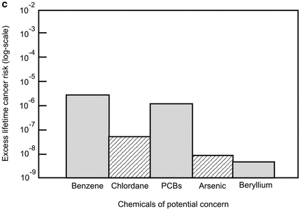
  (a) Vertical bar chart illustration of risk summary results. (b) Vertical bar chart illustration of risk summary results: illustrative presentation of the relative contribution of individual chemicals to overall hazard index estimates associated with a hypothetical public water supply system. (c) Vertical bar chart illustration of risk summary results: illustrative presentation of the relative contribution of individual chemicals to overall cancer risk estimates associated with a hypothetical public water supply system (semi-log plot)

• Variety of relational plots , such as shown in Figs. 11.4, 11.5, and 11.6 to illustrate various graphical relationships used to characterize risk associated with chemical exposure problems.

  Fig. 11.4

  

  Illustrative sketch of the effects of choice of exposure scenarios on dose and risk estimates

  Fig. 11.5

  

  Illustrative sketch of the variation of estimated cancer risks with distance from contaminant source: a semi-log plot of cancer risk estimates from receptor exposures to benzene in groundwater at several different locations downgradient of a release source

  Fig. 11.6

  

  Illustrative sketch of the variation of estimated hazard index with distance from contaminant source: an arithmetic-scale plot of hazard index estimates from receptor exposures to ethylbenzene in groundwater at several different locations downgradient of a release source

This listing is by no means complete; other novel representations that may consist of variations or convolutions of the above may indeed be found to be more appropriate and/or useful for some case-specific applications.

5 Risk Characterization in Practice and the Cumulative Risk Assessment Paradigm

A primary aim of risk assessment should be to inform decision-makers about the public health implications of various strategies for reducing receptor/populations exposures to the totality of environmental stressors. And yet, oftentimes, risk assessment applications seem centered on simply evaluating risks associated with individual chemicals in the context of regulatory requirements or isolated actions. In fact, it has become apparent that such a narrow focus does not accurately capture the risks associated with true exposure, given that simultaneous exposure to multiple chemical and nonchemical stressors seems inevitable in contemporary societies—and of course further to other factors that could influence receptor or population vulnerability as well (NRC 2009). This, therefore, calls for the concept of ‘cumulative risk assessment’—that may essentially be deemed as helping add a more holistic dimension to the risk characterization process.

Cumulative risk may be formally defined as the combination of risks posed by the aggregate exposure to multiple agents or stressors—whence aggregate exposure is exposure by all routes and pathways, and from all sources of each given agent or stressor (USEPA 2003a; NRC 2009). In this context, chemical, biologic, radiologic, physical, and psychological/psychosocial stressors are all recognized as affecting human health—and thus are potentially addressed in the multiple-stressor, multiple-effects assessments (Callahan and Sexton 2007; NRC 2009). Cumulative risk assessment may therefore be defined as the analysis, characterization, and possible quantification of the combined risks to health and/or the environment posed by multiple agents or stressors (USEPA 2003a; NRC 2009). That said, it is also noteworthy that cumulative risk assessment can involve qualitative analyses, and is not necessarily always wholly quantitative—recognizing that even limited or simple qualitative analyses may be sufficient at times to discriminate among competing risk management options (Callahan and Sexton 2007; USEPA 2003a; NRC 2009). Consequently, the cumulative risk assessment process would typically consist of the evaluation of an array of stressors (chemical and nonchemical) in order to characterize (quantitatively to the extent possible) human health or ecologic effects, taking account of such factors as vulnerability and background exposures (NRC 2009). [By the way, where this becomes the broader focus for particular program, ‘cumulative impact assessment’ would consider a wider array of end points, including effects on historical resources, quality of life, community structure, and cultural practices, some of which may not lend themselves to the ‘traditional’ quantification process/paradigm per se (CEQ 1989; NRC 1983).]

In spite of the fact that cumulative risk assessment by definition might consider psychosocial, physical, and other factors, most contemporary cumulative risk assessments do not tend to formally incorporate nonchemical stressors. Indeed, it is apparent that cumulative risk assessments have generally not quite attained the potential implied by the true definition—mainly because there has been less than optimal formal consideration of nonchemical stressors, aspects of vulnerability, background processes, and other factors that could be of interest to stakeholders concerned about effects of cumulative exposures (NRC 2009). All these may, in large part, be due to the fact that data tends to be inadequate to address most nonchemical stressors issues; but then, such omission also means that cumulative risk assessment will usually end up having a much narrower scope than could be expected or desired by many stakeholders (NRC 2009). Anyhow, despite all the apparent difficulties and/or complications to be anticipated in a typical problem situation, approaches to incorporate nonchemical stressors into cumulative risk assessment are not infeasible.

Meanwhile, cumulative risk assessments to date have mostly focused on aggregate chemical exposure assessment—and have generally not considered nonchemical stressors. Still, it should be explicitly recognized here that, analyses of chemical mixtures constitute only one component of cumulative risk assessment (even when the prospects for synergistic or antagonistic interactions that may affect the shape of the dose-response relationship of the individual chemicals are taken into consideration); indeed, for a truly comprehensive/holistic cumulative risk appraisal, other multiple stressors may have to be properly accounted for. That said, it is notable that the approach to evaluate cumulative risk posed by multiple chemicals with similar MOAs has been developed reasonably well (although with generally modest treatment of synergistic and antagonistic effects).

Cumulative risk assessment has also been used to determine the risks posed by baseline exposures, rather than the benefits of various risk management strategies—and this use has implications for the methods developed and their interpretations; for instance, NRC (2009) notes that some of the omissions can be attributed to the fact that formal consideration of numerous simultaneous chemical, physical, and psychosocial exposures with evaluation of background disease processes and other dimensions of vulnerability could quickly become analytically intractable if the standard risk assessment paradigm is followed—both because of the computational burden, and because of the likelihood that important exposure and dose-response data will be missing. Indeed, cumulative risk assessment requires extensive information beyond chemical toxicity and MOAs, including aggregate exposure data and information on population characteristics and nonchemical stressors—albeit, in the long run, despite the fact that there may be numerous theoretical combinations of exposures, only a subset will be relevant in choosing among various intervention options for a well-defined problem (NRC 2009).

Finally, it is worth mentioning here that, although it is generally preferable to have quantitative information as the primary health risk characterization/assessment outputs, it will often be useful enough to provide qualitative information about potential health effects when risks cannot be fully quantified. Furthermore, it should prove quite useful to incorporate appropriate terminologies that distinguish the full discussion of possible health effects from the myriad other effects that may be considered in a cumulative impact assessment (NRC 2009); indeed, any such undertakings should be such that, at the end of the day, it would be seen as serving a reasonably important role with regards to the decision on hand.

Bibliography

Bogen, K. T. (1994). A note on compounded conservatism. Risk Analysis, 14, 379–381.
Callahan, M. A., & Sexton, K. (2007). If cumulative risk assessment is the answer, what is the question? Environmental Health Perspectives, 115(5), 799–806.
CAPCOA. (1990). Air toxics “Hot Spots” program. Risk assessment guidelines. California: California Air Pollution Control Officers Association (CAPCOA).
CDHS. (1986). The California site mitigation decision tree manual. Sacremento, CA: California Department of Health Services (CDHS), Toxic Substances Control Division.
Clayton, C. A., Pellizari, E. D., & Quackenboss, J. J. (2002). National human exposure assessment survey: Analysis of exposure pathways and routes for arsenic and lead in EPA Region 5. Journal of Exposure Analysis and Environmental Epidemiology, 12(1), 29–43.
Cohrssen, J. J., & Covello, V. T. (1989). Risk analysis: A guide to principles and methods for analyzing health and environmental risks. Springfield, VA: National Technical Information Service (NTIS), US Dept. of Commerce.
DTSC. (1994a). CalTOX, A multimedia exposure model for hazardous waste sites. Sacramento, CA: Office of Scientific Affairs, CalEPA/DTSC.
DTSC. (1994b). Preliminary endangerment assessment guidance manual (A guidance manual for evaluating hazardous substance release sites). Sacramento, CA: California Environmental Protection Agency, Department of Toxic Substances Control (DTSC).
IARC. (1987). IARC monographs on the evaluation of carcinogenic risks of chemicals to humans: Overall evaluations of carcinogenicity, Supplement 7. Lyon, France: International Agency for Research on Cancer (IARC).
Johnson, B. L., & Jones, D. E. (1992). ATSDR's activities and views on exposure assessment. Journal of Exposure Analysis and Environmental Epidemiology, Suppl., 1, 1–17.
Klaassen, C. D. (Ed.). (2001). Casarett and Doull’s toxicology: The basic science of poisons (6th ed.). New York: McGraw-Hill.
Kodell, R. L., & Chen, J. J. (1994). Reducing conservatism in risk estimation for mixtures of carcinogens. Risk Analysis, 14, 327–332.
NRC. (1983). Risk Assessment in the Federal Government: Managing the Process, National Research Council, Committee on the Institutional Means for Assessment of Risks to Public Health. Washington, DC: National Academy Press.
NRC. (1991a). Environmental Epidemiology (Public Health and Hazardous Wastes). Washington, DC: National Academy Press.
NRC. (1991b). Frontiers in Assessing Human Exposure to Environmental Toxicants. Washington, DC: National Academy Press.
NRC. (1991c). Human Exposure Assessment for Airborne Pollutants: Advances and Opportunities. Washington, DC: National Academy Press.
NRC. (2009). Science and decisions: Advancing risk assessment. Washington, DC: Committee on Improving Risk Analysis Approaches Used by the U.S. EPA The National Academies Press.
NTP. (1991). Sixth annual report on carcinogens, National Toxicology Program (NTP). Washington, DC: US Department of Health and Human Services, Public Health Service.
Safe, S. H. (1998). Hazard and risk assessment of chemical mixtures using the toxic equivalency factor approach. Environmental Health Perspectives, 106(Suppl.4), 1051–1058.
Shields, P. G., & Harris, C. C. (1991). Molecular epidemiology and the genetics of environmental cancer. Journal of American Medical Association, 266, 681–687.
Slob, W. (1994). Uncertainty analysis in multiplicative models. Risk Analysis, 14, 571–576.
USEPA (US Environmental Protection Agency). (1984a). Approaches to risk assessment for multiple chemical exposures (EPA-600/9-84-008), Environmental Criteria and Assessment Office, US Environmental Protection Agency (USEPA), Cincinnati, OH.
USEPA. (1986a). Ecological risk assessment. Hazard Evaluation Division Standard Evaluation Procedure, Washington, DC.
USEPA. (1986b). Guidelines for the health risk assessment of chemical mixtures (EPA/630/R-98/002), Risk Assessment Forum, Office of Research and Development, US Environmental Protection Agency (USEPA), Washington, DC.
USEPA. (1986c). Guidelines for carcinogen risk assessment (EPA/630/R-00/004), September 1986. US EPA, Office of Research and Development, National Center for Environmental Assessment, Washington, DC.
USEPA. (1986d). Guidelines for mutagenicity risk assessment (EPA/630/R-98/003), Risk Assessment Forum, Office of Research and Development, USEPA, Washington, DC.
USEPA. (1986e). Methods for assessing exposure to chemical substances, volume 8: Methods for assessing environmental pathways of food contamination (EPA/560/5-85-008), Exposure Evaluation Division, Office of Toxic Substances, Washington, DC.
USEPA. (1986f). Superfund public health evaluation manual (EPA/540/1-86/060), Office of Emergency and Remedial Response, Washington, DC.
USEPA. (1989a). Exposure factors handbook (EPA/600/8-89/043), Office of Health and Environmental Assessment, Washington, DC.
USEPA. (1989d). Methods for evaluating the attainment of cleanup standards. Volume I: Soils and solid media. EPA/230/2-89/042. Office of Policy, Planning and Evaluation, Washington, DC.
USEPA. (1992a). Dermal exposure assessment: Principles and applications. EPA/600/8-91/011B, Office of Health and Environmental Assessment, US EPA, Washington, DC.
USEPA. (1992b). Framework for ecological risk assessment. EPA/630/R-92/001, February, 1992, Risk Assessment Forum, Washington, DC.
USEPA. (1992c). Guidance for data useability in risk assessment (Parts A & B), Publication No. 9285.7-09A&B, Office of Emergency and Remedial Response, USEPA, Washington, DC.
USEPA. (1992d). Guidelines for exposure assessment, EPA/600/Z-92/001, Risk Assessment Forum, Office of Research and Development, Office of Health and Environmental Assessment, USEPA, Washington, DC.
USEPA. (1992e). Supplemental guidance to RAGS: Calculating the concentration term. Publication No. 9285.7-08I, Office of Emergency and Remedial Response, USEPA, Washington, DC
USEPA. (1994a). Ecological risk assessment issue papers. EPA/630/R-94/009, Risk Assessment Forum, Washington, DC.
USEPA. (1994b). Estimating exposures to dioxin-like compounds. EPA/600/6-88/005Cb, Office of Research and Development, USEPA, Washington, DC.
USEPA. (1994c). Estimating radiogenic cancer risks. EPA 402-R-93-076, USEPA, Washington, DC.
USEPA. (1994d). Guidance for the data quality objectives process. EPA/600/R-96/055. Office of Research and Development, Washington, DC.
USEPA. (1994e). Guidance manual for the integrated exposure uptake biokinetic model for lead in children. EPA/540/R-93/081, Office of Emergency and Remedial Response, US Environmental Protection Agency (USEPA), Washington, DC.
USEPA. (1994f). Radiation site cleanup regulations: Technical support document for the development of radionuclide cleanup levels for soil. EPA 402-R-96-011A, September 1994.
USEPA. (1994g). Methods of derivation of inhalation reference concentrations and application of inhalation dosimetry. Office of Research and Development, Research Triangle Park, NC.
USEPA. (1996a). Guidelines for reproductive toxicity risk assessment. EPA/630-96/009, USEPA, Washington, DC.
USEPA. (1996b). Interim approach to assessing risks associated with adult exposures to lead in soil. US Environmental Protection Agency (USEPA), Washington, DC.
USEPA. (1996c). PCBs: Cancer dose-response assessment and application to environmental mixtures. EPA/600/P-96/001F, September 1996, National Center for Environmental Assessment, Office of Research and Development, U.S. Environmental Protection Agency, Washington, DC.
USEPA. (1996d). Radiation exposure and risk assessment manual. EPA 402-R-96-016, US Environmental Protection Agency (USEPA), Washington, DC.
USEPA. (1996e). Soil screening guidance: Technical background document, EPA/540/R-95/128. Office of Emergency and Remedial Response, Washington, DC.
USEPA. (1996f). Soil screening guidance: User’s Guide, EPA/540/R-96/018. Office of Emergency and Remedial Response, Washington, DC.
USEPA. (1997a). Ecological risk assessment guidance for superfund: Process for designing and conducting ecological risk assessments (ERAGS, EPA 540-R-97-006, OSWER Directive # 9285.7-25, June 1997), US Environmental Protection Agency, Washington, DC.
USEPA. (1997b). Establishment of cleanup levels for CERCLA sites with radioactive contamination. OSWER Directive 9200.4-18, August 1997.
USEPA. (1997c). Estimating radiogenic cancer risks. USEPA, Washington, DC.
USEPA. (1997d). Exposure factors handbook, Volumes I through III. EPA/600/0-95-002Fa, Fb, Fc, Office of Research and Development, USEPA, Washington, DC.
USEPA. (1997e). Guiding principles for Monte Carlo analysis. EPA/630/R-97/001, Office of Research and Development, Risk Assessment Forum, USEPA, Washington, DC.
USEPA. (1997f). Policy for use of probabilistic analysis in risk assessment. EPA/630/R-97/001, Office of Research and Development, USEPA, Washington, DC.
USEPA. (1997g). The lognormal distribution in environmental applications. EPA/600/r-97/006, Office of Research and Development/Office of Solid Waste and Emergency Response, USEPA, Washington, DC.
USEPA. (1997h). Users guide for the Johnson and Ettinger (1991) model for subsurface vapor intrusion into buildings. Office of Emergency and Remedial Response, USEPA, Washington, DC.
USEPA. (2000). Science policy handbook: Risk characterization. Science Policy Council, Washington, DC; EPA/100/B/00/002.
USEPA. (2003a). Framework for cumulative risk assessment. EPA/600/P- 02/001F. National Center for Environmental Assessment, Risk Assessment Forum, U.S. Environmental Protection Agency, Washington, DC.
USEPA. (2004a). Community air screening how-to manual. A step-by-step guide to using risk-based screening to identify priorities for improving outdoor air quality. EPA 744-B-04-001. U.S. Environmental Protection Agency, Washington, DC.
USEPA. (2004b). Risk assessment guidance for Superfund: Volume 1—Human health evaluation manual (Part E, supplemental guidance for dermal risk assessment). Final, July 2004. EPA/540/R/99/005. Office of Emergency and Remedial Response, US Environmental Protection Agency, Washington, DC.
USEPA. (2004c). Example Exposure Scenarios. EPA/600/R-03/036. Center for Environmental Assessment, US Environmental Protection Agency, Washington, DC.
USEPA. (2004d). Risk assessment principles and practices. Staff Paper, EPA/100/B-04/001. Office of the Science Advisor, U.S. Environmental Protection Agency, Washington, DC.
USEPA. (2004e). User’s guide for evaluating subsurface vapor intrusion into buildings. Office of Emergency and Remedial Response, Washington, DC.
USEPA. (2004f). Air quality criteria for particulate matter: Volume II. Office of Research and Development, Washington, D.C. EPA/600/P-95/001bF.
USEPA. (2004g). An examination of EPA risk assessment principles and practices. Washington, DC: Office of the Science Advisor, Environmental Protection Agency.
USEPA. (2005a). Guidelines for Carcinogen risk assessment. EPA/630/P-03/001B, March 2005. US EPA, Office of Research and Development, National Center for Environmental Assessment, Washington, DC.
USEPA. (2006a). Approaches to the application of physiologically based pharmacokinetic (PBPK) models and supporting data in risk assessment (Final Report), EPA/600/R-05/043F. National Center for Environmental Assessment, NCEA, US Environmental Protection Agency, Washington, DC.
USEPA. (2009). Risk assessment guidance for superfund Volume I: Human health evaluation manual (Part F, Supplemental Guidance for Inhalation Risk Assessment), EPA-540-R-070-002, OSWER 9285.7-82, January 2009, Office of Superfund Remediation and Technology Innovation, Environmental Protection Agency Washington, DC.
USEPA. (2000b). Supplementary guidance for conducting health risk assessment of chemical mixtures. U.S. Environmental Protection Agency, Washington, DC. EPA/630/R-00/002. August
CEQ. (1989). Risk analysis: A guide to principles and methods for analyzing health and environmental risks, Council on Environmental Quality. Washington, D.C. NTIS: PB89-137772.
Author information
Authors and Affiliations
Rights and permissions
Copyright information
© 2017 Springer Science+Business Media B.V.
About this chapter
Cite this chapter
Asante-Duah, K. (2017). Chemical Risk Characterization. In: Public Health Risk Assessment for Human Exposure to Chemicals. Environmental Pollution, vol 27. Springer, Dordrecht. https://doi.org/10.1007/978-94-024-1039-6_11
Download citation
DOI: https://doi.org/10.1007/978-94-024-1039-6_11
Published:
Publisher Name: Springer, Dordrecht
Print ISBN: 978-94-024-1037-2
Online ISBN: 978-94-024-1039-6
eBook Packages: Earth and Environmental ScienceEarth and Environmental Science (R0)