
Abstract
This contribution presents an evaluation of still unexplored potentials, limitations and technical details of µ-XRF element scanning particularly for varved sediment analyses using the vacuum device EAGLE III XL. For this case study a 33 cm long interval of exceptionally well-preserved sub-millimetre scale calcite varves of the interglacial lake deposits from Piànico has been selected. In addition to the demonstration of the very good repeatability of XRF element scans, one focus of this paper is on discussing a suitable scanner resolution in terms of a compromise between short analyses times and a resolution that allows capturing the geochemical signature even of seasonal sub-layers. By combining scanner data with microscopic sediment inspection geochemical signatures of various micro-facies as, for example, varves, detrital layers and matrix-supported and clay layers are explored. The potential of counting varves using the seasonal signature of specific elements is discussed and potential error sources are disclosed by comparison with microscopic varve counts. Detailed grid- µXRF-scanning provides for the first time an insight into the internal structure of varves presented as high-resolution 3D-images. Finally, an approach of calibrating scanner data through comparison with ICP-MS analyses is introduced. Sensitivity factors for each element have been defined as ratios between mean count rates and bulk element concentrations.
Access provided by Autonomous University of Puebla. Download chapter PDF
Keywords
Introduction
The increasing demand over recent decades for spatially resolved information from sediment cores has led to the development of several XRF scanning instruments for non-destructive and continuous analysis (Jansen et al. 1998; Koshikawa et al. 2003; Croudace et al. 2006; Haschke 2006; Richter et al. 2006), resulting in an increased number of publications presenting results of sediment core analyses from one per year in the 1990s to 41 in 2009 (Croudace and Rothwell 2010).
µ-XRF scanning allows the determination of the downcore element composition of sediments by continuous single line scanning along split cores of sediments and sediment blocks embedded in epoxy resin (e.g. Röhl and Abrams 2000; 2001; Brauer et al. 2008a). Latest generation core scanners provide spatial resolutions down to 100 µm but, depending on the focussing device of the µ-XRF instrument, the spot size can be narrowed down to as little as 50 µm (Haug et al. 2003; Haschke 2006; Brauer et al. 2007a, 2008a; Gennari et al. 2009). Typical spot sizes applied for sediment core analyses vary between 0.5 mm (Yancheva et al. 2007) and a few cm (Richter et al. 2001). For resin-embedded sediment blocks and dry samples spot sizes down to 20 µm have been reported (Shanahan et al. 2008).
Key parameters influencing the signal intensity are shown in Table 12.1. Apart from the scanner setup, such as X-ray tube type (e.g. Cr, Mo, Rh), tube voltage and current, spot and step size and dwell time, numerous physical and chemical parameters significantly influence the generation and detection of the fluorescence radiation of the individual elements (Weltje and Tjallingii 2008; Francus et al. 2009). Key considerations include experimental characteristics like (i) use of a protective cover foil (Ge et al. 2005; Böning et al 2007; Tjallingii et al. 2007), (ii) X-ray beam focussing device based on a slit (Avaatech scanner), an X-ray capillary waveguide (Itrax) or by means of a polycapillary lens geometry (EAGLE III XL), (iii) measuring through air (SXAM, Katsuta et al. 2007), under vacuum (EAGLE III XL), through a hollow prism flushed with He (Avaatech scanner) or directly flushing the area between sample surface and detector window with He (EAGLE III BKA, Yancheva et al. 2007), (iv) software, data acquisition and peak processing techniques, background subtraction, sum-peak and escape-peak correction, deconvolution and peak integration and (v) sample characteristics like matrix composition, dilution effect by organic matter (Löwemark et al 2011), interstitial water content (Böning et al. 2007), porosity, grain-size, surface roughness, irregular geometric shape of layers and heterogeneity within individual layers. The importance of these parameters increases rapidly with decreasing spot sizes. Thus the conversion of core scanner output data (element intensities or count rates) into absolute element concentrations still remains a major problem of µ-XRF core scanning.
Several attempts have been made to convert element intensities or count rates into element concentrations by comparison with concentration data obtained by conventional chemical analyses of bulk samples, taken from the core at the same positions of the µ-XRF linescans (Jansen et al. 1998; Kido et al. 2006; Böning et al. 2007). However, resulting regression lines often reveal poor correlation and seldom pass the origin (Weltje and Tjallingii 2008). The log-ratio model of Weltje and Tjallingii (2008) seems to provide a more accurate and precise calibration method, although one has to keep in mind that calibration factors derived from one type of sediment are not readily applicable to other sediments (Weltje and Tjallingii 2008). This observation mandates that for reliable calibration purposes a reasonable large number of bulk samples of each core must be taken for conventional chemical analyses (e.g. ICP-AES, ICP-MS, AAS, XRF), which is not feasible for routine work. For high-resolution measurements (spot size < 100 µm) of finely laminated sediments (lamina width << 1 mm) the preparation of discrete bulk samples for chemical analyses is extremely difficult or nearly impossible.
In spite of the obvious advantages of the µ-XRF method (i.e. resolution, continuity of the record, non-destructive character, marginal sample preparation) , interpretation of µ-XRF data is not straightforward. This study aims to evaluate the capabilities and limitations of the µ-XRF technique at high-resolution. For this purpose, we have chosen as test material a varved lake sediment sequence from the Piànico palaeolake (Italy) which displays exceptionally well-preserved annual laminations (Brauer et al. 2008b), a relatively simple varve structure and well-defined event layers (Mangili et al. 2005). The detailed information obtained from microfacies analyses minimises complications resulting from more complex sedimentological settings and makes this sequence ideal for this feasibility study. Bulk sample analyses by inductively-coupled plasma mass spectrometry (ICP-MS) for selected sediment intervals, which have been analysed by µ-XRF scanning, is applied to estimate the relation between µ-XRF count rates and element concentrations .
Study Site and Sediments
The sediments of the Piànico palaeolake (45° 48′ N, 10° 2′ E, Fig. 12.1a) are visible along outcrops in the Borlezza River valley (Southern Alps, Italy). The bedrock around the palaeolake consists mainly of Upper Triassic dolomitic rocks (Dolomia Principale) and limestones belonging to the Calcare di Zorzino Unit (Provincia di Bergamo 2000).

a Simplified geological map of the area of the Piànico palaeolake (modified after Casati 1968). The dashed blue line marks the reconstructed extension of the palaeolake. b Simplified stratigraphic column of the varved lacustrine interglacial unit (BVC; stands for the local stratigraphic term ‘Banco Varvato Carbonaticoa’ i.e. Carbonate Varved Bed) and of the upper unit (MLP; stands for the local stratigraphic term ’Membro di La Palazzina’ i.e. La Palazzina Member) that is characterised by rapid alternation of detrital to endogenic calcite dominated intervals. c Optical image of the studied sample taken from the “main section” outcrop. d SEM image of a summer layer, showing the endogenic calcite crystals that form up to 98 % of a single varve
Within the palaeobasin the lacustrine Piànico Formation has been preserved (Moscariello et al. 2000). For this study only the unit named BVC (“Banco Varvato Carbonatoa” i.e. Carbonatic Varved Bed) is considered. This unit mainly consists of biogeochemically precipitated calcite varves (Fig. 12.1b) that formed under interglacial conditions. The age of these deposits has been determined by tephrochronology at ca 400 ka BP thus coinciding with Marine Isotope Stage (MIS) 11 (Brauer et al. 2007b). Although this age has been questioned (Pinti et al. 2007) it still appears to be the most realistic estimate (Brauer et al 2007c). Field varve counting of the entire unit yielded a minimum duration of ca. 15500 varve years for this period of peak interglacial conditions (Mangili et al. 2007).
The varves (Fig. 12.1c) are composed of two laminae: a light spring-summer lamina of biogeochemically precipitated calcite (Fig. 12.1d), and a dark autumn-winter lamina dominated by organic matter, diatom debris and scattered detrital grains (Brauer et al. 2008b). The mean varve thickness varies between 0.2 and 0.8 mm. Four detrital layer facies, intercalated in the varve succession, have been described: 0.03 mm–6 cm thick detrital layers composed of Triassic dolomite, matrix supported layers (Mangili et al. 2005) consisting of medium to coarse silt-sized detrital grains embedded in a matrix of fine-grained isomorphic calcite, clay layers and a tephra layer rich in volcanic glass (Brauer et al. 2007b). Detrital layers are interpreted as triggered by extreme rainfall events (Mangili et al. 2005).
Materials and Methods
Sample Collection and Preparation
Sediment blocks were collected from the Main Section (Fig. 12.1), using 33 × 5 × 5 cm (L × W × H) special stainless steel boxes with removable side walls. In the laboratory the sample blocks were slowly dried at room temperature to avoid quick shrinkage and cracking, and then covered with Araldite® 2020 transparent epoxy resin. In this way, the resin impregnated the outer 1–2 mm of the sediments. Cutting the sample blocks along their length axis yielded corresponding plains for both thin section analyses and µ-XRF scanning. This is a crucial prerequisite for precise comparison of microscope and element scanning data. The surface of the sediment slice used for µ-XRF analyses was again slowly dried and dry-polished in order to obtain a smooth surface without further resin impregnation.
Micro X-ray Fluorescence (µ-XRF) Spectrometry
For this study the high-resolution µ-XRF spectrometer EAGLE III XL (Röntgenanalytik Messtechnik GmbH, Germany) was used. The system specifications are summarized in Table 12.2. Major features of the instrument are described in more detail by Haschke et al. (2002) and Haschke (2006).
Spectral data were processed (including background correction, escape-peak correction, peak deconvolution and peak area integration) using standard EDAX software (Vision). The resulting data represent element intensities expressed as count rates (counts per second, cps) for individual spots along the scanned line.
The EAGLE III XL spectrometer differs significantly from the worldwide leading X-ray -core scanners Itrax and Avaatech in four major respects.
-
a.
The large vacuum chamber allows the measurement of dry samples under vacuum that improves the detection efficiency of low Z elements like Mg , Al and Si. For the Itrax core scanner Al is the lightest element which can be measured applying reasonable exposure times (Löwemark et al. 2011). This applies to the Avaatech core scanner, too (Tjallingii et al. 2007). For the Itrax core scanner the Cr tube is recommended for detection of lighter elements.
-
b.
The polycapillary lens captures a large angle of the primary radiation beam and focuses it onto a small area on the sample surface, producing a nearly circular X-ray spot. The VariSpot-system of the EAGLE III XL spectrometer enables the variation of the spot size by moving tube and capillary-optic in direction of the axis of the optics without significant changes of the count rate (for a homogeneous sample) because the total number of the primary X-ray photons remains constant (Haschke et al. 2002) while the photon density (number of X-ray photons per cm2) changes. A further increase of the “spot-size” may be achieved by raster-methods controlled by the software. The circular spot with down to 50 µm diameter or less is particularly suitable for mapping experiments. An additional advantage of the small circular spot becomes apparent for samples with inclined layer structure. Depending on the angle between the layers and the sedimentation direction the resulting resolution might be decreased when applying instruments using rectangular X-ray beams with lengths of ca. 1 cm or more. This is significantly less pronounced for the small circular spot.
-
c.
A real-time video camera shows the sample image for each measured sample point for which an optical image can be stored for later examination. This enables the precise relocation of the X-ray beam on the sample, even after reloading a sample. The stored images allow inspection of sampling points of “outlier” values in element profiles in order to identify sample disturbances such as cracks or holes.
-
d.
The computer controlled X-Y-Z-sample stage enables the operator to run predefined scanning lines in all three dimensions to avoid scanning across sample intervals which exhibit obvious disturbances. The autofocus function adjusts the z-position of the sample stage to maintain a constant distance between sample surface and detector.
µ-XRF measurements for this feasibility study were performed under vacuum on the fresh sediment surface of one 33 cm sediment block (sample PNC 17 of Piànico palaeolake , Italy). Figure 12.2 shows an optical scanning image of the sample with indications for two independent scanned lines (black lines), five mapped areas (black boxes), and references to the figures where data for these measurements are presented. For single line measurements instrument settings were 40 kV tube voltage, 200 µA tube current, ca. 54 µm spot size, 50 µm step size and an integration time of 60 s (livetime). Taking into account an average dead time of 35 % and time for sample movement and data storage, this results in a total measurement time of approximately 90 s for each sampling point.

Optical image of the 33 cm long sediment block of sample PNC 17 taken from “main section” outcrop with indications for the different scanned lines (black lines), mapping areas (black boxes), and references to the figures where data are presented. cl clay layer, dl detrital layer, msl matrix supported layer
Data for element mapping were collected at five characteristic intervals of the PNC 17 sediment block (Fig. 12.2). At each selected interval 61 parallel lines were scanned for either 3 mm (four sites) or 6 mm (one site) lengths. The distance between individual sampling points was 50 µm in x- and y-directions. These analyses were carried out using a tube voltage of 40 kV, a tube current of 250 µA, a spot size of ca. 54 µm and a step size of 50 µm, resulting in 3721 data points for a 3 × 3 mm matrix and 7381 data points for the 3 × 6 mm matrix. For an exposure time of 30 s (lifetime) the total analysis times were 46 h and 93 h for 3 × 3 mm and 3 × 6 mm scanned areas, respectively.
For calibration purposes two reference samples, limestone KH (Zentrales Geologisches Institut of the former GDR) and a 1:1 mixture (by mass) of KH and the basalt BM (CRPG-BRGM, France), were measured. The reference samples were prepared as pressed powder pellets from homogeneous sample powder (grain-size < 65 µm). A 1 × 1 cm raster was measured with a distance of 1 mm between each spot, resulting in 100 measuring points. To minimize a grain-size influence a 250 µm spot was used. Tube settings are the same as for linescans of the Piànico samples.
Inductively Coupled-Plasma Mass Spectrometry (ICP-MS)
Eighteen “bulk” subsamples were analysed by inductively coupled plasma-mass spectrometry (ICP-MS) subsequently being scanned at 50 µm resolution using the EAGLE III XL. The ICP-MS procedure is described in detail by Dulski (2001). ICP-MS samples were obtained by scratching the fresh surface of sediment blocks with a razor blade. Each ICP-MS sample contains five varves. ICP-MS bulk concentration data has been used for comparison with the mean of the µ-XRF count rates (cps) of the corresponding scanning intervals of five varves whereby Mg, Al, Ca, Ti, Fe and Sr were determined using both techniques.
Results
Repeatability of the µ-XRF Measurements
To demonstrate the repeatability of the µ-XRF measurements with the EAGLE III system applying 50 µm spot size on a separate Piànico sample a single 30 cm scanning line was measured twice. For better viewing Fig. 12.3 shows results for a 0.5 cm section only. The consistency of replicate profiles of the same scanning line for Ca, Si and Mg demonstrates the good repeatability of the µ-XRF measurements. Even Mg , showing low count rates (< 10 cps) due to low sensitivity and concentration, can be clearly distinguished from instrumental noise.

Ca, Si and Mg intensity profiles for a duplicate measurement of a single scanning line (50 µm spot- and step size) on Piànico sediment sample PNC W053. The consistence of both profiles for each element demonstrates the good repeatability of the µ-XRF measurements. Even Mg, showing low count rates (< 10 cps) due to low sensitivity, can be clearly distinguished from instrumental noise
Scanner Resolution
Selecting the appropriate scanner resolution mainly depends on the sedimentological characteristics of the sediment. Higher resolution (smaller spot and shorter step sizes) results in more data points for individual layers and better statistical characterization of these layers. However, this clearly leads to a significant increase of measurement time for each sample. Applying 50 µm resolution and a dwell time of 60 s (life time), which are typical for analyses with our EAGLE III system, the duration for the measurement of 10 cm is about 50 h. Such duration is not practicable for routine measurements of long sediment sequences.
To optimize the discrimination between the various layers and to minimize measurement times we have determined the influence of the scanning resolution on the µ-XRF element profiles by scanning two 5-cm intervals using 50, 100, 200 and 500 µm spots and corresponding step sizes. One line (line A, Fig. 12.2) crosses an interval of thick varves while the other (line B, Fig. 12.2) intersects an interval of thinner varves. Results of the 5-cm long sequences for Ca (representing spring-summer layers, dominated by calcite) and Si (representing autumn-winter layers, dominated by diatom debris and detrital grains) are shown in Fig. 12.4 together with the corresponding thin section images. With increasing spot size the annual signatures in both profiles become progressively less distinct as indicated by a decreasing discrimination of individual peaks and a progressive lowering of the oscillation amplitude between minima and maxima of neighboured peaks. As expected, such signal degradations are less pronounced for the sample sequence with thicker varves (Fig. 12.4c, e, g) than for the sequence with thinner varves (Fig. 12.4d, f, h). According to the sedimentary features the 50 µm spot (centred on a thin dark autumn-winter layer, Fig. 12.4a and b) covers an area predominantly consisting of the Si-rich autumn-winter layer while for the 500 µm spot more than 90 % of the spot area is represented by the Ca-rich spring-summer layer. This increase of the fraction of the thicker spring-summer layer within the spot area relative to the fraction of the autumn-winter layer leads to the reduction in the oscillation amplitudes for both elements (Fig. 12.4e–h). For both intervals (line A and B, Fig. 12.4) Ca profiles for 50 µm spots (blue lines in Fig. 12.4e and f) show a nearly flat upper base line of count rates between 3300 and 3700 cps and pronounced peaks dropping to lower count rates down to 600 cps. The opposite behaviour is observed for Si (red lines in Fig. 12.4g and h) with a relatively flat lower baseline between 60 and 100 cps and pronounced peaks rising up to 350 cps. Figure 12.5a, b, c, d, e, f, g, h shows a more detailed view of the profile structure for 0.5 cm intervals of both scanned sequences. The results clearly demonstrate that for both sequences spot sizes of 200 and 500 µm (Fig. 12.5c, d, g and h) are not suitable to resolve the Si-rich autumn winter layers from the Ca-rich spring-summer layers while using a 50 µ spot (Fig. 12.5a and e) distinct peaks for the thin autumn winter layers of both sequences are seen which are characterized by 5 to 10 points per peak (line A, Fig 12.5a) and 3 to 5 points per peak (line B, Fig. 12.5e). A 100 µm spot appears to be sufficient for the interval with thicker varves (Fig. 12.5b) but not for the sequence with thinner varves (Fig. 12.5f).

Thin section microscope image and various spot size areas (50, 100, 200, 500 µm diameter) compared to varve thickness (a and b), optical images of two five cm sequences of sample PNC 17 (c and d) with scanning line position (black lines) and Ca- (e and f) and Si- (g and h) intensity profiles using spot sizes of 50, 100, 200 and 500 µm (dark blue and dark red lines show 50 µm resolution). Ca profiles (e and f) are characterized by a relatively flat upper baseline and pronounced peaks dropping down to lower intensities while Si (g and h) shows the opposite behaviour with a relatively flat lower baseline and significant peaks to higher count rates. In profiles obtained with 500 µm spot- and step size (yellow line in e to h) the annual signature is partially masked because the spot area is dominated by nearly 90 % of the Ca-rich spring-summer layers (a and b)

Ca- (blue lines) and Si- (red lines) intensity profiles for two 0.5 cm sequences of scanning line A (a to d) and B (e to h) using spot sizes of 50 (a and e), 100 (b and f), 200 (c and g) and 500 µm (d and h), respectively. Background images are thin section scans taken with a standard flatbed scanner and polarized light. With increasing spot size the annual signal of Ca and Si in profiles of line A (thicker varves) and line B (thinner varves) partially or totally disappears, indicated by worse discrimination of individual peaks and a progressive decrease of the oscillation amplitude between minima and maxima of neighboured peaks
Sediment Microfacies in µ-XRF Data
The spatial element distributions within different types of microfacies are presented as 2D and 3D plots. We introduced 3D mapping to compare element intensities and microscope facies analyses of thin sections as a way to depict internal varve structure and as a tool to analyse lateral changes in µ-XRF scanning. For that purpose µ-XRF data have been gridded and plotted using the software Surfer, version 8.01.
Five major microfacies types were distinguished in the interglacial sediments of the Piànico palaeolake : (i) calcite varves, (ii) detrital layers, (iii) matrix supported layers, (iv) clay-rich layers, (v) and a tephra layer.
-
i.
Calcite varves: In the 2D (Fig. 12.6a) and 3D plots (Figs. 12.7 and 12.8) Ca, as proxy for endogenic calcite precipitation in spring and summer, shows the highest count rates with significantly lower values for the thin autumn-winter layers. Peaks in Si indicate the detrital and diatom debris of the autumn-winter layers. The other elements (Mg, Fe, Al, K, Sr and Ti) show generally very low count rates. Sr generally follows the Ca pattern, indicating the presence of Sr in calcite crystals, Mg accounts for detrital Triassic dolomite from the catchment (Mangili et al. (2010) and Al, K, Fe and Ti reflect the sporadic presence of clay particles settling out from suspended detrital material which most likely has been transported into the lake by a stream coming from the inner Alps in the North (Moscariello et al. 2000).
Fig. 12.6 
Thin section images of four different sediment sequences in PNC 17 and overlayed major element profiles. a Four varves (w = winter layer) and µ-XRF major element profiles (Mg*800, Ca, Si*20) for the same interval. Peaks in Ca coincide with the light summer layers, those of Si with the dark winter layers. b Thin section image of four varves and µ-XRF element profiles (Mg*800, Ca, Si*20). One varve includes a detrital layer (dl) which is indicated by the significant Mg peak just below the winter layer (peak for Si). c Thin section image of five varves and µ-XRF profiles (Mg*800, Ca, Si*20). One varve includes a matrix supported layer (ms) characterized by a constant and high Ca count rate across the whole layer. d Thin section image of the tephra layer included in the BVC unit and µ-XRF profiles (Ca, Si*20, K*10). The tephra layer is dominated by high and nearly constant Si and K signal intensities
Fig. 12.7 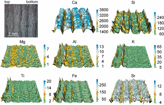
Thin section image and 3D µ-XRF element distribution maps (element intensities are expressed as counts per second) covering an area of 3 × 3 mm of thick varves. Ca and Sr peaks correspond to varve spring-summer layers composed mainly of endogenic calcite, Si peaks to autumn-winter layers dominated by diatom debris and scattered detrital grains. Al, K and Ti peaks are due to clay micro-fragments in the autumn-winter layers. Mg peaks reflect detrital dolomite grains of Triassic age washed into the lake from the catchment. These dolomite grains appear either scattered or enriched in winter and especially flood layers. (Mangili et al. 2005)
Fig. 12.8 
Thin section image and 3D µ-XRF element distribution maps (element intensities are expressed as counts per second) covering an area of 3 × 3 mm characterised by thin varves. Ca peaks correspond to varve spring-summer layers. Si peaks to autumn-winter layers. Al and K peaks are due to clay micro-fragments in the autumn-winter layers. Mg peaks reflect detrital dolomite grains of Triassic age washed into the lake from the catchment
-
ii.
Detrital layers: In the 2D plot (Fig. 12.6b) the presence of the detrital layer (dl) is marked by the broad peak of Mg , representing the Triassic dolomite originating from the catchment area as main component of detrital layers. The 3D maps of a sequence containing detrital layers (Fig. 12.9) show a four varve interval, where each summer layer includes one to two detrital layers. Further components of detrital layers are clay fragments characterized by the Al and K peaks.
Fig. 12.9 
Thin section image and 3D µ-XRF element distribution maps (element intensities are expressed as counts per second) covering an area of 3 × 3 mm of varves including four detrital layers. Ca peaks correspond to varve spring-summer layers, Si peaks to autumn-winter layers. Al and K peaks are due to clay micro-fragments present in the autumn-winter layers. Mg peaks are due to the presence of Triassic dolomite forming the detrital layers
-
iii.
Matrix supported layers: Matrix supported layers are indicated by elevated Ca values over the entire range of the layer. The 3D maps of a matrix supported layer (Fig. 12.10) clearly show an area of constant Ca values, interrupted only by a few isolated peaks in Si which result from isolated quartz grains. Mg, Al and K are generally low within the matrix supported layer.
Fig. 12.10 
Thin section picture and 3D µ-XRF element distribution maps (element intensities are expressed as counts per second) covering an area of 3 × 3 mm for a matrix supported layer characterized by high and constant Ca values. Above the Matrix Supported layer, the varved pattern starts again, with Ca peaks alternated with Si peaks. The peaks in Mg mark the presence of a detrital layer within the varve succession
-
iv.
Clay layers: Clay layers exhibit a very different element composition. The 3D plots (Fig. 12.11) show high count rates for Al and K, intermediate count rates for Si and Mg and low count rates for Ca. Such millimetre to centimetre thick clay layers only rarely occur in the Piànico record. Sub-mm thick layers of clay are sometimes present within a varve, mostly associated to autumn-winter layers (e.g. peaks in Al and K in Figs. 12.7, 12.8).
Fig. 12.11 
Thin section picture and 3D µ-XRF element distribution maps (element intensities are expressed as counts per second) covering an area of 6 × 3 mm of a sediment sequence containing two varves (Ca peaks on the right), a matrix supported layer (Mg rich, middle), and a thick clay layer (flat and high K and Al plateau on the left)
-
v.
Tephra layer (Fig. 12.6d ): The presence of a tephra layer within the varved sequence (Brauer et al. 2007b) is detected by an abrupt increase of Si and K count rates and a sudden drop of Ca count rates at the beginning of the tephra. The high Si and K count rates characterise the entire tephra layer, but the semiquantitative nature of µ-XRF scanner data limits any information about the volcanic source of the tephra. To discriminate between different volcanic sources and/or eruptions quantitative methods (e.g. microprobe analysis or laser ablation ICP-MS) must be applied.


A particular advantage of high-resolution µ-XRF is that even sub-millimetre-size features can be identified. A micro-dropstone within the varve succession (Fig. 12.12) is identified by high Mg count rates while the deformation of the autumn-winter layers below the micro-dropstone is evident in the Si distribution. Within the area of the micro-dropstone, Ca, which is also constituent of dolomite, shows intermediate intensity values (lower than in the varve spring-summer layers).

Optical image and 3D µ-XRF element distribution maps (element intensities are expressed as counts per second) for Ca, Mg and Si covering an area of a 3 × 5 mm sediment sequence containing a micro-dropstone inclusion. The varve succession has been deformed by the dolomite micro-dropstone. Ca peaks correspond to varve spring-summer layers, Si peaks to autumn-winter layers. Mg peak indicates the Triassic dolomite forming the dropstone
Intra-lamina Variability
µ-XRF measurements were generally carried out on single lines (50 µm wide) along the stratigraphic sequence. Due to internal lamina heterogeneity, variations in layer thickness along individual lamina and skewing of layers, resulting µ-XRF intensity profiles vary depending on the lateral position of the scanning line. 3D µ-XRF element mapping show that µ-XRF count rates in the direction perpendicular to the sedimentation direction scatter significantly (e.g. Figs. 12.7–12.12) and can vary by more than one order of magnitude. Figure 12.13 shows the Ca- and Si intensity profiles of 61 parallel scanning lines crossing a 3 mm sequence of thin varves. For each line a spot size of ca. 54 µm and step size of 50 µm was applied. The distance between each of the parallel lines was 50 µm. Intra-varve variability causes variations of the signal intensities for the peak minima (Ca, 500–2500 cps) and maxima (Si, 150–450 cps) of the autumn-winter layers. The shift of the peak position up to 300 µm and the variation in peak width (a few tens µm) result from both the non-vertical layer geometry and the variable thickness along the layers. Despite the observed variations between the individual profiles seven significant thin autumn-winter layers (Ca low, Si high) are identified in all linescans.

Ca- and Si intensity profiles of 61 parallel scanning lines crossing a 3 mm sequence of thin varves. Intra varve variability results in large variations of the signal intensity for the peak minima (Ca) and maxima (Si) of the autumn-winter layers. The observed shift of the peak position and the variation in peak width of the individual lamina are due to the skewed layer characteristic and the variable thickness along the layers, respectively. Despite the large variation of the individual profiles the seven significant thin autumn-winter layers (Ca low, Si high) within this sequence are identified by each scanning line
Varve Counting in µ-XRF Records
Due to the good correspondence between µ-XRF and microscope data an attempt was made to varve count based solely on µ-XRF Ca profiles (Fig. 12.14). Control counts on thin section with a petrographic microscope reveal a total of 39 varves between two well-defined marker layers. It was not possible to obtain the same number of varves by counting the Ca minima (more pronounced than the maxima) in the µXRF data (Fig. 12.14a). The causes for this discrepancy in this specific case were the presence of a matrix supported layer, one varve that wedging out laterally (Fig. 12.14b) and by varves with very thin winter layers.

a Thin section image and Ca profile of a 15 cm long varved sediment sequence. The dashed lines mark the correspondences between the thin section image and the µ-XRF curve (dark autumn-winter layer represented by Ca minima). The boxes highlight parts of the Ca curve where varve counting based on µ-XRF peaks is difficult because of a lack of clear variations in the Ca signal for the matrix supported layer (box 1) and an interval of 3 varve years which are not well distinguishable (box 2). b 3D µ-XRF Si map for a particular varve interval, showing an additional winter layer along the line x compared to line y
µ-XRF and ICP-MS Comparison
The results of ICP-MS analyses for 18 bulk-samples of the Piànico sediment block, each averaging 5 varves, are shown in Table 12.3. They reveal that Ca is the most abundant metallic element in all subsamples, with concentrations between 29 and 35 wt%. Mg, Al and Fe are present in the lower percentage range (between 0.1 and 1.3 wt%) and Ti and Sr present only in trace amounts (60–500 µg/g). Si could not be determined because it is lost during the chemical decomposition procedure to dissolve the solid samples and K could not be analysed by ICP-MS due to the interference from the large Ar peak resulting from the plasma gas.
Sensitivity factors (cps/wt%), defined as the ratio between the mean count rates and the corresponding bulk concentrations determined by ICP-MS, were calculated for each element. For Si and K sensitivity factors were calculated using the net count rates obtained by the µ-XRF measurements of the pressed powder pellets of the two reference samples (limestone KH and 1:1 mixture of KH and basalt BM) and their reference concentration values (Govindaraju 1994). The results presented (Table 12.4 and Fig. 12.15) demonstrate that the obtained sensitivity factors increase with atomic mass of the elements. The sensitivity factors for the various elements, established for the Piànico sediment, scatter considerably (relative standard deviation between 6 % for Ca and 34 % for Al) due to the low count rates and related low counting statistics for most of the elements. The calculated sensitivity factors obtained from the Piànico samples correlate reasonably well with those from the two reference samples KH and the 1:1 mixture of KH/BM.

Sensitivity factors (cps/wt%) for selected elements versus atomic mass number. Horizontal bars indicate the Piànico samples, the squares the standard KH and the circles the 1:1 mixture of KH/BM. For the EAGLE III system, equipped with a Rh X-ray tube, the sensitivity factors systematically increase with atomic mass from Mg to Sr
Discussion
The results of this study demonstrate that µ-XRF scanning is complementary to sediment micro-facies analyses because of the potential to provide geochemical data at seasonal resolution. In order to design optimal instrument setup it is crucial to make some fundamental considerations concerning measurement and data interpretation. Among those are repeatability, spatial resolution, time for measurement, sediment characteristics, homogeneity and continuity of lamina and calibration.
Duplicate measurements of the same scanning line on the Piànico sediment clearly prove that the observed uncertainties for our µ-XRF data are low and that they can be neglected for this study. Applying the 50 or 100 µm spot the observed relative variations of the count rates for each element between the different facies types of the Piànico sediments are significantly larger than the relative standard deviations of the measurement. This enables the discrimination of these facies types by the presented µ-XRF profiles.
The selected scanning resolution mainly depends on the sedimentation rate and the specific goals of the µ-XRF element scanning. Application of a larger spot size (lowering of the scanning resolution) results in a wider area over which the µ-XRF signal is integrated (Fig. 12.4a and b). Increasing spot sizes to values exceeding varve thickness prevents from resolving seasonal signals in annually laminated sediments. The reduction of µ-XRF count rate amplitudes (Figs. 12.4 and 12.5), measured at 500 µm resolution compared to 50 µm resolution results in smoothed curves that lack any high-frequency signals. The smoothing of the µ-XRF records at lower resolution also affects intensity ratios of elements. For 50 µm resolution the Ca/Si intensity ratio for the spring-summer layers is ca. 40 while the ratio for the autumn-winter layer is around 10. At 500 µm resolution Ca/Si intensity ratios range between 20 and 30 for both layer types.
Obviously, the selected scanning resolution also affects the time required for µ-XRF analyses. Therefore sedimentation rate determination by micro-facies analyses prior to µ-XRF analyses is a suitable tool to define the ideal and effective scanning resolution in terms of minimum analytical times and precisely adjusted data resolution.
Reliable interpretation of µ-XRF data in terms of deciphering the environmental information necessitates a combination of different elements and element ratios (multi-proxy approach). Detrital and matrix supported layers in the Piànico sediment record show high and uniform Ca values that prevent a distinction based on micro-facies types and Ca data alone (Fig. 12.6). By contrast, Mg exhibits a clearly different pattern for these micro-facies types with high Mg count rates in detrital layers and low count rates in matrix supported layers. Microscopic observation enables us to explain this different pattern. While detrital layers predominantly consist of dolomite from the catchment (Fig. 12.6b) matrix supported layers mainly consist of reworked endogenic calcite (Fig. 12.6c). Ca profiles alone are not sufficient to distinguish between the two layer types and for correct interpretation of the µ-XRF signals.
Single line µ-XRF scanning is not representative of the geochemical composition of the analysed sediment because lateral heterogeneities are not detectable. In our case study we can demonstrate with 3D element maps (Figs. 12.7–12.12) and 61 parallel scanning lines (Fig. 12.13) lateral variations in the element distributions as a result of heterogeneity in the composition of single layers, varying thickness of single lamina caused by their undulating shape, as well as wedging out and oblique position of single lamina. The observed differences in count rates and position of the peaks for parallel scanning lines depict that high-resolution µ-XRF scanning data along only one single line increases the possibility of including local artefacts due to inhomogeneity or sample preparation. Consequently, only element variations exceeding the local differences related to the position of the measured line can be reliably interpreted in terms of environmental changes.
The comparison of ICP-MS and µ-XRF scanner data of the same sediment intervals confirms that a systematic relationship between sensitivity and atomic mass exist (Fig. 12.15). For our instrumental setup the element sensitivity continuously increase from lower mass (Mg) to higher mass (Sr) by a factor of approximately 100. Thus element X-ray intensity ratios do not directly correspond to element concentration ratios in the material being analyzed. The scattering in the sensitivity factors for certain elements may result from either the low count rates for some elements and/or from the large difference between the analysed volume by µ-XRF and ICP-MS. The analysed volume by µ-XRF is very low and results are therefore more strongly impacted by sample irregularities than those obtained by ICP-MS.
The set of sensitivity factors presented here are valid only for the Piànico sediments measured with the EAGLE III system under the described experimental conditions.
Conclusions
Publications including data from the EAGLE III µ-XRF spectrometer are rare compared to those of the more commonly used Itrax and Avaatech core scanners. The results presented here demonstrate that this versatile instrument is a valuable tool for high-resolution studies of geochemical variability in sediment samples.
The use of small spot sizes (roughly between 50 and 100 µm) leads to good discrimination of thin layers present in sediments due to more sampling points across the peak and wider intensity amplitudes between maxima and minima of adjacent layers having distinct mineralogies. This results in higher count rates with better counting statistics for peak maxima. However, the use of a high spatial resolution leads to a large increase in the total measurement time. Small step sizes therefore should be applied only for selected intervals showing, for example, abrupt changes in sedimentary sequences or for element mapping.
Measurements employing small circular spots are more strongly affected by intra-varve variability compared to those applying rectangular X-ray beams with beam lengths up to 10 mm or more. Running several parallel lines would average these uncertainties but this is not practicable due to the large increase in measurement time.
The combination of µ-XRF element mapping and microfacies studies demonstrates the capability of the EAGLE III system. Additionally the multi-element character improves the interpretation of µ-XRF data by using multiple element profiles (multiproxy evaluation) to distinguish layers of different mineralogical composition.
The comparison between µ-XRF and ICP-MS analyses of subsamples from the same sediment intervals reveals that a systematic relationship between element concentration and µ-XRF exists. Sensitivity factors depend, amongst other parameters, on the atomic mass of the elements, the matrix composition of the sample and various instrument parameters. Such sensitivity factors cannot be regarded as universally valid for all instruments and measurement settings. Nonetheless, a general trend exists that µ-XRF is less sensitive for lighter elements (e.g. Al, Si) than for heavier elements (e.g. Fe, Sr). Consequentially this implies that element intensity ratios do not reflect corresponding absolute element concentration ratios in the sediment.
References
Böning P, Bard E, Rose J (2007) Toward direct, micron-scale XRF elemental map and quantitative profiles of wet marine sediments. Geochem Geophys Geosyst 8. doi:10.1029/2006GC001480
Brauer A, Allen JRM, Mingram J, Dulski P, Wulf S, Huntley B (2007a) Evidence for last interglacial chronology and environmental change from Southern Europe. Proc Natl Acad Sci U S A 104:450–455. doi:10.1073/pnas.0603321104
Brauer A, Wulf S, Mangili C, Moscariello A (2007b) Tephrochronological dating of varved interglacial lake deposits from Piànico-Sèllere (Southern Alps, Italy) to around 400 ka. J Quat Sci 22:85–96. doi:10.1002/jqs.1014
Brauer A, Wulf S, Mangili C, Appelt O, Moscariello A (2007c) Reply: tephrochronological dating of varved interglacial lake deposits from Piànico-Sèllere (Southern Alps, Italy) to around 400 ka. J Quat Sci 22(4):415–418
Brauer A, Haug GH, Dulski P., Sigman DM., Negendank JFW (2008a) An abrupt wind shift in western Europe at the onset of the Younger Dryas cold period. Nat Geosci 1:520–523
Brauer A, Mangili C, Moscariello A (2008b) Palaeoclimatic implications from micro-facies data of a 5900 varve time series from the Piànico interglacial sediment record, Southern Alps. Palaeogeogr Palaeoclimatol Palaeoecol 259:121–135. doi:10.1016/palaeo.2007.10.003
Casati P (1968) Alcune osservazioni sul bacino lacustre pleistocenico di Pianico (Lombardia). Geologia-Istituto Lombardo (Rend. Sc.) A 102:575–595
Croudace IW, Rothwell RG (2010). Micro-XRF sediment core scanners: important tools for the environmental and earth sciences. Spectrosc Eur 22:6–13
Croudace IW, Rindby A, Rothwell RG. (2006) ITRAX: description and evaluation of a new multi-function X-ray core scanner. In: Rothwell RG (ed) New techniques in sediment core analysis. Geological Society of London Special Publication, London
Dulski P (2001) Reference materials for geochemical studies: new analytical data by ICP-MS and critical discussion of reference values. Geostand Newsl: J Geostand Geoanal 2:87–125
Francus P, Lamb H, Nakagawa T, Marshall M, Brown E, Suigetsu 2006 Project Members (2009) The potential of high-resolution X-ray fluorescence core scanning: applications in paleolimnology. PAGES News 17:93–95
Ge L, Lai W, Lin Y (2005) Influence of and correction for moisture in rocks, soils and sediments on in situ XRF analysis. X-Ray Spectrom 34:28–34. doi:10.1002/xrs.782
Gennari G, Tamburini F, Ariztegui D, Hajdas I, Spezzaferri S (2009) Geochemical evidence for high-resolution variations during deposition of the Holocene S1 sapropel on the Cretan Ridge, Eastern Mediterranean. Palaeogeogr Palaeoclimatol Palaeoecol 273:239–248. doi:10.1016/palaeo.2008.06.007
Govindaraju K (1994) Compilation of working values and sample description for 383 geostandards. Geostand Newsl 18:1–158
Haug GH, Günther D, Peterson LC, Sigman DM, Hughen KA, Aeschlimann B (2003) Climate and the collapse of Maya civilization. Science 299:1731–1735
Haschke M (2006) The EAGLE III BKA system, a novel sediment core X-ray fluorescence analyser with very high spatial resolution. In: Rothwell RG (ed) New techniques in sediment core analysis. Geological Society of London Special Publication, London
Haschke M, Scholz W, Theis U, Nicolosi J, Scruggs B, Herzceg L (2002) Description of a new Micro-X-Ray spectrometer. J Phys IV Fr 12(6):83–95. doi:10.1051/jp 4:20020216
Jansen JHF, Van der Gaast SJ, Koster B, Vaars AJ (1998) CORTEX, a shipboard XRF-scanner for element analyses in split sediment cores. Mar Geol 151:143–153
Katsuta N, Takano M, Kawakami S, Togami S, Fukusawa H, Kumazawa M, Yasuda Y (2007) Advanced micro-XRF method to separate sedimentary rhythms and event layers in sediments: its application to lacustrine sediment from Lake Suigetsu, Japan. J Paleolimnol 37:259–271. doi:10.1007/s10933–006-9028–3
Kido Y, Koshikawa T, Tada R (2006). Rapid and quantitative major element analysis method for wet fine-grained sediments using an XRF microscanner. Mar Geol 229:209–225
Koshikawa T, Kido Y, Tada R (2003) High-resolution rapid elemental analysis using an XRF microscanner. J Sediment Res 73:824–829
Löwemark L, Chen HF, Yang TN, Kylander M, Yu EF, Hsu YW, Lee TQ, Song SR, Jarvis S (2011) Normalizing XRF-scanner data: a cautionary note on the interpretation of high-resolution record from organic-rich lakes. J Asian Earth Sci 40:1250–1256. doi:10.1016/j.jseaes.2010.06.002
Mangili C, Brauer A, Moscariello A, Naumann R (2005) Microfacies of detrital event layers deposited in Quaternary varved lake sediments of the Piànico-Sèllere Basin (northern Italy). Sedimentology 52:927–943. doi:10.1111/j.1365–3091.2005.00717.x
Mangili C, Brauer A, Plessen B, Moscariello A (2007) Centennial-scale oscillations in oxygen and carbon isotopes of endogenic calcite from a 15,500 varve year record of the Piànico interglacial. Quat Sci Rev 26:1725–1735. doi:10.1016/j.quascirev.2007.04.012
Mangili C, Brauer A, Plessen B, Dulski P, Moscariello A, Naumann R (2010) Effects of detrital carbonate on stable oxygen and carbon isotope data from varved sediments of the interglacial Piànico palaeolake (Southern Alps, Italy). J Quat Sci 25(2):135–145
Moscariello A, Ravazzi C, Brauer A, Mangili C, Chiesa S, Rossi S, de Beaulieu J-L, Reille M (2000) A long lacustrine record from the Pianico-Sèllere Basin (Middle-Late Pleistocene, Nothern Italy). Quat Int 73/74:47–68
Pälike H, Shackleton NJ, Röhl U (2001) Astronomical forcing in Late Eocene marine sediments. Earth Planet Sci Lett 193:589–602
Pinti D, Rouchon V, Quidelleur X, Gillot P-Y, Chiesa S, Ravazzi C (2007) Comment: ‘Tephrochronological dating of varved interglacial lake deposits from Piànico-Sèllere (Southern Alps, Italy) to around 400 ka’ by Achim Brauer, Sabine Wulf, Clara Mangili, Andrea Moscariello. J Quat Sci 22(4):411–414
Provincia di Bergamo (2000) Carta Geologica della Provincia di Bergamo. Note illustrative. Provincia di Bergamo, Bergamo
Richter C, Blum P, Röhl U (2001) Data report: magnetic properties and XRF-scanner data of site 1075 (Lower Congo Basin). In: Wefer G, Berger WH, Richter C (eds) Proc Ocean Drill Prog Sci Results 175:1–31
Richter OT, van der Gaast S, Koster B, Vaars AJ, Gieles R, de Steigter HC, de Haas H, van Weering TCE (2006) The avaatech core scanner: technical description and applications to NE Atlantic sediments. In: Rothwell RG (ed) New techniques in sediment core analysis. Geological Society of London Special Publication, London
Röhl U, Abrams LJ (2000) High-resolution, downhole, and nondestructive core measurements from sites 999 and 1001 in the Caribbean Sea: application to the late paleocene thermal maximum. In: Leckie RM, Sigurdsson H, Acton GD, Draper G (eds) Proc Ocean Drill Prog Sci Results 165:191–203
Shanahan TM, Overpeck JT, Hubeny JB, King J, Hu FS, Hughen K, Miller G, Black J (2008) Scanning micro-X-ray fluorescence elemental mapping: a new tool for the study of laminated sediment records. Geochem Geophys Geosyst 9(2). doi:10.1029/2007GC001800
Tjallingii R, Röhl U, Kölling M, Bickert T (2007) Influence of the water content on X-ray fluorescence core-scanning measurements in soft marine sediments. Geochem Geophysics Geosyst 8(2). doi:10.1029/2006GC001393
Weltje GJ, Tjallingii R (2008) Calibration of XRF core scanners for quantitative geochemical logging of sediment cores: theory and application. Earth Planet Sci Lett 274:423–438
Yancheva G, Nowaczyk NR, Mingram J, Dulski P, Schettler G, Negendank JFW, Liu J, Sigman DM, Peterson LC, Haug GH (2007) Influence of the intertropical convergence zone on the East Asian monsoon. Nature 445:74–77. doi:10.1038/nature05431
Acknowledgments
The authors thank Brigitte Richert for assistance with the EAGLE µ-XRF measurements, Andreas Hendrich for graphical support and two anonymous reviewers for their comments which helped to improve the manuscript.
Author information
Authors and Affiliations
Corresponding author
Editor information
Editors and Affiliations
Rights and permissions
Copyright information
© 2015 Springer Science+Business Media Dordrecht
About this chapter
Cite this chapter
Dulski, P., Brauer, A., Mangili, C. (2015). Combined µ-XRF and Microfacies Techniques for Lake Sediment Analyses. In: Croudace, I., Rothwell, R. (eds) Micro-XRF Studies of Sediment Cores. Developments in Paleoenvironmental Research, vol 17. Springer, Dordrecht. https://doi.org/10.1007/978-94-017-9849-5_12
Download citation
DOI: https://doi.org/10.1007/978-94-017-9849-5_12
Published:
Publisher Name: Springer, Dordrecht
Print ISBN: 978-94-017-9848-8
Online ISBN: 978-94-017-9849-5
eBook Packages: Earth and Environmental ScienceEarth and Environmental Science (R0)