Application to the City of Vienna

Abstract

The Vienna use case is an attempt to apply the methods developed in SYNER-G to a small area of the city with very detailed input data. This introduces some major difficulties for both the software as well as the need for systematic high resolution data collection, which are addressed here. The Vienna test case applies a deterministic methodology implemented in EQvis using high resolution building level data with a probabilistic analysis using the SYNER-G methodology and prototype software by accounting for system interdependencies. EQvis, an advanced seismic loss assessment and risk management software based on the Mid-America Earthquake Center software tool MAEviz (MAEviz, MAEviz software tool. http://mae.cee.illinois.edu/software_and_tools/maeviz.html. Accessed Sept 2010, 2010), was further developed and adapted in SYNER-G as a platform for deterministic risk analysis on the above mentioned area. The EQvis case highlights the importance of a user friendly and easy to handle software package. In addition, a powerful visualisation tool for the results plays a major role when dealing with stakeholders. EQvis has brought together all these components in one software solution which is easy to handle.

These keywords were added by machine and not by the authors. This process is experimental and the keywords may be updated as the learning algorithm improves.

8.1 Introduction

8.1.1 Test Case

The city of Vienna is located in the North-Eastern part of Austria. It is the capital of Austria with a population of about 1.7 million people. The city of Vienna is placed east of the Alps, at the west end of the tertiary Wiener Beckens. Three main geological formations can be identified:

• Brash and sand from the river Danube

• Loose rock – tertiary loose rock from the Vienna basin

• Solid rock from the flysch zone and the limestone alps

There is a system of north-south aligned faults and cracks that goes through the city of Vienna. The majority of seismic risk in Austria is associated with the Vienna transform fault zone (Fig. 8.1), which runs through the eastern part of Austria beneath the city of Vienna and surrounding areas (Achs et al. 2010).

Fig. 8.1

Historic seismicity of Austria

The region of interest selected in the city for the case study is the Brigittenau district, which is the 20th district of Vienna. It is located north of the central district, north of Leopoldstadt on the same island area between the Danube and the Danube Canal. Brigittenau is a heavily populated urban area with many residential buildings.

The reasons for the choice of this particular area can be summarized as follows:

• The district consists of various types of buildings, with construction practices that start from 1848 until recently (Flesch 1993).

• The topic of transportation is covered even in this relatively small area as there are railroads/railway stations, underground and tramway lines as well as bus lines and numerous very frequently used bridges across the Danube.

• There is a huge amount of data available for the whole district (lifelines, essential facilities, etc.) (Fig. 8.2).

  Fig. 8.2

  

  Brigittenau district in the city of Vienna

• There are numerous essential facilities like fire stations, police stations, schools, ambulance stations, an important hospital, the Millennium Tower (one of the tallest buildings in Vienna), etc. (Fig. 8.3)

  Fig. 8.3

  

  Overview of the transportation networks in the considered area of interest

The Vienna test case is an attempt to look at SYNER-G methods at the building level using a very high resolution data. Usually, this data is not available. Therefore, in order to collect and to store this vast amount of data in a systematic way, a methodology that enabled performing the task in a standardized way was established. The methodology is described in Sect. 8.2.

8.2 The Building Identification Procedure (BIP)

The building identification procedure was formulated to identify and inventory buildings that will be considered in the present case study (FEMA 2002). The procedure can be implemented relatively quickly and inexpensively to develop a list of potentially vulnerable buildings without the high cost of a detailed seismic analysis of individual buildings. The inspection, data collection, and decision-making process typically occur at the building site, taking an average of 15–30 min per building (30 min to 1 h if access to the interior is available). The main purpose of this procedure is to identify and categorize buildings in a relatively big area. The output of this procedure is a fact sheet for every building, which contains all the essential information with respect to earthquakes and the overall condition of the building. The Data Collection Form includes space for documenting building identification information, including its use and size, a photograph of the building, and documentation of pertinent data related to seismic performance.

Buildings may be reviewed from the sidewalk without the benefit of building entry, structural drawings, or structural calculations. Reliability and confidence in building attribute determination are increased, however, if the structural framing system can be verified during interior inspection, or on the basis of a review of construction documents. The BIP procedure is intended to be applicable nationwide, for all conventional building types. Bridges, large towers, and other non-building structure types, however, are not covered by the procedure.

8.2.1 Completing the Building Identification Protocol

The purpose of the chapter is to give instructions how to complete the Building Identification Protocol for each building screened, through execution of the following steps:

• Verifying and updating the building identification information.

• Walking around the building to identify its size and shape and looking for signs that identify the construction year.

• Determining and documenting occupancy.

• Determining the construction type.

• Identifying the number of persons living/working in the building.

• Characterizing the building through the plan view and determining the distance to traffic area.

• Characterizing the building elevation; using the laser telemeter to define building height; identifying soft stories or added attic space.

• Identifying façade elements inclusively number of windows and doors.

• Determining non-structural members.

• Determining the overall condition of the building.

• Noting any irregularities/anomalies.

• Taking pictures with the digital camera.

All these steps have to be done carefully. Each step is now explained in detail.

• (a) Verifying and updating the building identification information (Fig. 8.4).

  Fig. 8.4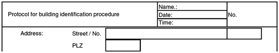

  

  Verifying and updating the building identification information

This is the first step in the whole procedure. Arriving at the site, the “identity” of the building must be first checked. Afterwards, the data collection can start: date, name and time are registered.

• (b) Walking around the building to identify its size and shape and looking for signs that identify the Construction year.

At first the building should be looked at to identify its size and shape and to get a first impression of the building. The construction year of a building can be determined if there is a sign at the facade of the building. If there is not such a sign, and the construction year cannot be determined, the field Construction Year is left empty (Fig. 8.5).

Fig. 8.5

Steps b, c and d

• (c) Determining and documenting occupancy.

This field describes the general usage of the building, like apartment building, school, kindergarten, hospital, office building, etc. If the building usage is not limited to one category the percentage of the usage categories are identified. Example: Apartments (70 %), Offices (30 %) (Fig. 8.5).

• (d) Determining the construction type.

The construction type can be difficult to identify in the field and without appropriate additional knowledge. However what can be determined easily is the construction material. Predominately this can be identified by visual inspection however the construction year can provide a good indication as construction materials (and construction types) have been largely used in specific historical periods. It can also be helpful to have a look into the building, if possible. Often the interior walls can give clues as to what building type is present. Sometimes it also helps to get into the basement, because the walls are not always covered in basements (Fig. 8.5).

• (e) Identifying the number of persons living/working in the building.

This step in the whole procedure allows estimating future casualties in case of an earthquake. To this aim, the number of occupants (living/working) of the building must be identified. The number of dwelling units can easily be determined in the entrance area of a building by looking at the number of door bells or the number of mail boxes. All dwelling units, even not used ones, should be counted. The next field addresses the number of people living or working in areas not depicted as dwelling units like shops at the basements, cafes, etc. The number can only be approximated, but this number should depict the maximum number of persons that can stay/work in the building. A practical example is the case of a building with a café on the ground floor and several dwelling units on the other floors. The maximum number of persons is given by the sum of the people leaving in the dwelling units (assessed as explained before) plus the maximum number of people that can occupy the café taking into account customers and employees (Fig. 8.7).

• (f) Characterizing the building through the ground plan and determining the distance to traffic area.

The characterization of the building through the ground plan can mostly be made with a plan of the city (Fig. 8.6). There are three questions to be addressed: Is the building a Corner Building? Are there any adjacent buildings? Does the building have a rectangular ground plan?

Fig. 8.6

Plan views of various building configurations showing plan irregularities; arrows indicate possible area of damage (FEMA 2002)

The distance to traffic area means the lowest distance between building and street. Parking areas and sidewalks do not count as traffic areas and should not be considered. The purpose of this distance is to know whether street can be blocked by building debris or not (Fig. 8.7).

Fig. 8.7

Steps e and f

• (g) Characterizing the building elevation; Using the laser telemeter to define building height; identifying soft stories or added attic space.

Number of floors, including the ground floor has to be registered considering carefully also the additional attic space. Attic space counts only if the housing area is more than 50 % of the ground floor area. Also building height (defined as the height from the top edge of the sidewalk to the beginning of the cornice) must be measured. The easiest way is by means of a laser – telemeter. A remark is added in case that the building height can be only approximately measured. If the building height cannot be directly measured; an “a posteriori” assessment can be performed: a measuring tape is put it to the wall of the building and a photo is taken. The building height can then be determined afterwards. The same procedure can also be done with balconies, etc.

The presence of shops or cafes at the ground floor, that might represent a soft story, is also evaluated. A soft story is a floor (does not have to be the ground floor) where most of the interior walls are missing due to the space needed. Soft stories perform poorly under seismic excitation (Fig. 8.8).

Fig. 8.8

Identifying soft stories and additional attic spaces

Additional attic space can often be determined by looking at the windows at the attic or due to the existence of balconies. Also added attic spaces, representing a vertical discontinuity, have poor seismic performances.

• (h) Identifying façade elements inclusively number of windows and doors.

Number of windows and doors at the façade facing the street and when possible also for the sides facing the courtyard are identified.

Evaluation of façade elements alias how detailed the façade design is, is also registered. Examples are given in the figures below (Fig. 8.9).

• (i) Determining non-structural members.

Chimneys represent another vertical discontinuity with poor seismic performances. When possible, they must be counted, otherwise this field is left open (Fig. 8.10).

Fig. 8.9

Identifying façade elements

Fig. 8.10

Example for a building with eight chimneys

Also all those façade elements that can fall off the building and on the street are registered. This includes sculptures, balconies, statues, etc. It is important to count all potentially hazardous elements on the façade: shop signs are also considered here (Fig. 8.11).

• (j) Determining the overall condition of the building.

This part focuses on the overall condition of the building. The main attributes are the presence of water leakage, damages to the roof and cracks in the walls. This mainly means the cracks in the walls. It is, when possible, distinguished between cracks on the outside layer of façade (that do not represent a structural problem and therefore are not counted) and cracks in the walls. If the crack is going diagonal it should be counted anyways (Fig. 8.12).

Fig. 8.11

Examples for non-structural members

Fig. 8.12

Examples of cracks

Also the presence of humidity and efflorescence (revealed by a change in the façade color) is registered (Fig. 8.13).

Fig. 8.13

Condition assessment

The estimation of damage at the roof level can be rather difficult. Nevertheless, the presence of humidity on the façade at the conjunction roof-upper floor is synonymous of possible roof damage. When the access to the building is possible, photos can document the degrade state. Damages at the roof can be very dangerous if not properly treated.

• (k) Noting irregularities/anomalies.

If there is anything out of the ordinary that is not explicitly in the checklist this is the place to write it down. If anything is written down here, it should always be documented with a photo if possible (Fig. 8.14).

• (l) Taking pictures with the digital camera.

A software program can modify pictures and combine them. The software is designed to reconstruct a coherent building out of your photographs. Note that since it is an automatic process, it can always lead to unexpected results. In order to avoid these degenerated cases, photos must be taken with care and following some guidelines. For each new reconstruction project focus must be put on only one building, or even only one façade (Fig. 8.15).

Fig. 8.14

Irregularities/anomalies and soft story

Fig. 8.15

Focus on one building for each reconstruction project

Having chosen the façade, a careful track must be planed (Fig. 8.16): pictures should be shut moving in approximately a half-circle around the façade Note that those coherent paths, with distance of about 1–3 steps between the shots, deliver best results.

Fig. 8.16

Plan the path in front of the building. Move around occludes

In order to obtain a coherent point-cloud of the object, the biggest possible part of the object (façade) should be kept in each photograph (Fig. 8.17).

Fig. 8.17

Always try to keep the whole façade in the view port of the camera

It is important to avoid delivering images difficult to distinguish: highly repetitive façade can confuse the software and produce mismatches. In general it is better to supply fewer images with good quality, than too many poor photos (Figs. 8.18 and 8.19).

Fig. 8.18

Façade with highly repetitive content. Making close-up photographs from two ends of such building will produce ambiguous result. This is the type of input to be avoided

Fig. 8.19

Unclear data: difficulties in distinguishing among the sides of the building

8.2.2 Building Identification Process – An Example

This section provides an example for the building identification process (Fig. 8.20). The following example describes a part of the process for the city of Vienna. The first thing to do is choosing an area of interest and collecting all information about the area that does not need field work: street plans, building plans, geology maps, etc. Once this information has been gathered the route of the screeners can be identified. If the buildings to be identified are selected, the screeners can begin to investigate the area. It has been shown that the best way to begin the process is to have a very detailed route and detailed plans for the field observations. The last step is transferring the information on the BIP Data Protocols into the relational electronic Building BIP Database. This requires that all photos are numbered (for reference purposes), and that additional fields (and tables) be added to the database for those attributes not originally included in the database. After arriving at the site the screeners observe the building as a whole and begin the process of gathering the information in the building identification protocol, starting with name, date, time, protocol number and the street address. The next step is to take photos of the building. This step can also be performed at the end of the screening process, after filling all the fields of the protocol. After determining the building usage, the construction year and the construction type are being determined. These two fields can also be left empty, in case that the construction year or type cannot be determined for sure. The next big block of fields is pretty easy to determine, number of persons/dwelling units, ground plan, elevation and façade. Non-structural members cannot always be determined properly like number of chimneys. The procedure is the same as for the construction year, if the number cannot be determined for sure, the field should be left empty. After determining the overall condition of the building there is a big field for irregularities. In each example there is an oriel starting at the first floor. This is written in this field and a photo is taken.

Fig. 8.20

Building identification protocol

8.3 Deterministic and Probabilistic Analysis, Inputs and Outputs

A deterministic and a probabilistic analysis were performed in the area of interest. The EQvis software is based on Mid-America Earthquake Center software tool MAEviz (MAE 2013) and adapted in SYNER-G as a platform for performing deterministic earthquake simulations as well as various other tools for pre and post processing of the input and output data. The SYNER-G prototype software for probabilistic analysis was integrated into the EQvis platform. In this way we could perform the probabilistic analysis and at the same time use the tools for pre and post processing of the input and output data available into EQvis. Hence, EQvis platform was improved adding the probabilistic analysis to the original deterministic one.

The case study here described represents an application and a validation of the functions of the EQvis platform.

It is noteworthy to clarify that the deterministic (performed with EQvis) and the probabilistic analyses (as developed in the SYNER-G project and implemented in the SYNER-G prototype software) differ on the resolution level of input and output data. In EQvis input and output data refer to every individual building: for every single building, the analysis requires data on the structural characteristics, number of occupants, proximity to the streets, etc. Accordingly, the software provides the assessment of the damage and of the casualties related to every single building.

In the SYNER-G prototype software instead, the buildings are grouped into zones (census tracts) and for each of those zones, the structural features of the buildings are statistically classified (Wen et al. 2003). Also the results of the calculation represent a statistical distribution inside the census tracts. Due to this difference in the resolution, although referring to the same area, input data of the deterministic and probabilistic analysis are not coincident. The following paragraphs present first the deterministic analysis and subsequently the probabilistic analysis.

The reason for choosing both of the analysis types is that decision makers can benefit from both of them. The probabilistic case gives them an overview of the general situation and a full consideration of system of systems and the “risk” of having a damaging earthquake together with the probabilistic values for the consequences.

The deterministic case can help in getting some concrete values on the damage expected for a given earthquake. The decision maker can for example choose a worst case scenario and see directly what the consequences will be. Another important usage of the deterministic case has been shown in a demonstration case in Hungary where immediately after an earthquake EQvis has been used as a management platform to steer the rescue process (Schäfer et al. 2013).

8.4 EQvis Deterministic Analysis: Input Data

EQvis is an advanced seismic loss assessment, and risk management software which is based on the Consequence-based Risk Management (CRM) methodology. CRM provides the philosophical and practical bond between the cause and effect of the disastrous event and mitigation options. It enables policy-makers and decision-makers to ultimately develop risk reduction strategies and implement mitigation actions (Schäfer et al. 2013; Mid-America Earthquake Center 2009). In EQvis, a wide range of user-defined parameters are introduced. The breadth of user-defined parameters enables emergency planners to model a virtually unlimited number of scenarios.

It has an open-source framework which employs the advanced workflow tools to provide a flexible and modular path (Clayberg and Rubel 2008). It can run over 50 analyses ranging from direct seismic impact assessment to the modeling of socioeconomic implications. It provides 2D and 3D mapped visualizations of source and result data and it provides tables, charts, graphs and printable reports for result data. It is designed to be quickly and easily extensible (McAffer et al. 2010).

8.4.1 Input Data in EQvis

8.4.1.1 Building Data

The building data as collected with the procedure explained in the Sect. 8.2 is been added as attributes to shapefiles of the building footprints, which were created prior to the survey. Each building point gets an attribute table where the data of the survey is stored (Genctürk 2007; Genctürk et al. 2008). The next step is to ingest the data in the EQvis platform. The following figure shows the data in the platform which then serves as the basis for all analyses performed within the test case (Fig. 8.21).

Fig. 8.21

Buildings in the test area together with a small example of the attribute table

For what concerns the building structural damage, the EQvis user has to provide the inventory, the hazard characteristics, the fragility dataset (see Table 8.1), and the damage ratio dataset (see Sect. 8.5.2). These are the required information, though the user can provide some additional information to improve the result. For instance, in case required, also data concerning liquefaction could be added. This was not the case in Vienna, since the soil does not present liquefaction susceptibility.

Table 8.1 Fragility curves used in Vienna test case for RC and masonry buildings

8.4.1.2 Railway Data

As mentioned in the introduction, the Vienna railway network is a complex system consisting of many components. For a first attempt, in the deterministic analysis we considered only the most critical elements of the networks i.e. the railway tunnels and the railway bridges. The fragility functions used are listed in Table 8.2. The railway infrastructure is presented in Fig. 8.22.

Table 8.2 Fragility curves used in Vienna test case for the railway network

Fig. 8.22

Railway tunnels (top) and bridges (bottom) in the Brigittenau district

8.4.1.3 Road Network Data

The road network that crosses Brigittenau districts connects the north-east part of the city (the part that is located on the east side of the Danube) with the west side of the city that is also the neuralgic centre. Therefore the network consists of main roads (with four or more ways), road bridges that allow the connection east-west side of the river and additional small roads in the inner part of the district for internal displacements.

Table 8.3 shows the fragility functions used for the assessment roads bridges. In this test case, SYNER-G fragility functions have been used for the vulnerability assessment (Pitilakis et al. 2014).

Table 8.3 Fragility curves used in Vienna test case for the road network

Comparing Fig. 8.22 bottom with Fig. 8.23 bottom, we can note that some of the Danube bridges are only for railway network.

Fig. 8.23

The road bridges in the test area

8.5 EQvis Deterministic Analysis: Output Data

8.5.1 Seismic Hazard

Two deterministic cases were simulated: a 1950 historical earthquake located in Neulengbach with a moment magnitude of 6 and a “method testing” earthquake with a moment magnitude of 7. Table 8.4 gives the characteristics of the earthquakes produced for the simulations. Campbell and Bozorgnia (2006) NGA attenuation functions (Campbell and Bozorgnia 2006) are used.

Table 8.4 Earthquakes created for the simulations

In the framework of the SEISMID FP7 project, VCE has performed detailed studies on the soil characteristics in the Vienna basin. The result of the studies and measurements performed is a very detailed microzonation. In particular, very detailed results are available for the 20th districted where an extensive campaign of measurements was performed. The results are organized in the map in Fig. 8.24: two soil types (soil classes B and C) are identified according to EC 8 (CEN 2004).

Fig. 8.24

Soil types around the test area

8.5.2 Results

The 6.0 moment magnitude Neulengbach earthquake and the 7.0 moment magnitude earthquake produce different values of Peak Ground Acceleration and hence different damage scenarios.

We decided to display the damages scenarios in two different ways: for the Neulengbach earthquake, we considered the probability of reaching the damages state “slight”, which is the first damage state in the fragility curves used.

In the case of the “method testing” earthquake the “mean damage” as derived in Eq. 8.1 is considered.

$$ \mathit{meandamage}={g}_i* i+{g}_m* m+{g}_h* h+{g}_c* c$$

(8.1)

where i is the probability of reaching the damage state “slight”, m is the probability of reaching the damage state “moderate”, h is the probability of reaching the damage state “heavy” and c is the probability of reaching the damage state “complete”. The factors before the probabilities are called “damage ratios” and can be specified by the user when ingesting the data. The damage ratios used in this test case are written in Table 8.5.

Table 8.5 Damage ratios used in the test case

8.5.3 Results for the 7.0 Magnitude “Method Testing” Earthquake

EQvis computes and visualises the damage scenario at a very high resolution i.e. at building scale. The user can quickly look at the results for each building and filter them. Each building is characterized by a very detailed description of the contents as described in the previous chapters.

The distribution of damage to the buildings shows that the building stock is very homogenous (Fig. 8.25). There are very few building collapses, some heavily damaged buildings but the majority of the building stock remains in good condition.

Fig. 8.25

Building damage for the “method testing” earthquake

The damage to the railway tunnels is very low compared to the building damage (Fig. 8.26). There is only one tunnel with a mean damage of 0.05, a very low level. It was expected that an earthquake of this magnitude and distance will not produce major damages to tunnels in general.

Fig. 8.26

Railway tunnel (left) and railway bridge (right) damage for the “method testing” earthquake

The maximum mean damage to railway bridges is 0.11 which assumes certain relevance. As expected the bridges closer to the epicentre as well as the bridges with poor soil conditions have the highest values of damage.

The damage to road bridges is similar to the damages to the railway bridges (Fig. 8.27). As before, the mean damage increases towards southeast.

Fig. 8.27

Road bridge (right) damage for the “method testing” earthquake

8.5.4 Results for the “Neulengbach” Earthquake

This case reproduces an actual earthquake that occurred in 1590. There are very few articles and data about the consequences of this earthquake, but damages to some building in Vienna were reported in the historical annals.

The simulation confirms cases of potential failure for some buildings. The maximum mean damage is around 0.14 with moderate damage probabilities up to 0.34 (Fig. 8.28).

Fig. 8.28

Building damage for the “Neulengbach” earthquake

The damages to road bridges, railway bridges and tunnels are very low. (Figs. 8.29 and 8.30) All the figures show the probability of reaching the damage state “slight” and the maximum value is 0.18.

Fig. 8.29

Railway tunnel (left) and bridge (right) damage for the “Neulengbach” earthquake

Fig. 8.30

Road bridge damage for the “Neulengbach” earthquake

8.5.5 Probabilistic Analysis with the SYNER-G Prototype Software: Input Data

The SYNER-G prototype software allows performing of probabilistic analysis: hazard characteristics, buildings inventory, water supply system and road and electric power network are the required input. The probabilistic analysis is based on the Monte Carlo method, selecting a minimum value for the covariance of 0.02 and performing 10,000 runs. Each run is characterized by a different location and intensity of the earthquake, producing consequently different scenarios of damage (Duenas-Osorio 2005).

8.5.5.1 Seismic Hazard

For the seismic hazard input, two seismic zones with M_min = 5.5 and M_max = 7.5 are selected based on the results of the SHARE European research project (Giardini et al. 2013). Figure 8.31 shows the active seismic zones that could affect the Vienna site.

Fig. 8.31

Seismic zones that could affect Vienna site based on the SHARE results (Giardini et al. 2013)

We used Akkar and Bommer (2010) ground motion prediction equation, choosing the peak ground acceleration as primary Intensity Measure and area fault as source model. Expected values of magnitude can vary in the interval 4.8–6.2, according to the historical seismicity of the zone.

8.5.5.2 Buildings

Brigitttenau district has been divided into two land use zones, one in the north and one in the south. Three main sub-city districts are also identified: for each of them, general information concerning the buildings and their inhabitants (as respectively average building height and employment rate) are given as input.

In addition, 11 census tracts have also been identified (see Fig. 8.32). While in the deterministic analysis performed with EQvis, buildings have been input one by one, each one with its own characteristics, in probabilistic analysis, the buildings have been grouped into zones (census tracts) and for each of those zones, the structural features of the buildings have been statistically classified (Wen et al. 2003).

Fig. 8.32

Masonry and reinforced concrete buildings distribution in Brigittenau districts and sub-districts (red are the reinforced concrete buildings, blue the masonry buildings)

From the statistical analysis, it was determined that 70 % of the buildings in the district are masonry buildings, the remaining 30 % are reinforced concrete ones. All the sub-districts have a preponderance of masonry buildings; only in the 5th sub-districts the percentage of reinforced concrete buildings is greater than the one of masonry buildings.

Then, for each building typology, the more appropriate fragility curve has been selected (Table 8.3).

The final input gives for each census tract the percentage of buildings associated to the fragility curve selected.

The most used fragility function of masonry building is the RISK-UE2003 – M12-HR-UNIGE Approach and RISK-UE2003 – RC Moment Frame – MR-HC-IZIIS Approach for reinforced concrete structures.

8.5.5.3 Road Network

Figure 8.33 represents the road network (RDN) in Brigittenau district. Two main roads cut the district in the north-south direction (Jägerstraße and Brigittenauer Lände in the western side, along the Donau Kanal). Wallensteinstraße links the east side (where also a freight harbor is) to the west side of the city through the Friedensbrücke over the Donau Kanal.

Fig. 8.33

Road network in Brigittenau

Each node of the RDN is defined by its longitude and latitude; each side by its starting and ending nodes. From a functional point of view, starting and ending nodes on the north-south and east-west directions are defined as external nodes; the nodes where the main roads intersect are CBD-TAZ (Central Business District – Traffic Analysis Zones) type nodes; all the other are simple intersection nodes. All nodes are considered as not-vulnerable. Road sides are divided in principal (around 1,000 vehicles per hour) and minor (600 vehicles per hour). Principal roads are classified as major arterials; among the minor roads, we distinguished the primary collectors (those directly linking the major arterials to the smallest roads) and the secondary collectors (the viability of which in case of extensive collapses would not strongly affect the viability of other roads). The majority of road sides have two traffic lanes (roadsegmentA); Brigittenauer Lände has four traffic lanes (therefore considered as a roadsegmentB). All the sides are considered as vulnerable.

For each road it is also given its width, the distance with the adjacent buildings, specifying also if there are buildings on both sides or only on one side. The site characterization is expressed in terms of V_s30 values (at nodes and sides) and site class.

Neither tunnel, nor bridge is in the part of the district analysed.

8.5.5.4 Water Supply System

Figure 8.34 (left) represents the Water Supply System (in orange) overlaid to the Road Network: the Water Supply System mostly follows the Road Network (with some exceptions). Three external points (one on the north, one on the west and one on the south-east) represent the constanttank nodes that supply the water to the entire district. No vulnerability is assigned to the nodes, while all sides are considered vulnerable.

Fig. 8.34

Water supply system (left) and electric power network (right) overlying to the road network

Sides that deliver the water from the supply-nodes have bigger pipes diameter (1,200 mm); the other sides have smaller diameter (600 mm). Only 2 diameter sizes are present. All the pipes are in castIron and lay 2 m under the ground level. Also here, the site characterization is expressed in terms of V_s30 values (at nodes and sides) and site class. The fragility functions of ALA (2001) are used for the vulnerability analysis of pipelines.

Due to the configuration of the tested area (an island in a biggest context that is the whole city of Vienna), redundancy and interdependency of the water supply system as well as the electric power network (see next paragraph) as here reproduced for the probabilistic calculation are not fully represented. This affects the correctness of the results, at least from a quantitatively point of view.

8.5.5.5 Electric Power Network

The Electric Power Network follows the layout of the Water Supply System (Fig. 8.34 right). Two generator nodes are identified: one on the west side of the district where the thermal waste treatment plant of Spittelau is; the other one on the east side. The network lay underground and has a voltage of 230 kV. Also here, the site characterization is expressed in terms of V_s30 values (at nodes and sides) and site class.

For the vulnerability analysis of the electric power transmission stations, the fragility curves proposed in the SRM-LIFE (2007) research project are used, which are provided in terms of peak ground acceleration (PGA). The fragility curves for transmission substations are classified in three classes (open, mixed and closed-type).

Two set of 10,000 runs have been performed: the first simulation considers interdependency among electric power network and water supply system, the second instead considers the two systems not dependent from the other (Bompard et al. 2011).

8.5.6 Probabilistic Analysis with the SYNER-G Prototype Software: Output Data

8.5.6.1 Average Results

In the output of the probabilistic calculation the case study area is subdivided into cells and calculations are performed for each cell. Cell dimension is approximately 100 × 100 m. The results reported below refer to the case which interdependency is considered among the water supply system and the electric power network. In particular in what follows we report the data obtained by averaging the results of each run over the total number of runs. This implies that damage level (for buildings, roads, water supply system, and electric power network) spans in the range 0–1, while deaths and injured average (being obtained as sum of affected persons divided by 10,000) can have a different range. Please note that the range in all of the figures can have a different meaning. It is always explained in the figure captions.

8.5.6.2 Buildings

Figures 8.35 and 8.36 present respectively the damage distribution and the affected persons in the area of interest. Biggest damage level and death/injured persons are mainly concentrated in the south zone of the district where there are almost only masonry buildings.

Fig. 8.35

Average building collapse (left) and building yielding distribution (right): higher values correspond to more extend level of collapse/yielding

Fig. 8.36

Average death (left) and injured (right) distribution

Analyzing the mean annual frequency of exceedance and the moving average (Fig. 8.37) one can obtain:

Fig. 8.37

Mean annual frequency of exceedance and moving average (death persons)

• Mean annual frequency of exceedance – deaths – 500 years return period:

• 0.7 * 10⁻³ * 35,402 (inhabitants) = 24 (dead persons)

• Moving average – deaths – average over all runs:

• 1.1 * 10⁻⁴ * 35,402 (inhabitants) = 4 (dead persons)

The earthquake that corresponds to death toll with 500 years return period determines expected fatalities of 24 while over 10,000 runs average death persons tends to the value of 4.

Also, with reference to Fig. 8.38 one can obtain:

Fig. 8.38

Mean annual frequency of exceedance and moving average (injured persons)

• Mean annual frequency of exceedance – injured persons – 500 years return period:

• 1.9 * 10⁻³ * 35,402 (inhabitants) = 67 (injured persons)

• Moving average – injured persons – average over all runs:

• 3 * 10⁻⁴ * 35,402 (inhabitants) = 11 (injured persons)

8.5.6.3 Roads

Analysing the roads damage, we obtain that blocked roads are mainly concentrated in the proximity of collapsed buildings (Fig. 8.39). In particular, this applies for small roads where the debris of collapsed buildings can partially or totally block the access of the adjacent roads.

Fig. 8.39

Average blocked roads. Darkest lines represent lower level of usability

8.5.6.4 Water Supply System

Pipes and nodes of the water supply system results to be slightly affected from the earthquake and average level of damage is negligible (Fig. 8.40). The obtained result is in agreement with what observed after real earthquakes: usually only at very high magnitude the water network has registered a significant level of damage.

Fig. 8.40

Pipes broken (left) and non-functional nodes (right). The damage is completely negligible

8.5.6.5 Electric Power Network

Also the electric power network results to be slightly damaged as shown in Fig. 8.41. There is almost no damage to the electric power network.

Fig. 8.41

Average damage on the electric power network nodes

8.5.7 Selected Scenario

Among the 10,000 runs, a particular scenario has been selected. It presents a 5.4 magnitude earthquake located in the south-east of Vienna, at a distance of approximately 50 km from Brigittenau district (Fig. 8.42). The selected scenario is considered meaningful since it is in the proximity of the tectonic zone of the Austrian region more prone to seismicity.

Fig. 8.42

M = 5.4 earthquake 50 km far from Brigittenau district, south-east of Vienna

This scenario produces a PGA distribution that can reach values of 0.4 m/s². For the sake of simplicity, those values refer to hard rock; soil typology in each point of the calculation should be considered in order to obtain the real soil acceleration.

8.5.7.1 Buildings

Figures 8.43 and 8.44 present respectively the distribution of collapsed and yield buildings, death and injured persons and displaced persons in case of good and bad weather conditions.

Fig. 8.43

Number of buildings collapsed (left) and yield (right) for the selected event of M = 5.4

Fig. 8.44

Number of deaths (left) and injured (right) persons for the selected event of M = 5.4

Comparing damage level and casualties, we obtain a higher number of deaths in correspondence to the collapsed buildings as it could be expected. Major damage is registered, as in the averaged results, in the south of the district where mainly masonry buildings are.

Figure 8.45 shows the distribution of displaced persons: the main difference among the case of bad weather and good weather is that in the first case there is an increment of the number of displaced persons in the north part of the district where reinforced concrete buildings are mainly located.

Fig. 8.45

Number of displaced persons in case of bad weather (left) and good weather (right)

8.5.7.2 Roads

Figure 8.46 presents the damage distribution on the road network of Brigittenau district. As in Fig. 8.39, blocked roads are mainly located in the south of the district, in proximity to more vulnerable structures.

Fig. 8.46

Blocked roads left for the selected scenario

8.5.7.3 Water Supply System

The selected scenario does not produce any damage to the water supply system. This is expected considering that the average damage level obtained before was negligible.

8.5.7.4 Electric Power Network

Finally, Fig. 8.47 presents the damage level that affects the electric power network.

Fig. 8.47

Damage level on the electric power network for the selected scenario

Table 8.6 reports the summary of damage caused by the selected event.

Table 8.6 Data from the selected event

8.6 Conclusions

The Vienna test case within the SYNER-G project has brought a proof of concept and provided a number of interesting lessons. It has been proven that an assessment process at the building level is feasible with the methods developed in SYNER-G. It turned out to be sufficient to have untrained personnel performing the large data gathering exercise using the BIP. This will help implementation on a very large scale and in any region of the world. IT tools are available to support the data collection and provide help to the involved forces.

The application of the methodology to a limited area with very detailed information provides a challenge for both the software application as well as the data collection: considering the limited area means missing redundancy in particular for what concerns the network system; very detailed scale implies to collect and to handle a large amount of data and information.

Both IT tools, namely the prototype software developed in SYNER-G for the probabilistic analysis and the EQvis platform, have been applied. The probabilistic analysis accounts the systemic interdependencies whereas EQvis is able to allow a user-friendly in and output of results. Visualization plays a major role when stakeholders and officials engaged in civil protection enter the procedures. The EQvis software platform with the integrated probabilistic SYNER-G software is available as an open-source product for free download at the homepage (www.syner-g.eu).

Different earthquake scenarios have been simulated. A plausibility check on the results obtained has been performed and it has been stated that they match with the expectations of the expert community. The results in terms of buildings are rated excellent whereas the results on the utility networks are limited because of the small area involved that does not allow to fully accounting for the interdependencies and the redundancies.

The two different approaches of the software tools, namely the deterministic and the probabilistic approach, can be used together in order to help decision makers make decisions. A general overview and a full consideration of system of systems of the situation can be given by the probabilistic approach while the deterministic approach can be used as a concrete scenario and eventually as a management platform during a crisis situation.

It will be a challenge to enlarge the dataset to the entire city (180,000 buildings instead of 700 in the test area). It will bring new challenges in terms of computing power and number of interrelations to be handled. Furthermore, from the experience gathered during the SYNER-G proof of concept, it is recommended to produce an online data generation sheet to allow filling the database with the necessary information. In order to perform this exercise it will be necessary to establish a large IT project that enlarges the current boundaries of application.

References

Achs G et al (2010) Erdbeben im Wiener Becken. VCE, Wien
Akkar S, Bommer JJ (2010) Empirical equations for the prediction of PGA, PGV and spectral accelerations in Europe, the Mediterranean Region, and the Middle East. Seismol Res Lett 81(2):195–206
ALA (2001) Seismic fragility formulations for water systems. American Lifeline Alliance, ASCE
Bompard E, Wu D, Xue F (2011) Structural vulnerability of power systems: a topological approach. Electr Power Syst Res 81(7):1334–1340
Borzi B, Pinho R, Crowley H (2007) SP-BELA: un metodo meccanico per la definizione della vulnerabilità basato su analisi pushover semplificate, ANIDIS, Pisa (in italian)
Borzi B, Crowley H, Pinho R (2008) The influence of infill panels on vulnerability curves for RC buildings. In: Proceedings of the 14th world conference on earthquake engineering, Beijing, China
Campbell K, Bozorgnia Y (2006) Next generation attenuation (NGA) empirical ground motion models: can they be used in Europe? In: Proceedings of the first European conference on earthquake engineering and seismology, Geneva, 3–8 Sept 2006.
CEN (2004) Eurocode 8: design of structures for earthquake resistance
Clayberg E, Rubel D (2008) Eclipse plugins, 3rd edn. Addison Wesley, Upper Saddle River
Duenas-Osorio LA (2005) Interdependent response of networked systems to natural hazards and intentional disruptions. Dissertation, Georgia Institute of Technology
Erberik MA (2008) Fragility-based assessment of typical mid-rise and low-rise RC buildings in Turkey. Eng Struct 30(5):1360–1374
Erberik MA, Elnashai AS (2004) Vulnerability analysis of flat slab structures. In: 13th world conference on earthquake engineering, Vancouver
FEMA (2002) Rapid visual screening of buildings for potential seismic hazards, FEMA154, 2nd edn. Applied Technology Council, Redwood City
Flesch R (1993) Baudynamik band 1. Bauverlag, Wien
Genctürk B (2007) Improved fragility relationships for populations of buildings based on inelastic response. MS thesis, University of Illinois at Urbana-Champaign
Genctürk B, Elnashai AS, Song J (2008) Improved fragility relationships for populations of buildings based on inelastic response. In: Proceedings of the 14th world conference on earthquake engineering, Beijing, China, 12–17 Oct 2008
Giardini D, Woessner J, Danciu L, Crowley H, Cotton F, Grünthal G, Pinho R, Valensise G, Akkar S, Arvidsson R, Basili R, Cameelbeeck T, Campos-Costa A, Douglas J, Demircioglu MB, Erdik M, Fonseca J, Glavatovic B, Lindholm C, Makropoulos K, Meletti C, Musson R, Pitilakis K, Sesetyan K, Stromeyer D, Stucchi M, Rovida A (2013) Seismic Hazard Harmonization in Europe (SHARE). Online data resource, http://portal.share-eu.org:8080/jetspeed/portal/. doi:10.12686/SED-00000001-SHARE
Kappos AJ, Nuti C, Sucuoglu H (2003) Seismic assessment and retrofit of RC buildings: case studies. fib Bulletin No. 24, May 2003, pp 251–306
LESSLOSS (2005) LESSLOSS deliverable report D84 – report on building stock data and vulnerability data for each case study
MAE (2013) MAEviz, developed by the Mid-America Earthquake Center and the National Centre for Supercomputing Applications. http://mharp.ncsa.illinois.edu/
McAffer J, Lemieux JM, Aniszczyk C (2010) Eclipse rich client platform, 2nd edn. Addison Wesley, Upper Saddle River
Mid-America Earthquake Center (2009) Impact of new Madrid seismic zone earthquakes on the Central USA, MAE Center report no. 09-03
Pitilakis K, Crowley H, Kaynia A (eds) (2014) SYNER-G: typology definition and fragility functions for physical elements at seismic risk, vol 27, Geotechnical, geological and earthquake engineering. Springer, Dordrecht. ISBN 978-94-007-7871-9
RISK-UE (2003) An Advanced approach to earthquake risk scenarios with applications to different European towns. WP4: vulnerability of current buildings risk-UE 2003, Greece
Schäfer D, Pietsch M, Wenzel H (2013) EQvis: a consequence based risk management software tool. In: Proceedings of the 5th international conference on structural engineering, mechanics and computation, University of Cape Town, 2–4 Sept 2013
SRMLIFE (2007) Development of a global methodology for the vulnerability assessment and risk management of lifelines, infrastructures and critical facilities. Application to the metropolitan area of Thessaloniki. Research project, General Secretariat for Research and Technology, Greece
Vargas YF, Pujades LB, Barbat AH (2010) Probabilistic assessment of the global damage in reinforced concrete structures, 14ECEE, Ohrid
Wen YK, Ellingwood BE, Bracci J (2003) Vulnerability function derivation for consequence-based engineering. Mid-America Earthquake Center report
Acknowledgments
The authors would like to acknowledge all colleagues at VCE, especially Reinhard Scherer and Thomas Gruber, as well as all colleagues from the MAEviz team for their support.
Author information
Authors and Affiliations
Corresponding author
Editor information
Editors and Affiliations
Rights and permissions
Copyright information
© 2014 Springer Science+Business Media Dordrecht
About this chapter
Cite this chapter
Wenzel, H., Schäfer, D., Bosi, A. (2014). Application to the City of Vienna. In: Pitilakis, K., Franchin, P., Khazai, B., Wenzel, H. (eds) SYNER-G: Systemic Seismic Vulnerability and Risk Assessment of Complex Urban, Utility, Lifeline Systems and Critical Facilities. Geotechnical, Geological and Earthquake Engineering, vol 31. Springer, Dordrecht. https://doi.org/10.1007/978-94-017-8835-9_8
Download citation
DOI: https://doi.org/10.1007/978-94-017-8835-9_8
Published:
Publisher Name: Springer, Dordrecht
Print ISBN: 978-94-017-8834-2
Online ISBN: 978-94-017-8835-9
eBook Packages: Earth and Environmental ScienceEarth and Environmental Science (R0)