
Abstract
Concatenated Hazards refers to situations where one extreme event precipitates one or more other extreme events. The exemplar is the tsunami and the resulting nuclear accident that occurred in Japan following the 11 March 2011 magnitude 9 earthquake.
Australia’s major natural hazards are hydro-meteorological in nature and have resulted in concatenated hazard events. An example is the 2011 Cyclone Yasi. The rainfall in the Australian tropics is due to the effects of the monsoonal wet season, augmented by the extra rainfall from the occasional tropical cyclone. Though tropical cyclones themselves can produce strong winds, storm surges, and floods – the combination of a particularly wet wet-season and a tropical cyclone can intensify the disaster and amplify the consequences. This was the situation on 3 February 2011 when Cyclone Yasi made landfall in North Queensland, following on a December-January period that had seen extensive flooding in Queensland as a result of a strong La Nina. The extra concatenation from Tropical Cyclone Yasi was the increase in Australian banana prices.
The predictive ocean–atmosphere model (POAMA) of the Centre for Australian Weather and Climate Research indicated in May 2010 that the wet season in Queensland would be extensive, with large amounts of rainfall. Tropical cyclone Yasi, though intense, had a well-behaved track and from 30 January was forecast to make landfall in Northern Queensland.
Model results indicate that the effects of climate change will be to decrease the numbers of tropical cyclones affecting Northern Australia and to increase the proportion of severe tropical cyclones affecting the region.
The Australian Government’s right to retain a non-exclusive, royalty-free license in and to any copyright is acknowledged.
Access provided by Autonomous University of Puebla. Download chapter PDF
Keywords
14.1 Concatenated Hazards
Concatenated Hazards refers to situations where one extreme event precipitates one or more other extreme events. The exemplar is the tsunami and the resulting nuclear accident that occurred in Japan following the 11 March 2011 magnitude 9 earthquake.
This particular example was triggered by the magnitude Mw = 9.03 earthquake, known as the Great East Japan Earthquake, the Tohoku earthquake, or the Tohoku-Oki earthquake that occurred at 14:46 JST (UTC+9). This was the most powerful known earthquake to have occurred in the region of Japan and is one of the most powerful earthquakes to have occurred since modern seismic record-keeping.
Ide et al. (2011) estimate the fault plane of the earthquake to be 440 × 220 km and Simons et al. (2011) note that the distribution of co-seismic fault slip exceeded 50 m in several places. Such an earthquake, which leads to a vertical displacement of the ocean floor, will create a tsunami. This is well known, and the announcements of the Japan Meteorological Agency that issued the most serious warning on its scale, namely a “Major Tsunami Warning”, immediately after the 11 March earthquake probably saved many thousands of lives.
Thus at the simplest, and most well-known level, earthquakes and tsunamis are concatenated hazards. However, in the case of the 11 March earthquake, the size of the tsunami was of such unexpected magnitude that the tsunami proceeded to trigger other disasters. The Japan Meteorological Agency rates a major tsunami as one that is at least 3 m high. However, because local undersea topography and the shape of inlets and harbours can amplify incoming waves, the size of a tsunami wave that affects a community can vary greatly. It was estimated that the tsunami reached heights of up to 40.5 m in Miyako in Tohoku’s Iwate Prefecture.
The damage by surging water proved to be more deadly and destructive than the earthquake itself. The confirmed death toll in September 2012 was 15,878 of which at least 12,143 died by drowning. Although Japan has heavily invested in anti-tsunami sea walls that line at least 40 % of the coastline and stand up to 12 m high, the tsunami simply washed over the top of some seawalls, collapsing some in the process. This over-topping was captured on numerous video images and news documentaries that were shown in the immediate aftermath of the tsunami. It would appear (Heki 2011) that neither seismologists nor oceanographers had expected an earthquake of such magnitude or a tsunami of such magnitude.
Though it is well-known that fire is a consequence of earthquakes, and indeed the 11 March earthquake triggered fires at two oil refineries, the nuclear power stations were prepared for such an eventuality and automatically shut down following the earthquake. When a reactor has been shut down, cooling is needed to remove residual heat and to maintain spent fuel. The backup cooling process is normally powered by emergency diesel generators but at Fukushima tsunami waves overtopped seawalls and destroyed backup power systems. This led to severe overheating at Fukushima Dai-ichi resulting in three large explosions, the leakage of radioactive materials and the evacuation of over 200,000 people when the Japanese Government declared a state of emergency. Altogether six nuclear reactors developed problems with Fukushima Dai-ichi being the worst.Footnote 1
14.2 Australia
Though Australia is subject to intra-plate earthquakes, its major natural hazards are hydro-meteorological in nature and are capable of producing concatenated hazard events. An Australian poet characterised Australia as a land “of droughts and flooding rains”. The droughts make the countryside prone to wildfires, which are known in Australia as bushfires and the rains, as the poet emphasises, lead to floods.
The Centre for Australian Weather and Climate Research (CAWCR) is a partnership between the Australian Bureau of Meteorology and the Commonwealth Scientific and Industrial Research Organisation (CSIRO) Division of Marine and Atmospheric Research. CSIRO is the Australian Federal Government’s major research agency which means that the partnership offers the possibility of bringing both research and operational expertise to bear on issues related to weather and climate. One of the areas in which this partnership has borne fruit is in the treatment of floods and tropical cyclones in which the research base of CSIRO has combined with the forecasting arm of the Bureau of Meteorology to improve the service offered to the Australian public.
The Australian public is concerned both with the occurrence of tropical cyclones in the immediate future, and in the longer term future when it is possible that climatic change may affect the distribution, landfall location, and intensity of tropical cyclones. CAWCR, through its Climate Variability and Change Research Program has the largest group of climate scientists in Australia working together to look at seasonal prediction, climate change and climate variability.
The rainfall in the Australian tropics is due to the effects of the monsoonal wet season, augmented by the extra rainfall from the occasional tropical cyclone. Though tropical cyclones themselves can produce strong winds, storm surges, and floods – the combination of a particularly wet wet-season and a tropical cyclone can intensify the disaster and amplify the consequences.
This was the situation on 3 February 2011 when Cyclone Yasi made landfall in North Queensland, following on a December-January period that had seen extensive flooding in Queensland as a result of a strong La Nina. The predictive ocean–atmosphere model (POAMA) of CAWCR indicated in May 2010 that the wet season in Queensland would be extensive, with large amounts of rainfall. Tropical cyclone Yasi, though intense, had a well-behaved track and from 30 January was forecast to make landfall in Northern Queensland.
Model results, discussed in detail in the Climate Change and Downscaling section, indicate that the effects of climate change will be to decrease the numbers of tropical cyclones affecting Northern Australia and to increase the proportion of severe tropical cyclones affecting the region.
14.3 Tropical Cyclones
On 25 December 1974, Tropical Cyclone TracyFootnote 2 destroyed virtually all of the Northern Australian city of Darwin causing the deaths of 71 people (49 on land and 22 at sea) and the evacuation of 75 % of the city’s residents. This event shocked the Australian public and encouraged the serious scientific study of Australian tropical cyclones.
This was not the first time Darwin had been severely damaged by a tropical cyclone: In both January 1897 and March 1937 the city was badly damaged, but only after Tracy was more attention given to building codes and other social aspects of disaster planning. Darwin was rebuilt and is now a thriving city of 128,100 people as at June 2011.
The Bureau of MeteorologyFootnote 3 provides a database of past tropical cyclones, histories of tropical cyclones, and a library of individual cyclone reports. Australian Tropical CyclonesFootnote 4 are classified according to the modified Saffir-Simpson scale shown in Table 14.1, with Category 1 tropical cyclones having winds below 42 m/s but above 33 m/s, which is the minimum wind speed needed for a tropical storm to be classified as a tropical cyclone. Category 5 tropical cyclones are the most intense and will cause catastrophic damage to structures.
There are, on average, approximately 12 tropical cyclones per year that are identified as occurring within the Australian region. Of these about 40 % (~5) make landfall over the Australian continent. Tropical cyclones and tropical storms provide a large proportion of rainfall in tropical Australia that ranges from 40 % in tropical Queensland to 60 % in tropical Western Australia (Lavender and Abbs 2013). Tropical cyclone climatologies for Australia have been used to determine the tropical cyclone hazard.
Numerical weather prediction models have not, as yet, reached sufficiently fine resolution that they can predict the formation and subsequent strengthening and motion of a tropical cyclone. They are, however, able to identify tropical lows so that a sufficiently skilled forecaster is able to use such numerical weather prediction models, along with satellite photographs of tropical cyclone clouds that position the tropical cyclone, and thus use the two items of information to assist with forecasts of tropical cyclone tracks.
Once the tropical cyclone has made landfall, there are four particular impacts that need to be considered: strong winds; extreme rainfall; the flooding associated with the cumulative rainfall; and the short term rise of sea level (known as storm surge).
During the severe wet season of January-February 2011 the eastern coast of Australia was affected by three tropical cyclones. Severe Tropical Cyclone ZeliaFootnote 5 from 14 to 18 January 2011, Tropical Cyclone AnthonyFootnote 6 from 22 to 31 January 2011, and Severe Tropical Cyclone YasiFootnote 7 from 30 January to 3 February 2011. Figure 14.1 depicts the track of Severe Tropical Cyclone Yasi. The scale shows very destructive winds in red, destructive winds in pink, and gale force winds are shaded.

Forecast track of TC Yasi as at 4 am on 2 February 2011. An animated version of this is available at: http://www.bom.gov.au/cyclone/history/yasi.shtml#loops
14.4 Concatenated Hazards and Cyclone Yasi
Concatenated Hazards refers to situations where one extreme event precipitates one or more other extreme events. In the case of TC Yasi (Fig. 14.1), a major portion of the Australian banana crop was wiped out causing extreme spikes in the banana price (Fig. 14.2) – repeating the situation of 2006 when Tropical Cyclone Larry made landfall on 20 March 2006 and also destroyed 80–90 % of Australia’s banana crop. Australia is relatively free of banana pests and diseases, and therefore does not allow bananas to be imported. Bananas were in short supply throughout Australia for the remainder of both 2011 and 2006, which increased prices across the country by 400–500 %.

Graph of North Queensland Banana Price and Banana supply indicating the effects of Cyclone Larry in 2006 and Cyclone Yasi in 2011 (Reserve Bank of Australia 2011)
14.5 Floods
The term “flood” covers a large variety of different hydrological events that can range from local flooding due to a blocked drain or culvert; short-term flash flooding of creeks as a result of a heavy, but localised storm; to the long-term flooding that occurs as rivers over-top their banks and inundate the floodplain that surrounds them. The dramatic effects of localised severe storms and flash flooding were graphically illustrated in January 2011 when the continuation of heavy rainfall that had started over much of Queensland in December 2010 caused severe flash flooding in the centre of the City of Toowoomba.
The Flood Commission of Inquiry in its interim reportFootnote 8 states that:
On 10 January, the Gowrie Creek catchment experienced intense rainfall between 1.00 pm and 2.30 pm. In the city of Toowoomba itself, heavy rain began falling at about 12.45 pm, and peaked between 1.45 pm and 2.15 pm.
The most severe rain fell in a northeast - southwest band that covered the middle and lower parts of East and Westcreeks, where they crossed Toowoomba’s central business district 21. This concentration of rain in the East Creek and West Creek catchments continued for approximately 60 to 90 minutes. It had largely ceased between 2.15 pm and 2.45 pm.
The intense rainfall over the catchment of the three creeks caused a severe flash flood in the city between 1.30 pm and 2.45 pm. Closed circuit television footage provided by Toowoomba Regional Council shows water rising at extraordinary speed and flowing over the roadways. It also demonstrates the speed with which the water rose. It is clear that this was not a situation in which any agency could have effectively warned residents of what was to come.
Water covered all the roadway crossings of East, West and Gowrie Creeks, making them impassable to pedestrians and vehicles. The rapidity of the flooding caught people by surprise: in city streets they found themselves surrounded by water, or were trapped in their vehicles. A woman and her teenaged son lost their lives when their car was caught in the flooding in a city intersection. A number of buildings in and around the city were extensively damaged, and numerous parked cars were swept away or inundated by the flooding.
On the same day the Lockyer creek, in the Lockyer Valley to the east of Toowoomba flooded and residents suggest that flooding in the town of Grantham occurred between approximately 3.20 pm and 4.00 pm. The flood appeared as a wave, sweeping from the Lockyer Creek across the paddocks and through the town. Thirty-six people died in the 2010/2011 floods with an estimated reconstruction cost of $5 billion.
14.6 Seasonal Forecasting
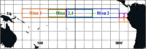
The Bureau of Meteorology has developed a seasonal prediction model known as POAMA, which is an acronym for the Predictive Ocean Atmosphere Model for Australia. It is a dynamic computer model of the climate system run on the operational super-computer that is used to generate weather forecasts. Because the weather and climate of the eastern part of Australia is strongly influenced by El Nino (McBride and Nicholls 1983), a significant product generated by POAMA consists of model forecasts of the El Niño - Southern Oscillation. They are provided as an operational product on the web site of the Bureau of Meteorology and are included in the monthly model summaryFootnote 9 of predictions from POAMA and other models operated by international organisations. Because the south-eastern Australian climate is also influenced by the Indian Ocean Dipole (IOD), forecasts of the IOD are also provided.Footnote 10
The latest operational version of POAMA is POAMA2 (version 2.4). A 30 member ensemble of POAMA-2 forecasts is run twice per month and gives forecasts out to 9 months ahead. Probabilities are based on a 30-member ensemble from POAMA-2 starting on the 1st and the 15th of the month. The results, which are forecast out to 9 months lead, show all the runs so that the probability distributions that result provide a range of possible developments in sea surface temperature (SST) in the equatorial Pacific OceanFootnote 11 and for the Indian Ocean. More detailed information about the model is available on the experimental POAMA page: http://poama.bom.gov.au/. Further details on POAMA 2 SST skill can be found in Wang et al. (2011). A separate system (POAMA-2 Multiweek) is now run every week in experimental mode to produce an ensemble of 33 members also out to 9 months. This system is tailored to forecasting on multi-week/monthly timescales and includes a new coupled breeding method.
The performance of the POAMA model is illustrated in Fig. 14.3 which depicts the Brier skill scoreFootnote 12 for POAMA1.5, POAMA 2.4, a re-calibrated version of POAMA2.4, and a five member multi-model ensemble that incorporates POAMA 2.4a, POAMA 2.4b, POAMA 2.4c plus ECSys3 (Stockdale et al 2011) and the UKMO HadGEM2 seasonal forecast (Arribas et al 2011) initialised on 1 May 2010 for the October-December 2011 forecast. Details of skill over Australia, including a comparison with other international models can be found in Langford and Hendon (2011).

Australian rainfall Brier skill score for POAMA1.5 (p15b), POAMA 2.4 (P24 MME), a re-calibrated version of POAMA2.4 (P24 cal MME), and a five member multi-model ensemble that incorporates POAMA 2.4a, POAMA 2.4b, POAMA 2.4c plus ECSys3 and the UKMO HadGEM2 seasonal forecast (5 model MME) initialised on 1 May 2010 for the October-December 2011 forecast
14.7 POAMA and the Beijing Floods of 21 July 2012
On Saturday 21 July 2012 Beijing suffered the heaviest rainfall for over 60 years with the average precipitation reaching 170 mm, while a town in the suburban district of Fangshan, received 460 mm of rain. The storm was widespread. In Hebei province as at 26 July 2012, 32 people were confirmed dead and another 20 missing after the storm over the weekend. More than 2.66 million people had been directly affected by the storm that flooded 59 counties in Hebei province. The official death toll until 27 July was reported as 37 people after which it was raised to 77 people. Direct economic losses totalled more than 12.28 billion yuan ($1.92 billion).
Using archived POAMA output, we have examined (Fig. 14.4) the performance of POAMA in being able to forecast high rainfall in the Beijing area. POAMA consistently provided forecasts of high rainfall (exceeding 10 mm/day) for the Beijing region as from 28 June 2012 indicating that there was approximately 3 week predictability for this event from a seasonal prediction model. The Bureau of Meteorology numerical weather prediction model, called ACCESS, was able to provide high resolution analysis 48 h before the storm that indicated that localised precipitation in excess of 100 mm/day was to be expected.

POAMA forecast made on 28 June 2012 predicted heavy rainfall in the Beijing area for the 12 July–25 July 2012 period
14.8 May 2010 POAMA Forecast
Figure 14.5 depicts the observed (green curve) and the ensemble of POAMA2.4 forecasts indicated by the dark green curve and the shading around it for the Nino34 SST index during 2010 and early 2011. The forecasts were initialized on 1 May 2010. The strong La Niña during 2010, which contributed to extreme rainfall in eastern Australia during spring and early summer, was not predictable prior to May 2010, but by May 2010 the POAMA2.4 forecasts were clearly indicating the development of a strong cold event that would extend for at least the next 9 months.

May 2010 forecasts of the El Nino index from POAMA indicating that strong La Nina conditions were to be expected at least the next 9 months. La Nina conditions are indicative of above normal rainfall in Eastern Australia
POAMA also provides information on the spatial distribution of expected rainfall. Figure 14.6 shows the observed (Fig. 14.6a) and forecast (Fig. 14.6b) rainfall anomaly for October-December 2011 for Australia. The forecast is the 30 member ensemble mean from the POAMA2.4 seasonal forecast that was initialized on 1 May 2010. The color bars are the same for Fig. 14.6a, b. Extreme wet conditions in eastern Australia for October-December 2011 were well forecast from at least 1 May 2010 due to the development of a strong La Niña event that was well predicted by the POAMA2.4 model, as shown in Fig. 14.6b.

(a) Observed rainfall anomalies for October to December 2011. (b) POAMA Forecast of rainfall anomalies for October to December 2011
In fact this forecast was very accurate with extreme rainfall occurring over much of Eastern Australia. The dramatic effects of localised severe storms and flash flooding on topography that had been previously moistened was graphically illustrated in January 2011 when the continuation of heavy rainfall that had started over much of Queensland in December 2010 caused severe flash flooding in the centre of the City of Toowoomba.Footnote 13
The record rainfalls and flooding experienced across much of the region, and throughout Australia, in the 2010/11 and 2011/12 summers highlighted that the tropical Pacific ocean temperatures are not the only sea surface temperatures of importance but one needs to consider the status of all three oceans surrounding Australia – Pacific, Indian and Southern – in influencing seasonal and inter-annual rainfall variability. The spring/summer of 2010/11 saw one of the strongest La Niña events on record combined with a negative IOD event and a positive Southern Annular Mode (SAM) – i.e. all three key influences were in their wet phases in terms of expected rainfall impacts on south-eastern Australia.
SAM describes the north–south movement of the westerly wind belt that circles Antarctica, dominating the middle to higher latitudes of the Southern Hemisphere. The changing position of this westerly wind belt influences the strength and position of cold fronts and mid-latitude storm systems, and is an important driver of rainfall variability in southern Australia. In a positive SAM event, the belt of strong westerly winds contracts towards Antarctica. This results in weaker than normal westerly winds and higher pressures over southern Australia, restricting the penetration of cold fronts inland. The positive phase of SAM is typically associated with wetter and cooler conditions over much of Australia during spring and summer but with drier and cooler conditions over the southwest and southeast coasts of the continent during winter (Hendon et al. 2007).
These conditions, coupled with the warmest sea-surface temperatures on record to the north of the Australian continent, contributed to making 2010–11 Australia’s wettest two-year period on record. While the extensive flooding of 2010/11 was, by and large, consistent with natural variability, it is possible that ongoing global warming contributed to the magnitude of the event through its impact on ocean temperatures. The spring and summer of 2011/12 saw the re-emergence of another (weaker) La Niña event, combined with a positive SAM during early summer, but this time the Indian Ocean played a lesser role.
14.9 Climate Change and Downscaling
A question of continuing relevance relates to the influence of climate change on tropical cyclone numbers, intensity and landfall location. Callaghan and Power (2011) examined the statistics of past Queensland tropical cyclones and found that the number of tropical cyclones making landfall over eastern Australia declined from about 0.45 TCs/year in the early 1870s to about 0.17 TCs/year in recent times. They noted that this decline can be partially explained by a weakening of the Walker Circulation, and a natural shift towards a more El Nino-dominated era. The extent to which global warming might be also be partially responsible for the decline in land-falls – if it is at all – is unknown.
This question has been examined by using dynamical downscaling of computer models (Daloz et al. 2012). In particular the output from the 200 km resolution CSIRO Mark 3.6 general circulation model has been nested into the 65 km output of CCAM in which tropical cyclone-like vortices are detected. The details of these vortices are then elucidated using mesoscale models such as RAMS and WRF that have 5 km resolution. Using this method, simulations were undertaken for the present climate and for the end of the twenty-first century using the SRES A2 scenario. Based on 11 simulations there is a strong signal confirming a decrease in tropical cyclone numbers in the Australasian region – both north-eastern Australia and north-western Australia.
The maximum wind speed of tropical cyclones increases from about 32 m/s to about 37 m/s and associated with this increase in maximum wind speed there is a marked increase in the maximum integrated kinetic energy of tropical cyclones. At the moment the probability distribution of maximum integrated kinetic energy has a mode (consisting of 16 % of tropical cyclones) at 55 TJ. This mode lies at 75 TJ in the simulations for 2070. The radius of maximum winds is also increased from 90 km at present to 130 km in 2070.
Table 14.2 depicts the changes in precipitation between the situation in 2010 and the situation in 2070 at various distances from the centre of the tropical cyclone. In all cases except one both the average rainfall intensity and the maximum rainfall intensity increases. The exception is the average rainfall at 100 km from the centre of the tropical cyclone which decreases by 9 %. These results are all consistent with the concept that under climate change tropical cyclones will increase in size and be stronger.
The projected changes between 2010 and 2070 in the number, duration and location of Australian tropical cyclones obtained by downscaling seven general circulation models is shown in Table 14.3.
The models are all consistent in indicating that the number of tropical cyclones will decrease. Though the occasional model may produce different results there is also an overwhelming consensus that the duration of tropical cyclones will decrease – though all models appear to indicate overly short duration times. There is also a consensus that tropical cyclones move equatorward – both in terms of the location of their genesis, and the location of their decay (which, presumably, approximates to their landfall). These results apply both to tropical cyclones in the south western Pacific Ocean, which are the ones that affect Queensland on the east coast of Australia, and to tropical cyclones in the southern Indian Ocean, which are the ones that affect Western Australia.
14.10 Summary and Conclusion
Advances in numerical weather prediction, combined with information on the drivers of Australian climate have led to the production of a seasonal forecasting model, known as POAMA, that has displayed considerable skill in the production of multi-week and seasonal forecasts. POAMA could have been used to provide about 3 weeks warning of the 21 July 2012 heavy precipitation in Beijing.
POAMA was also successful in its May 2010 predictions of the La Nina that led to extreme rainfall in eastern Australia during the last quarter of 2010 and the first quarter of 2011. Both the magnitude and spatial extent of the rainfall were accurately reproduced. This time period corresponded to extreme flash flooding in parts of Queensland, and flooding in Brisbane, the capital of Queensland. During a La Nina event, there is a tendency for tropical cyclone numbers to increase – and there were three tropical cyclones that made landfall in Queensland over this period. Cyclone Yasi, the most memorable, destroyed the Queensland banana crop.
By using dynamical downscaling techniques it is possible to use general circulation models to investigate the impact of climate change on the likely changes in tropical cyclone numbers, intensity, duration and location.
Climate change models are all consistent in indicating that the number of tropical cyclones will decrease (Abbs 2012) such that on average for the period 2051–2090 there will be an approximately 50 % decrease compared to the 1971–2000 period. There is also an overwhelming consensus that the duration of Australian tropical cyclones will decrease – though all models appear to indicate overly short duration times. There is also a consensus that Australian tropical cyclones move equatorward – both in terms of the location of their genesis, and the location of their decay (which, presumably, approximates to their landfall).
The POAMA and other seasonal forecast models, as well as climate change models – especially downscaled general circulation models - could provide predictions of the likelihood of concatenated hazards such as tropical cyclones and agricultural losses or severe storms and flash floods. This knowledge could be used to prepare for and reduce the effects of these types of hazards.
Notes
- 1.
- 2.
- 3.
- 4.
- 5.
- 6.
- 7.
- 8.
- 9.
- 10.
- 11.
- 12.
- 13.
References
Abbs D (2012) The impact of climate change on the climatology of tropical cyclones in the Australian region. CSIRO Climate Adaptation Flagship Working Paper No. 11. http://www.csiro.au/en/Organisation-Structure/Flagships/Climate-Adaptation-Flagship/CAF-working-papers.aspx
Arribas A et al (2011) The GloSea4 ensemble prediction system for seasonal forecasting. Mon Weather Rev 139:1891–1910
Callaghan J, Power SB (2011) Variability and decline in the number of severe tropical cyclones making land-fall over eastern Australia since the late nineteenth century. Clim Dyn 37:647–662. doi:10.1007/s00382-010-0883-2
Daloz AS, Chauvin F, Walsh K, Lavender S, Abbs D, Roux F (2012) The ability of general circulation models to simulate tropical cyclones and their precursors over the north Atlantic main development region. Climate Dynam 39:1559–1576. doi:10.1007/s00382-012-1290-7
Heki K (2011) A tale of two earthquakes. Science 332(6036):1390–1391
Hendon H, Thompson DWJ, Wheeler MC (2007) Australian rainfall and surface temperature variations associated with the Southern Hemisphere annular mode, J. Clim., 20:2452–2467
Ide S, Baltay A, Beroza GC (2011) Shallow dynamic overshoot and energetic deep rupture in the 2011 Mw 9.0 Tohoku-Oki earthquake. Science 332(6036):1426–1429
Langford S, Hendon H (2011) Assessment of international seasonal rainfall forecasts for Australia and the benefit of multi-model ensembles for improving reliability. CAWCR Technical Report No. 039
Lavender SL, Abbs DJ (2013) Trends in Australian rainfall: Contribution of tropical cyclones and closed lows, Clime Dynam 40:317–326. doi:10.1007/s00382-012-1566-y
McBride JL, Nicholls N (1983) Seasonal relationships between Australian rainfall and the Southern oscillation. Mon Weather Rev 111:1998–2004
Reserve Bank of Australia (2011) Statement on Monetary Policy – Box B: An update on the impact of the natural disasters in Queensland, Reserve Bank of Australia, Sydney, May 2011
Simons M, Minson SE, Sladen A, Ortega F, Jiang J, Owen SE, Meng L, Ampuero JP, Wei S, Chu R (2011) The 2011 magnitude 9.0 Tohoku-Oki earthquake: mosaicking the megathrust from seconds to centuries. Science 332(6036):1421–1425
Stockdale TN, Anderson DLT, Balmaseda MA, Doblas-Reyes F, Ferranti L, Mogensen K, Palmer TN, Molteni F, Vitart F (2011) ECMWF seasonal forecast system 3 and its prediction of sea surface temperature. Clim Dynam 37:455–471. doi:10.1007/s00382-010-0947-3
Wang G, Hudson D, Ying Y, Alves O, Hendon H, Langford S, Liu G, Tseitkin F (2011) POAMA-2 SST skill assessment and beyond. CAWCR Res Lett 6:40–46
Author information
Authors and Affiliations
Corresponding author
Editor information
Editors and Affiliations
Rights and permissions
Copyright information
© 2014 Springer Science+Business Media Dordrecht
About this chapter
Cite this chapter
Beer, T., Abbs, D., Alves, O. (2014). Concatenated Hazards: Tsunamis, Climate Change, Tropical Cyclones and Floods. In: Kontar, Y., Santiago-Fandiño, V., Takahashi, T. (eds) Tsunami Events and Lessons Learned. Advances in Natural and Technological Hazards Research, vol 35. Springer, Dordrecht. https://doi.org/10.1007/978-94-007-7269-4_14
Download citation
DOI: https://doi.org/10.1007/978-94-007-7269-4_14
Published:
Publisher Name: Springer, Dordrecht
Print ISBN: 978-94-007-7268-7
Online ISBN: 978-94-007-7269-4
eBook Packages: Earth and Environmental ScienceEarth and Environmental Science (R0)