Peculiarities of Water as an Environmental Habitat for Microorganisms

Abstract

As a habitat for the existence of microorganisms, water has properties not found in other natural microbial habitats such as soil, and plant and animal bodies; indigenous aquatic microorganisms are adapted to these conditions. Natural waters are generally low in nutrient content (i.e., they are oligotrophic); what nutrients there are, are homogeneously distributed in the water. The movement of water freely transports microorganisms; to counter this and offer themselves some protection, many aquatic organisms are either stalked or arranged in colonies immersed in gelatinous materials. To enable free movement in water, many aquatic microorganisms and/or their gametes have locomotory structures such as flagella. Microorganisms are often adapted to, and occupy particular habitats in the water body; some occupy the air–water interphase (neuston), while others live in the sediment of water bodies (benthic). The conditions which affect aquatic microorganisms are temperature, nutrient, light, salinity turbidity, water movement. The methods for the quantitative study of aquatic microorganisms are cultural methods (plate count and MPN), direct methods (micro­scopy and flow cytometry), and the determination of microbial mass. The microscopy methods are light (optical), epi-flourescence, confocal laser scanning microscopy, transmission electron microscopy, and scanning electron microscopy. Microbial mass may be direct (weight after oven-drying) or indirect (turbidity, CO₂ release, etc).

1 The Peculiar Nature of Water as an Environment for Microbial Habitation

Microorganisms exist in different natural environments such as the soil, the animal intestine, the air, and water. Each of these habitats has peculiar characteristics to which the organisms living therein must adapt.

Aquatic microorganisms generally experience highly fluctuating and highly varying environmental conditions. These conditions differ not only from one aquatic macro-environment to another, but also in diffe­rent sub-locations in the same aquatic macro-environment. This variability contributes to the well-recognized microbial biodiversity in aquatic environments. On account of this, because the freshwater macro-environment is clearly different from the marine macro-environment, the microorganisms attached to organic matter of the same composition would be expected to be different.

Various habitats can be recognized within an aquatic environment. Each habitat is characterized by one or more microbial communities.

This chapter will discuss the peculiarities of the aquatic environment as dwelling places for micro­organisms as well as the methods used in quantitative study of microorganisms found in water.

The aquatic environment can itself be divided broadly into freshwater and saline. The microbiology of the freshwater environment will be discussed in Chap. 5 and that of the saline (marine) environment in Chap. 6.

Water differs from other natural microbial environments such as soil, plant, and animal bodies in a number of ways, namely (Sigee 2005):

• 1. The low concentration of nutrients

  Natural bodies of water are generally oligotrophic, i.e., low in nutrients. The concentration of nutrients available to a microbial cell in the environment of natural waters such as the open sea or rivers away from shorelines is usually low, when compared with the concentrations found in other microbial habitats such as soil crevices or plant and animal bodies. The result of this is that the truly indigenous aquatic microorga­nisms must be able to subsist under conditions of low nutrient availability, which may be unfavorable to their terrestrial counterparts of the same group. For example, Escherichia coli is known to die out quickly in distilled water, whereas aquatic indigenes such as Pseudomomas spp. and Achromobacter spp. do not.

• 2. Relative homogeneity of the properties of water

  Because of the vastness of the aquatic environment in comparison with the size of the individual microbial cell, the aquatic environment is fairly homogeneous in terms of nutrients, pH, etc. For example, metabolic products released by aquatic microorganisms are continuously diluted away in natural waters, say in a river. Such pro­ducts, therefore, hardly accumulate in natural waters in the same way as they could theoretically do in the soil. Two samples of soils taken an inch apart from each other may have completely different properties in terms of pH, the population of microorganisms, etc. This is not the case with water which can be said to be more homogeneous both in space and time than other natural environments.

• 3. The movement of water

  Natural bodies of water generally flow. Even when there is no apparent gross movement of a body of water, minor movements induced by the wind take place regularly. Consequently, many truly aquatic microorganisms are attached to larger bodies which provide them with support, and stop them from drifting. In order to provide this attachment, some aquatic bacteria are stalked, for example, the aquatic bacterium Caulobacter spp. Others form filaments which enable attachment only at one end leaving the rest of the filament free for the absorption of nutrients. An example will be found among the adults of the sessile ciliated Protozoa such as those found among the Suctoria (see Chap. 4). Still others form themselves into gelatinous balls or masses which can offer slightly better protection against the hazards of moving waters than would be available to single individuals. Examples of orga­nisms which form colonial units or are immersed in gelatinous masses are Zooglea spp. among the Bacteria, and Pandorina spp. among the Algae.

  With respect to the terminology for describing water movements or flow of freshwaters, those which are still or exhibit little flow, e.g., ponds or some lakes, are known as limnetic waters, while those in which the movement or flow is rapid, as in some rivers and streams, are known as lotic.

• 4. Freedom of movement of microorganisms in aquatic environments

  Because of the vastness of the water environment in comparison with the size of microorganisms, aquatic microorganisms are afforded movement without impediment over comparatively huge distances in a way which is not available to organisms in soil or other environments inhabited by microorganisms. Most truly aquatic microorganisms possess flagella or cilia which enable them or their reproductive cells to move about freely in aquatic environments. This is presumably to help them move around freely in search of food or around those areas of the water body such as decomposing animal or plant bodies which may have slightly higher concentrations of nutrients than the rest of the water. In illustration of this, the truly aquatic fungi, i.e., Phycomycetes are the only group among the fungi in which flagellated gametes are found. Similarly, among the algae which are recognized as mostly aquatic, flagellated cells or reproductive structures are found in all of the algae except the Rhodophyceae (Red Algae) and the Cyanophyceae or Blue green algae.

2 Ecological Habitats of Microorganisms in Aquatic Environments

In the ecological study of plants and animals, a population is a group of living things of the same kind living in the same place at the same time, while a habitat is the place where a population lives (Pugnaire and Valladares 2007). These concepts are applied here to the microorganisms living in water. In aquatic environments, various, sometimes overlapping ecological populations of microorganisms exist at various depths of the water column. The various populations inhabi­ting various aquatic habitats will be described below (Matthews 1972):

• 1. Planktonic organisms

  Planktonic organisms are populations of free floa­ting organisms in water. They are the fodder (or food) upon which the smaller aquatic life, especially krills and small fish, subsist. Planktons include algae (Diatoms or Bacillariophyceae) and Dinoflagellates (Dinophy­ceae) as well as Protozoa.

• 2. Tectonic organisms

  In contrast to planktonic organisms, tectonic orga­nisms are those which, while subject to aquatic flow, also have locomotory means of their own, and hence can also move apart from being carried with the flow of water, e.g., ciliated protozoa, flagellated bacteria, etc.

• 3. “Aufwuchs” (periphyton)

  This is a term derived from the German; it indicates that the aquatic microorganism in question is attached to something. On the basis of the nature of their support, “aufwuchs” are divided into the following categories:

  • (a) Epiphytic – attached to the surfaces of plants

  • (b) Epizootic – attached to the surface of animals

  • (c) Epilithon – a community of microorganisms attached to rocks and stones of the aquatic environment

  • (d) Epixylon – the microorganisms found on the fallen woods in water bodies

  • (e) Episammon – the community of organisms attached to sand grains

• 4. Benthic organisms, benthos

  Organisms inhabiting the bottom sediment of aquatic environments (i.e., bottom or mud-dwelling organisms) constitute the benthic community or benthos.

• 5. Neuston

  The microorganisms which are found at the surface of an aquatic environment, exactly at the air–water interface, are referred to as neuston.

• 6. Pleuston

  The specific term “pleuston” may be used to denote the organisms occupying the air–water interface in a marine biota. These neuston and pleuston can be regarded as specialized communities as their air–water interface habitat is subjected to widely fluctuating environmental conditions.

• 7. Seston epipelon

  Sestons are the particulate matter suspended in bodies of water such as lakes and seas. Some authors apply it to all particulates, including plankton, organic detritus, and inorganic material. Seston produced by nekton, i.e., large swimming animals, may also act as a habitat along with other organic debris. Micro­organisms inhabiting these detritus matters and other fine sediment surface are referred to as epipelon.

3 Foreign Versus Indigenous Aquatic Bacteria

Microorganisms are constantly being washed into surface waters from the soil; thus the microbial population of the near-side of inland waters is very similar to the surrounding soil especially after rains. Those which are not truly indigenous to water soon die. These are the foreign, migrant, or allochthonous organisms of water, while the indigenous organisms, known as authochthonous, survive in the water (Fig. 2.1).

Fig. 2.1

Relative populations of allochthonous and authochthonous aquatic microorganisms after rainfall (Drawn by the author: see text)

4 Challenges of Aquatic Life: Factors Affecting the Microbial Population in Natural Waters

Various physical and chemical factors affect the microbial population in natural waters. The physical factors affecting the microbial populations in aquatic environments are floatation, temperature, nutrients, and light, while the chemical factors include nutrients, salinity, and pH (Sigee 2005).

• 1. Floatation

  Flotation or placement in the water column is a challenge faced by all aquatic organisms. For example, it is crucial to phytoplankton (microscopic algae) to stay in the photic zone, where there is access to sunlight. The small size of most phytoplankton, plus a special oily substance in the cytoplasm of cells, helps keep these organisms afloat.

  Zooplankton (microscopic protozoa) use a variety of techniques to stay close to the water surface. These include the secretion of oily or waxy substances, ­possession of air-filled sacs similar to the swim bladders of fish, and special appendages that assist in floating. Some zooplankton even tread water.

  Fishes have special swim bladders, which they fill with gas to lower their body density. By keeping their body at the same density as water, a state called “neutral buoyancy,” fishes are able to move freely up and down.

• 2. Temperature

  Temperature is one of the main factors affecting the growth of microorganisms. Psychrophiles (low temperature loving) are microorganisms which have an optimum temperature of growth of 0–5°C, whereas thermophiles (high temperature loving) have optimum temperatures of 60°C and above. Mesophiles (middle temperature loving) have optimum temperatures of 20–40°C. The temperature of natural waters varies from about 0°C in polar regions to 75–80°C in hot springs. In tropical regions it is about 25–30°C, and in temperate regions about 15°C in the summer and lower in the colder months.

  The specific thermal capacity of water is very high, hence large water bodies are able to either absorb or lose great amount of heat energy without much change in their temperature. Because of this, many aquatic organisms including microbes experience very stable temperature conditions. For instance, about 90% of the marine habitats maintain a constant temperature of about 4°C which encourages the growth of psychrophilic microorganisms. A good example of a marine psychrophile is Vibrio marinus, while a good example of a thermophile is Thermus aquaticus (optimum temperature 70–72°C) which grows in hot springs and whose thermostable DNA polymerase is used in the very useful procedure used to amplify DNA, the Polymerase Chain Reaction (PCR) see Chap. 3.

  The temperature of non-marine water bodies like lakes, streams, and estuaries shows seasonal variations in temperate countries as indicated above, with corresponding changes in the microbial population. Such bodies in tropical countries are more stable in temperature and hence have a more constant group of organisms.

  Eurythermal species are those that can survive in a variety of temperatures. Eurythermality generally characterizes species that live near the water surface, where temperatures change depending on the seasons or the time of day. Species that occupy deeper waters generally experience more constant temperatures, are intolerant of temperature changes, and are described as stenothermal.

• 3. Nutrients

  The supply of nutrients is one of the major determinants of microbial density and variety in aquatic environments. Both organic and inorganic nutrients are important, and the nutrients may either be present dissolved or as particulate material. Aquatic environments with limited nutrient content are said to be oligotrophic and those with a high nutrient content are said to be eutrophic.

  The open (the pelagic zone of the) sea has a stable and very low nutrient load. But, nearshore water shows variations in nutrient load due to the addition of nutrients from domestic and industrial wastewaters. A shor­tage of inorganic nutrients, particularly, nitrogen and phosphorus, may limit algal growth. However, the presence of these nutrients in unusually large quantities often lead to excessive growth of algae and cyano­bacteria, a condition known as eutrophication. Heavy metals like mercury have an inhibitory effect on microorganisms, but certain microorganisms have developed resistance toward these heavy metals.

• 4. Light

  Almost all forms of life in aquatic habitats are either directly or indirectly influenced by light, because primary food production is mainly through photosynthesis. Since algae and photosynthetic bacteria are involved in photosynthesis, they are the most important forms with respect to light.

  Light is important in the spatial distribution of microorganisms in an aquatic environment, especially the photosynthetic forms. Photosynthetic microorga­nisms are mainly restricted to the upper layers of aquatic systems, the photic zone, where effective penetration of light occurs. Although photosynthesis is confined to the upper 50–125 m of the water bodies, the depth of the photic zone may vary depending upon the latitude, season, and turbidity. Apart from the decrease in the quantity of light with depth, there is also a change in the color of the light able to penetrate water. Of the component rays of visible light, blue light is the most transmitted to the lower depths of water, while the red is the least.

  Light may also be bactericidal. It has been suggested that the reason for the death of sewage bacteria in seawater is due to light. Sometimes, there may be a reduction in the bacterial activity without necessarily killing them. For example, reduction in the rate of oxidation has been shown to occur in Nitrosomonas spp., and Nitrobacter spp. due to high light intensities. Cell division may also be related to the day and night variation. The diatom Nitzschia spp. divides mostly in the light, while the dinoflagellate Ceratium spp. divides during darkness.

• 5. Salinity

  Aquatic species also have to deal with salinity, the level of salt in the water. Some marine species, including sharks and most marine invertebrates, simply maintain the same salinity level in their tissues as is in the surrounding water. Some marine vertebrates, however, have lower salinity in their tissues than is in seawater. These species have a tendency to lose water to the environment. They make up for this by drinking seawater and excreting excess salt through their gills. Freshwater aquatic species have the opposite problem – a tendency to absorb too much water. These species must constantly expel water, which they do by excreting a dilute urine.

  Species that occupy both freshwater and marine habitats at different stages of their life cycle must transition between two modes of maintaining water balance. Salmon hatch in freshwater, mature in the ocean, and return to freshwater habitats to spawn. Eels, on the other hand, hatch in salt water, migrate to freshwater environments where they mature, and return to the ocean to spawn.

  Salinity is particularly variable in coastal waters, because oceans receive variable amounts of freshwater from rivers and other sources. Species in coastal habitats must be tolerant of salinity changes and are described as euryhaline. In the open ocean, salinity levels are generally constant, and species that live there cannot tolerate salinity changes. These organisms are described as stenohaline.

  A wide range of salinity (i.e., the content of NaCl, or salt) occurs in natural waters. For example, salinity is near zero in freshwater and almost at saturation level in salt lakes, such as those found in the State of Utah in the USA. A clear distinction can be made between the flora and fauna of fresh and saltwater systems due to the variation in the salinity levels. The dissolved salt concentration of sea water varies from 33 to 37 g per kg of water. The maximum level of salinity has been noted in Red Sea where it is 44 parts per thousand. Thus sea water characteristically contains a high salt content. Even within the ocean some variations, though small, may occur in salinity. Concentrations of salts are normally low in shallow offshore regions and near river mouths. Some rise in salinity in a water body may be due to the evaporation of water or ice formation. Decrease in salinity is also possible by the inflow of rain water or snow precipitation.

• 6. Turbidity

  Since turbidity of water in an aquatic environment inhibits the effective penetration of light, it is also considered an important factor affecting microbial life. Turbidity is caused by suspended materials, which include particles of mineral material originating from land, detritus, particulate organic material such as cellulose, hemicellulose, and chitin fragments and suspended microorganisms.

  Particulate matter in a water body may provide a substratum to which various microorganisms adhere. Many marine microorganisms, including bacteria and protozoa are attached to solid substrata. The attached bac­terial communities are called epibacteria or periphytes.

• 7. Water movements (currents)

  Water currents are obvious in lentic or limnetic habitats like rivers. In aquatic environments, including rivers and oceans, currents help aerate the water and cause the mixing of nutrients. The movement of water in ocean geothermal vents also helps in mixing nutrients. In deep waters, the water currents may move in opposite direction to those on the surface and usually they are slower. The velocity of water within a water body, especially in rivers have been found to influence the nutrient uptake and metabolism. Studies on biofilms have also shown that, under phosphorus limiting conditions, a small increase in water velocity can increase the uptake of phosphorus.

5 Methods for the Enumeration of Microorganisms in the Aquatic Environment

It may sometimes be necessary, as part of understanding microbial ecology in aquatic systems, to determine the number of microorganisms in a body of water. This section looks at the various methods used.

The methods for enumerating organisms in the aquatic environment may be divided broadly into cultural methods, direct microscopic methods, and determination of microbial mass.

5.1 Cultural Methods

• 1. The plate count

  The plate count on agar is one of the oldest techniques in the science of bacteriology (Buck 1977; Anonymous 2006). It has a number of advantages, including the following:

  • (a) It is easy to perform.

  • (b) It is scientifically uncomplicated.

  • (c) It is relatively inexpensive.

  • (d) It allows cultivable organisms to develop.

  • (e) Within the limits of its shortcomings given below, it permits the quantitative comparison of organisms from different habitats.

  • (f) It also facilitates the study of the different substrates on which organisms grow, and hence their physiology, through the incorporation of the substrates in the agar medium.

  Useful as it is, it has a number of disadvantages which constitute major handicaps in some circumstances:

  • (a) The method selects organisms which can grow in the particular chemical components of the medium and the temperature, and other environmental conditions for cultivating the organism.

  • (b) Total counts are calculated from plate counts on the assumption that each colony counted has arisen from a single bacterial cell; this is not necessarily always the case, due to possible clumping of the bacterial cells.

  • (c) The procedure selects organisms which are cultivable, and molecular methods show that many more organisms are in natural environments than are counted by the plate count method.

• 2. The Most Probable Number (MPN) method

  The most probable number (MPN) technique is an important technique in estimating microbial populations in soils, waters, and agricultural products. Soils and food, and even some bodies of water are heterogeneous; therefore, exact cell numbers of an individual organism can be impossible to determine. The MPN technique is used to estimate microbial population sizes in such situations. The technique does not rely on quantitative assessment of individual cells; instead, it relies on specific qualitative attributes of the microorganism being counted. The important aspect of MPN methodology is the ability to estimate a microbial popu­lation size based on a process-related attribute that is based on the physiological activity of the organism.

  The principle of methodology for the MPN technique is the dilution and incubation of replicated cultures across several serial dilution steps. This technique relies on the pattern of positive and negative test results following inoculation of a suitable test medium (usually with a pH sensitive indicator dye) with the test organism (Colwell 1977; Anonymous 2006).

  The assumptions underlying the technique are as follows:

  • (a) The organisms are randomly and evenly distributed throughout the sample.

  • (b) The organisms exist as single entities, not as chains, pairs or clusters and they do not repel one another.

  • (c) The proper growth medium, temperature, and incubation conditions have been selected to allow even a single viable cell in an inoculum to produce detectable growth.

  • (d) The population does not contain viable, sub-lethally injured organisms that are incapable of growth in the culture medium used.

  • (e) The MPN techniques also assume that all test organisms occupy a similar volume.

  This procedure has advantages and disadvantages. Some of the advantages of the MPN methods are as follows:

  • (a) MPN methodology results in more uniform recovery of a microbial population across different portions of a body of water.

  • (b) Unlike direct quantitative procedures, it measures only live and active organisms; direct methods measure living and dead organisms.

  The disadvantages are:

  • (a) The procedures of MPN are laborious.

  • (b) The MPN procedures also have a lower order of precision than direct counts.

  The principle of the MPN method resides in the dilution procedure for counting bacteria. In dilution counting, a serial tenfold dilution of the water whose bacterial content is to be determined is made. A loopful of the dilution is streaked out on a suitable medium. For the dilution technique to be valid, enough dilutions must be made for growth not to occur at one of such dilutions; hence the phrase “dilution to extinction” is applied to the dilution method. The number of orga­nisms in the original liquid is assumed to be the reciprocal of the dilution in which growth occurs, just before the dilution at which no growth occurs. Thus, if in series of ­tenfold dilutions, growth occurs at dilution 10³ but not at dilution 10⁴; the number of organisms in the original dilution is taken to be 10³ or 100 (more accurately the number should be stated as more than 10³ but less than 10⁴. The rationale behind the MPN method is illustrated in Fig. 2.2).

  Fig. 2.2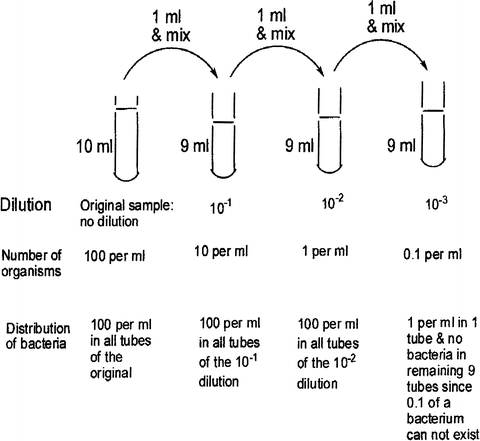

  

  The basis of the MPN technique (Drawn by the author: see text)

  The MPN is thus counting by the method of “dilution to extinction” made more accurate by the use of several tubes. For precise estimates, a very large number of tubes should be inoculated at each dilution. The confidence intervals can be narrowed by inoculating more tubes at each dilution or by using a smaller dilution ratio; a twofold dilution gives a greater precision than four-, five-, or tenfold dilution. If the microbial population size is not known, it is best to use a tenfold dilution with at least five (but preferably more) tubes at each dilution. If some idea of the microbial population size is known, it is best to use a dilution of 2, even if fewer tubes are used. The MPN is read from tables. Details of this method are available in Standard Methods for the Determination of Water and Wastewater (Anonymous 2006). The number of organisms is recorded in terms of Most Probable Numbers (MPN). Figures obtained in MPN determinations are indices of numbers which, more probably than any others, would give the results shown by laboratory examination. It should be emphasized that they are not actual numbers which, when determined with the plate count, are usually much lower. MPN index and 95% confidence limits for various combinations of positive results, when five tubes are used for dilution (10, 1, and 0.1 ml), are given in Table 2.1.

  Table 2.1 Most probable number index and 95% confidence limits for five tube, three dilution series (From Standard Methods for the Examination of Water and Wastewater; Anonymous 2006. With permission)

• 3. The membrane filtration method

  The membrane filtration method consists in filtering a measured volume of the water sample through a membrane composed of cellulose esters and other materials. The bacteria present are retained on the surface of the membrane, and by incubating the membrane face upward on a suitable agar or liquid medium and temperature, colonies develop on the membrane which can then be counted. The volume of liquid chosen will depend on the expected bacterial density of the water and should be such that colonies developing on the membrane lie between 10 and 100.

  The advantages of the filtration method over the multiple-tube method are:

  • (a) Rapidity: It is possible to obtain direct counts of coliforms and E. coli in 18 h without the use of probability tables.

  • (b) Labor, media, and glassware are also saved.

  • (c) For testing water for fecal contamination, neither spore-bearing anaerobes nor mixtures of organisms which may give false presumptive reactions in MacConkey broth cause false positive results on membranes.

  • (d) A sample may be filtered on the spot or in a nearby laboratory with limited facilities instead of taking the liquid to the proper laboratory.

  Membranes have, however, the following disadvan­tages:

  • (a) They are unsuitable for waters of high turbidities, and in which the required organisms are low in number, since they can be blocked before enough organisms have been collected.

  • (b) For water testing, when non-coliforms predominate over coliforms, the former may overgrow the membrane and make counting of coliforms difficult.

  • (c) Similarly, in water testing, if non-gas producing lactose-fermenters predominate in the water, false results will be obtained.

  Membrane filters are used to count various microorganisms including bacteriophages. Standard Methods for the Determination of Water and Wastewater (Anonymous 2006) contains detailed information on this.

• 4. Dilution of water for viable counts (plate count or MPN)

  Depending on the load of bacteria expected in water, the water will need to be diluted before the determination of its bacterial content. Table 2.2 gives a possible range of dilutions of water and other consumable liquids, whose bacterial load may be determined by plate count or MPN determinations.

  Table 2.2 Possible dilution of water and some consumable fluids prior to viable counts determination (Modified from science.kennesaw.edu/∼bensign/aqmeth/bacteriawaterquality.doc)

5.2 Direct Methods

Direct methods involve direct visualization of the microorganisms using a microscope. The impulses may be transmitted to a set up which may be read off as graphs or other visual end points. As will be seen below, some direct methods are often combined with some of the cultural methods described above.

5.2.1 Light Microscopy

The most common method of enumerating total microbial cells is the direct counting of cell suspension in a counting chamber of known volume using a microscope. One such counting chamber is the Neubauer counting chamber which has grids to facilitate counting, usually done under a light microscope. More sophisticated direct counting methods do not use the human eye, but instead use sensors which according to the desired program may detect size or different kinds of organisms depending on which dye is used to identify which organism. The various approaches are discussed under the title microscopy, below.

• 1. Optical (light) microscopy

  The optical or light microscope uses visible light and a system of lenses to magnify images of small samples. The image can be detected directly by the eye, imaged on a photographic plate or captured digitally. In light microscopy, the wavelength of the light limits the resolution to around 0.2 μm. The shorter the wave length the greater the magnification of the image; hence, in order to gain higher resolution, the use of an electron beam with a far shorter wavelengths is used in electron microscopes. The light for the light microscope may be daylight. However, bright light similar to day light may be produced from mercury-vapor lamps or xenon-arc lamps. The Neubauer counter has wide applications including being used to count blood cells in animal and human pathology laboratories, apart from being used for bacterial counts.

• 2. Fluorescence microscopy

  In fluorescence microscopy, the object being stu­died is labeled with a fluorescent dye which gives the object one color, say red, but emits another color, say green. Some materials, for example, chlorophyll are innately fluorescent and are said to be auto-fluorescent. Most current fluorescence microscopes are operated in the epi-illumination mode (illumination and detection from one side of the sample) and hence the system is known as epifluorescence microscopy. The excitation, illumination, or oncoming light strikes the object on one (usually, the top) side and, as will be seen below, this further decreases the amount of excitation light entering the detector. The major components of a fluorescence microscope are (Fig. 2.3):

  Fig. 2.3

  

  Setup illustrating the principle of the epifluorescence microscope (From http://international.abbottmolecular.com/DiagramoftheFluorescenceMicroscope_8843.aspx. With permission)

  • (a) The light source (Xenon or Mercury arc-discharge lamp).

  • (b) The excitation (illumination) filter (which filters away light of other wavelengths leaving one of a specific wavelength or color).

  • (c) The dichroic mirror (or dichromatic beam splitter) which simultaneously reflects the illumination light to the object and allows the reflected fluorescent light (of a different wavelength or color from the illumination light) to pass through.

  • (d) The emission filter, which allows the much weaker fluorescence or reflected light to pass through, and filters away any illuminating light coming from the object (see Fig. 2.3). The filters and the dichroic mirror are selected in accordance with wavelengths of the illumination light and the reflected light peculiar to the fluorescent dye used.

  The epifluorescence microscope is widely used in biology. It is used to count microorganisms directly in fresh and marine water as well as in milk, ­clinical specimens, and in environmental materials. The bac­terial cells are captured on the surface of polycarbonate membrane filters, stained with a fluorescent dye such as acridine orange, and visualized using epifluorescence microscopy. The fluorochrome (fluorescent dye) which is currently popular is 4′, 6′ diamidino-2-phenyl indole (DAPI). When using fluorescence techniques, the sample is either stained and then filtered onto membrane filters, or the cells are stained on the filters. Fluorochrome – stained – cells counts give an estimate of total living heterotrophic bacterial population in aquatic environments. However, a large proportion of the total cells are sometimes in a metabolically inactive state.

  To get an estimate of metabolically active cells, a dehydrogenase stain assay can be employed. In this method, the active dehydrogenase enzyme reduces a synthetic water soluble, membrane permeable, straw colored tetrazolium salt converting it to a pink-red, water insoluble formozan. The proportion of cells that have accumulated pink formozan through enzymatic dehydrogenation of tetrazolium substrate represents metabolically active cells.

  It has also been used to characterize planktonic procaryotic populations. An image analysis system may be used to digitize the video image of autofluorescing or fluorochrome-stained cells in the microscope field. The digitized image can then be stored, edited, and analyzed for total count or individual cell size and shape parameters, and results can be printed as raw data, statistical summaries, or histograms (Sieracki et al. 1985).

• 3. The confocal laser scanning microscope

  The confocal laser scanning microscope (CLSM or LSCM) is now often used in biology (Prasad et al. 2007).

  It is called “confocal” (meaning the same focus) because the final image has the same focus as the point of focus in the object. When an object is imaged in the fluorescence microscope, the signal produced is from the full thickness of the specimen; on account of this, most of the image is out of focus to the observer. The pinhole aperture of the confocal microscope blocks out this out-of-focus light (dotted lights in Fig. 2.4) and thus light from above and below the point of focus in the object. Filtering away some of the light reduces the amount of light and thus also reduces the “visibility” of the focused part of the specimen. To make up for this, laser beams are used which produce extremely bright light at a fixed wavelength. Highly sensitive photomultiplier-detectors (PMTs) are used to pick up and multiply the reduced laser beam striking the image. The laser is focused on a fixed portion of the specimen (a square or rectangle) at a time using a motorized system of mirrors controlled by a ­computer. The computer also allows the system to scan sequential planes in the (opposite direction) Z-direction, and create overlays of all the in-focus Z section, and store them. The information can also be used to create three-dimensional images, or movie rotations of well-stained specimens (Schibler 2010).

  Fig. 2.4

  

  Diagram illustrating the principle of the confocal microscope (From http:/www.gonda.ucla.edu/bri_core/confocal.htm; Schibler 2010. With permission)

  The confocal microscope has several advantages over conventional optical microscopy including:

  • (a) Controllable depth of field through controllable three-dimensional (3D) reconstructions.

  • (b) The elimination of image degrading out-of-focus information, thus obtaining high resolution images.

  • (c) The ability to collect serial optical sections from thick specimens.

  The key feature of confocal microscopy is its ability to produce sharp images of thick specimens at various depths. Images are taken point-by-point and reconstructed with a computer, rather than projected through an eyepiece. First developed in 1953, it took another 30 years and the development of lasers for confocal microscopy to become a standard technique toward the end of the 1980s.

  In this system, a laser beam passes through a light source aperture and then is focused by an objective lens into a small focal volume within a fluorescent specimen. A mixture of emitted fluorescent light as well as reflected laser light from the illuminated spot is then recollected by the objective lens. A beam splitter separates the light mixture by allowing only the laser light to pass through and reflecting the fluorescent light into the detection apparatus. After passing a pinhole, the fluorescent light is detected by a photo-detection device (photomultiplier tube [PMT]) transforming the light signal into an electrical one which is recorded by a computer.

  The detector aperture obstructs the light that is not coming from the focal point, as shown by the dotted gray line in the image. The out-of-focus points are thus suppressed: most of their returning light is blocked by the pinhole. This results in sharper images compared to conventional fluorescence microscopy techniques and permits one to obtain images of various X-Y axis planes; for depth, the object is also scanned in the Z axis plane (Schibler 2010).

5.2.2 Electron Microscopy

Electron microscopes were developed due to the limitations of the light microscopes which are limited by the physics of light to 500× or 1000× magnification and a resolution of 0.2 μm. The desire in the early 1930s to study the fine details of the interior structures of organic cells such as the nucleus, mitochondria, etc., fueled this need. The transmission electron microscope (TEM) was the first type of electron microscope to be developed and is patterned exactly on the light transmission microscope except that a focused beam of electrons is used instead of light to “see” through the specimen. It was developed in Germany in 1931. The first of the other type of electron microscope, the scanning electron microscope (SEM) came out in 1942, but the commercial came out about 1965.

• 1. The transmission electron microscope (TEM)

  The ray of electrons is produced by a pin-shaped cathode heated up by electric current. The electrons are produced in a vacuum at high electric voltage. The higher the voltage, the shorter are the electron waves and the higher is the power of resolution. Modern powers of resolution range from 0.2 to 0.3 nm and magnification is around 300,000×. The electron microscope is like the light microscope; however, the “lens” is an electric coil generating an electromagnetic field. Specimens are thin, no more than 100 nm thick, and are “stained” with heavy metal salts to make them visible. The formed image is made visible on a fluorescent screen, or it is captured on photographic material. Photos taken with electron microscopes are always black and white. The degree of darkness corresponds to the electron density (i.e., differences in atom masses) of the candled preparation.

• 2. The scanning electron microscope (SEM)

  The path of the electron beam within the scanning electron microscope differs from that of the TEM and is based on television techniques. The method is suitable for the showing of preparations with electrically conductive surfaces. Biological objects have thus to be made conductive by coating with a thin layer of heavy metal, usually gold. The power of resolution is smaller than in transmission electron microscopes, but the depth of focus is much higher. Scanning electron microscopy is therefore also well suited for very low magnifications. The surface of the object is scanned with the electron beam point by point whereby secondary electrons are set free. The intensity of this secondary radiation is dependent on the angle of inclination of the object’s surface. The secondary electrons are collected by a detector placed at an angle at the side above the object. The image appears a little later on a viewing screen.

  A comparison of the light, transmission, and scanning microscopes is given in Table 2.3.

  Table 2.3 Comparison of the properties of the light, and transmission and scanning electron microscopes (From http://universe-review.ca/R11-13-microscopes.htm#top; Anonymous 2010)

5.2.3 Flow Cytometry

Flow cytometry comes from “cyto” for cell, and “meter” for measure in the word cytometer. The technology involves the use of a beam of laser light projected through a liquid stream that contains cells, or other particles in the size range of 0.2–150 μm dia­meter, which when struck by the focused light give out signals which are picked up by detectors. These signals are then converted for computer storage and data analysis, and can provide information about various cellular properties.

Cells flow one at a time through a region of interaction at the rate of over 1,000 cells per second. The biophysical properties detected are then correlated with the biological and biochemical properties of interest. The high throughput of cells allows for rare cells, which may have inherent or inducible differences, to be easily detected and identified from the remainder of the cell population.

In order to make the measurement of biological/biochemical properties of interest easier, the cells are usually stained with fluorescent dyes which bind specifically to cellular constituents. The dyes are excited by the laser beam and emit light at longer wavelengths. This emitted light is picked up by detectors, and the signals are converted to digital so that they may be stored for later display and analysis.

Flow cytometers also have the ability to selectively deposit cells from particular populations into tubes, or other collection vessels. These selected cells can then be used for further experiments, cultured, or stained with another dye/antibody and reanalyzed. The data can be displayed in a number of different formats, each having advantages and disadvantages. The common methods are histogram, or dotplots. A flow cytometer typically consists of the following:

• 1. Flow chamber

  Cells flow through the flow chamber one at a time very quickly, about 10,000 cells in 20 s or more often 500 cells per second.

• 2. Laser

  A small laser beam of very bright light hits the cells as they pass through the flow chamber. The way the light bounces off each cell gives information about the cell’s physical characteristics. Light bounced off at small angles is called forward scatter. Light bounced off in other directions is called side scatter.

• 3. Light detector

  The light detector processes the light signals and sends the information to the computer. Forward scatter tells you the size of the cell. Side scatter tells if the cell contains granules. Each type of cell in the immune system has a unique combination of forward and side scatter measurements, allowing you to count the number of each type of cell.

• 4. Filters

  The filters direct the light emitted by the fluorochromes (fluorescent dyes) to the color detectors.

• 5. Color detectors

  As the cells pass through the laser, the fluorochromes attached to the cells absorb light and then emit a specific color of light depending on the type of fluorochrome. The color detectors collect the different colors of light emitted by the fluorochromes and send them to a computer.

• 6. Computer

  The data from the light detector and the color detectors is sent to a computer and plotted on a histogram.

  Flow cytometers or flourescence activated cell sor­ters are instruments which analyze optical parameters of many individual cells in a short space of time. The sample flows through an orifice and across the path of a light source, usually a laser. Optical parameters like light scatter and fluorescence are measured on each cell by photodetectors. The signals received are processed by a computer. On the basis of predefined optical pro­perties, cells can be sorted and collected automatically. Some of the advantages of flow cytometry are:

  • (a) Rapid analysis of relatively large sample sizes, i.e., 10⁴–10⁶ cells per minute.

  • (b) Modifications of the technique allow detection of smaller and less abundant cells in natural water samples.

  A well-known application of the flow cytometer is the analysis of natural phytoplankton by auto-fluorescence. By this technique, cyanobacterial phototrophs are enumerated and separated from other phytoplankton based on phycoerythrin and chlorophyll fluorescence. The former fluoresces orange and the latter red.

5.3 Determination of Bacterial Mass

Bacterial mass may be determined by direct weight measurement, or indirectly by the measurement of metabolic activities of the organism. For the determination of growth yields, wet or dry weight estimations are commonly used. For evaluating metabolic and enzymatic activities, protein or nitrogen content of a bacterial suspension is determined.

5.3.1 Direct Methods

After centrifuging the cells, wet weight can be determined. Dry weight is determined after drying the cells to constant weight.

Nitrogen content and total carbon content can also be determined using well-known laboratory procedures such as the Association of Official Agricultural Chemists (AOAC) procedures.

5.3.2 Indirect Methods

Bacterial mass may be determined by measuring the turbidity of cell suspensions; production of carbon dioxide, oxygen uptake, or production of acid can also be related to microbial mass after a calibration of the values against known quantities. These methods are particularly useful with very low concentration of cells. Chlorophyll determination is also a useful method, especially for algae; synthesis of ATP has also been used as a function of rate of microbial activity or total biomass (Hodson et al. 1976).

References

Anonymous. (2006). Standard methods for the examination of water and wastewater. Washington, DC: American Public Health Association, American Water Works Association, and Water Environmental Association.
Anonymous (2010). Microscopes. http://universe-review.ca/R11-13-microscopes.htm#top. Accessed 11 Aug 2010.
Buck, J. D. (1977). The plate count in aquatic microbiology. In J. W. Costerton & R. R. Colwell (Eds.), Native aquatic bacteria: Enumeration, activity and ecology (pp. 19–25). Philadelphia: American Society for Testing and Materials.
Colwell, R. R. (1977). Enumeration of specific populations by the most-probable number (MPN) method. In J. W. Costerton & R. R. Colwell (Eds.), Native aquatic bacteria: Enumeration, activity and ecology (pp. 56–64). Philadelphia: American Society for Testing and Materials.
Hodson, R. E., Holm-Hansen, O., & Azam, F. (1976). Improved methodology for ATP determination in marine environments. Marine Biology, 34, 143–149.
Matthews, J. E. (1972). Glossary of aquatic ecological terms. Environmental Protection Agency. Distributed By: National Technical Information Service, U.S. Department of Commerce.
Prasad, V., Semwogerere, V., & Weeks, D. (2007). Confocal microscopy of colloids. Journal of Physics: Condensed Matter, 19, 113102.
Pugnaire, F., & Valladares, F. (Eds.). (2007). Functional plant ecology (2nd ed.). Baton Rogue: CRC Press.
Schibler, M. (2010). http://www.gonda.ucla.edu/bri_core/confocal.htm. Private communication.
Sieracki, M. E., Johnson, P. W., & Sieburth, J. M. (1985). Detection, enumeration, and sizing of planktonic bacteria by image-analyzed epifluorescence microscopy. Applied and Environmental Microbiology, 49, 799–810.
Sigee, D. (2005). Freshwater microbiology: Biodiversity and dynamic interactions of microorganisms in the aquatic environment. Chichester: Wiley.
Author information
Authors and Affiliations
Corresponding author
Rights and permissions
Copyright information
© 2011 Springer Science+Business Media B.V.
About this chapter
Cite this chapter
Okafor, N. (2011). Peculiarities of Water as an Environmental Habitat for Microorganisms. In: Environmental Microbiology of Aquatic and Waste Systems. Springer, Dordrecht. https://doi.org/10.1007/978-94-007-1460-1_2
Download citation
DOI: https://doi.org/10.1007/978-94-007-1460-1_2
Published:
Publisher Name: Springer, Dordrecht
Print ISBN: 978-94-007-1459-5
Online ISBN: 978-94-007-1460-1
eBook Packages: Earth and Environmental ScienceEarth and Environmental Science (R0)