Gyrotriangle Gyrocenters

Abstract

Interest in triangle centers has long history, the classical ones being the triangle centroid, orthocenter, incenter and circumcenter. A list of more than 3000 triangle centers is found in Kimberling (Clark Kimberling’s Encyclopedia of Triangle Centers—ETC, 2010). Hyperbolic triangles and their centers are of interest as well (Bottema in Can. J. Math. 10:502–506, 1958; Vermeer in Topol. Appl. 152(3):226–242, 2005; Demirel and Soyturk in Novi Sad J. Math. 38(2):33–39, 2008; Sonmez in Algebras Groups Geom. 26(1):75–79, 2009). The special relativistic approach of this book enables hyperbolic triangle centers to be determined along with relationships between them.

The hyperbolic triangle circumcenter, incenter and orthocenter are called, in gyrolanguage, the gyrotriangle circumgyrocenter, ingyrocenter and orthogyrocenter, respectively. These gyrocenters are determined in this chapter in terms of their gyrobarycentric coordinate representations with respect to the vertices of their reference gyrotriangles.

These keywords were added by machine and not by the authors. This process is experimental and the keywords may be updated as the learning algorithm improves.

1 Gyrotriangle Circumgyrocenter

Definition 7.1

The circumgyrocenter, O, of a gyrotriangle is the point in the gyrotriangle gyroplane equigyrodistant from the three gyrotriangle vertices.

Let O be the circumgyrocenter of gyrotriangle A ₁ A ₂ A ₃ in an Einstein gyrovector space $({\mathbb{R}}_{s}^{n},{\oplus },{\otimes })$, Fig. 7.1, and let (m ₁:m ₂:m ₃) be its gyrobarycentric coordinates with respect to the set S={A ₁,A ₂,A ₃}, (4.25), p. 90, so that

$$O=\frac{m_1\gamma_{_{A_1}}^{\phantom{1}}A_1+m_2\gamma_{_{A_2}}^{\phantom{1}}A_2+m_3\gamma_{_{A_3}}^{\phantom{1}}A_3}{m_1\gamma_{_{A_1}}^{\phantom{1}}+m_2\gamma_{_{A_2}}^{\phantom{1}}+m_3\gamma_{_{A_3}}^{\phantom{1}}}.$$

(7.1)

The gyrobarycentric coordinates m ₁,m ₂ and m ₃ are to be determined in (7.8) below, in terms of gamma factors of the gyrotriangle sides and, alternatively in (7.16), in terms of the gyrotriangle gyroangles.

Fig. 7.1

The circumgyrocenter O of gyrotriangle A ₁ A ₂ A ₃ in an Einstein gyrovector space $({\mathbb{R}}_{s}^{n},{\oplus },{\otimes })$, n=2, is shown along with its standard notation. Here ‖⊖ A ₁⊕O‖ = ‖⊖ A ₂⊕O‖ = ‖⊖ A ₃⊕O‖, where O is the gyrotriangle circumgyrocenter, given by its gyrobarycentric coordinate representation (7.18), with respect to the set S={A ₁,A ₂,A ₃}

Following the gyrocovariance of gyrobarycentric coordinate representations, Theorem 4.6, we have from Identity (4.29b), p. 91, with X=⊖ A ₁, using the standard gyrotriangle index notation, shown in Fig. 7.1, in Fig. 6.1, p. 128, and in (6.1), p. 127,

(7.2)

where by (4.15), p. 88, the circumgyrocenter constant m ₀>0 with respect to the set of the gyrotriangle vertices is given by the equation

$$m_0^2=m_1^2+m_2^2+m_3^2+2(m_1m_2\gamma_{12}^{\phantom{O}}+m_1m_3\gamma_{13}^{\phantom{O}}+m_2m_3\gamma_{23}^{\phantom{O}}).$$

(7.3)

Hence, similarly, by the gyrocovariance of gyrobarycentric coordinate representations, Identity (4.29b), p. 91, of Theorem 4.6 with X=⊖ A ₁, with X=⊖ A ₂, and with X=⊖ A ₃, we have, respectively,

(7.4)

The condition that the circumgyrocenter O is equigyrodistant from its gyrotriangle vertices A ₁,A ₂, and A ₃ implies

$$\gamma_{_{{\ominus }A_1{\oplus }O}}^{\phantom{1}}=\gamma_{_{{\ominus }A_2{\oplus }O}}^{\phantom{1}}=\gamma_{_{{\ominus }A_3{\oplus }O}}^{\phantom{1}}.$$

(7.5)

Equations (7.4) and (7.5), along with the normalization condition m ₁+m ₂+m ₃=1, yield the following system of three equations for the three unknowns m ₁,m ₂, and m ₃,

(7.6)

which can be written as the matrix equation,

$$\begin{pmatrix}1&1&1\\[4pt]1-\gamma_{13}^{\phantom{1}}&\gamma_{12}^{\phantom{1}}-\gamma _{23}^{\phantom{1}}&\gamma_{13}^{\phantom{1}}-1\\[4pt]\gamma_{12}^{\phantom{1}}-\gamma_{13}^{\phantom{1}}&1-\gamma _{23}^{\phantom{1}}&\gamma_{23}^{\phantom{1}}-1\end{pmatrix}\begin{pmatrix}m_1\\[4pt]m_2\\[4pt]m_3\end{pmatrix}=\begin{pmatrix}1\\[4pt]0\\[4pt]0\end{pmatrix}.$$

(7.7)

Solving (7.7) for the unknowns m ₁,m ₂, and m ₃, we have

(7.8)

where D is the determinant of the 3×3 matrix in (7.7),

(7.9)

Hence, the circumgyrocenter O of gyrotriangle A ₁ A ₂ A ₃ is given by (7.1) where gyrobarycentric coordinates m ₁,m ₂, and m ₃ are given by (7.8). Since in gyrobarycentric coordinates only ratios of coordinates are relevant, the gyrobarycentric coordinates, m ₁,m ₂, and m ₃ in (7.8) can be simplified by removing their common factor 1/D.

Gyrobarycentric coordinates, m ₁,m ₂, and m ₃, of the circumgyrocenter O of gyrotriangle A ₁ A ₂ A ₃ are thus given by the equations

(7.10)

Hence, by (7.3) along with the gyrobarycentric coordinates in (7.10), we have

(7.11)

According to Corollary 4.9, p. 93, the gyrotriangle A ₁ A ₂ A ₃ in Fig. 7.1 possesses a circumgyrocenter if and only if $m_{0}^{2}>0$.

The second factor of $m_{0}^{2}$ in (7.11) is positive for any gyrotriangle A ₁ A ₂ A ₃ in an Einstein gyrovector space, by Inequality (6.23), p. 135. Hence, as we see from (7.11), $m_{0}^{2}>0$ if and only if the points A ₁, A ₂, and A ₃ obey the circumgyrocircle condition

$$(\gamma_{12}^{\phantom{O}}+\gamma_{13}^{\phantom{O}}+\gamma _{23}^{\phantom{O}}-1)^2>2\bigl(\gamma_{12}^2+\gamma _{13}^2+\gamma_{23}^2-1\bigr).$$

(7.12)

Gamma factors of gyrotriangle side gyrolengths are related to its gyroangles by the equations, (6.33), p. 137,

(7.13)

Substituting these from (7.13) into (7.10), we obtain

(7.14)

where the common factor F in (7.14) is given by the equation

$$F=2^3\frac{\cos^2(\frac{\alpha_1+\alpha_2+\alpha_3}{2})\cos(\frac{-\alpha_1+\alpha_2+\alpha_3}{2})\cos(\frac{\alpha_1-\alpha_2+\alpha_3}{2})\cos(\frac{\alpha_1+\alpha_2-\alpha_3}{2})}{\sin\alpha_1\sin\alpha_2\sin\alpha_3}.$$

(7.15)

Since in gyrobarycentric coordinates only ratios of coordinates are relevant, the gyrobarycentric coordinates, $m_{1}^{\prime},m_{2}^{\prime}$, and $m_{3}^{\prime}$ in (7.14) can be simplified by removing their common factor F. Hence, gyrobarycentric coordinates, $m_{1}^{\prime\prime},m_{2}^{\prime\prime}$, and $m_{3}^{\prime\prime }$, of the circumgyrocenter O of gyrotriangle A ₁ A ₂ A ₃, expressed in terms of the gyrotriangle gyroangles are given by the equations

(7.16)

By Corollary 4.10, p. 94, the circumgyrocenter O, (7.1), lies on the interior of its gyrotriangle A ₁ A ₂ A ₃ if and only if all its gyrobarycentric coordinates are positive. Hence, we see from the gyrobarycentric coordinates (7.16) of O that the circumgyrocenter O lies on the interior of its gyrotriangle A ₁ A ₂ A ₃ if and only if the largest gyroangle of the gyrotriangle has measure less than the sum of the measures of the other two gyroangles. This result is known in hyperbolic geometry; see, for instance, [28, p. 132], where the result is proved synthetically.

Expressing Inequality (7.12) gyrotrigonometrically, by means of (7.13), it can be shown that $m_{0}^{2}>0$ if and only if

(7.17)

Formalizing the main result of this section, we have the following theorem:

Theorem 7.2

(The Circumgyrocenter) Let S={A ₁,A ₂,A ₃} be a pointwise independent set of three points in an Einstein gyrovector space $({\mathbb{R}}_{s}^{n},{\oplus },{\otimes })$. The circumgyrocenter O∈ℝⁿ, Fig. 7.1, of gyrotriangle A ₁ A ₂ A ₃ has the gyrobarycentric coordinate representation

$$O=\frac{m_1\gamma_{_{A_1}}^{\phantom{1}}A_1+m_2\gamma_{_{A_2}}^{\phantom{1}}A_2+m_3\gamma_{_{A_3}}^{\phantom{1}}A_3}{m_1\gamma_{_{A_1}}^{\phantom{1}}+m_2\gamma_{_{A_2}}^{\phantom{1}}+m_3\gamma_{_{A_3}}^{\phantom{1}}}$$

(7.18)

with respect to the set S={A ₁,A ₂,A ₃}, with gyrobarycentric coordinates (m ₁:m ₂:m ₃) given by

(7.19)

or, equivalently, by the gyrotrigonometric gyrobarycentric coordinates

(7.20)

The circumgyrocenter constant m ₀ with respect to the set S={A ₁,A ₂,A ₃} is given by the equation

(7.21)

The circumgyrocenter lies in the ball, $O\in {\mathbb{R}}_{s}^{n}$, if and only if $m_{0}^{2}>0$.

2 Triangle Circumcenter

In this section the gyrotriangle circumgyrocenter in Fig. 7.1 will be translated into its Euclidean counterpart in Fig. 7.2.

Fig. 7.2

The circumcenter O of triangle A ₁ A ₂ A ₃ in a Euclidean vector space ℝⁿ, n=2, is shown along with its standard notation. Here ‖−A ₁+O‖ = ‖−A ₂+O‖ = ‖−A ₃+O‖, where O is the triangle circumcenter, given by its barycentric coordinate representation (7.23) with respect to the set S={A ₁,A ₂,A ₃}

Interestingly, the gyrobarycentric coordinate representation (7.18) with gyrotrigonometric gyrobarycentric coordinates (m ₁:m ₂:m ₃) given by (7.20) remains invariant in form under the Euclidean limit s→∞, so that it is valid in Euclidean geometry as well. However, for application in Euclidean geometry the representation (7.18) can be simplified owing to the fact that triangle angle sum in π.

Indeed, under the condition

$$\alpha_1+\alpha_2+\alpha_3=\pi,\quad \mbox{(Euclidean~Geometry)}$$

(7.22a)

we have the trigonometric identities

(7.22b)

that allow m _k , k=1,2,3, in (7.20) to be simplified.

Thus, ignoring a common factor 2, the trigonometric barycentric coordinates (7.20) of the triangle circumcenter O give rise to the following simpler trigonometric barycentric coordinates:

(7.22c)

Hence, finally, a trigonometric barycentric coordinate representation of the circumcenter O of triangle A ₁ A ₂ A ₃ in Fig. 7.2 with respect to the set S={A ₁,A ₂,A ₃} is given by (7.23) of the following corollary of Theorem 7.2, which recovers a well-known result in Euclidean geometry [29]:

Corollary 7.3

Let α _k , k=1,2,3, and O be the angles and circumcenter of a triangle A ₁ A ₂ A ₃ in a Euclidean space ℝⁿ. Then,

$$O=\frac{\sin2\alpha_1A_1+\sin2\alpha_2A_2+\sin2\alpha_3A_3}{\sin2\alpha_1+\sin2\alpha_2+\sin2\alpha_3}\quad (\mathrm{Euclidean~Geometry})$$

(7.23)

Theorem 7.2 and its Corollary 7.3 form an elegant example that illustrates the result that

• (i) Gyrotrigonometric gyrobarycentric coordinates of a point in an Einstein gyrovector space ${\mathbb{R}}_{s}^{n}$ survive unimpaired in Euclidean geometry, where they form.

• (ii) Trigonometric barycentric coordinates of a point in a corresponding Euclidean vector space ℝⁿ.

  The converse is, however, not valid:

• (iii) Trigonometric barycentric coordinates of a point in a Euclidean vector space ℝⁿ may embody the Euclidean condition the triangle angle sum in π, so that they need not survive in hyperbolic geometry.

3 Gyrocircle

The gyrocircle C(r,O) with gyroradius r, 0<r<s, and gyrocenter $O\in{\mathbb{R}}_{s}^{2}$ in an Einstein gyrovector plane $({\mathbb{R}}_{s}^{2},{\oplus },{\otimes })$ is the set of all points $P\in{\mathbb{R}}_{s}^{2}$ such that ‖⊖ P⊕O‖=r; see Fig. 7.3. It is given by the equation

$$C(r,O,\theta)=O~{\oplus }\begin{pmatrix}r\cos\theta\\r\sin\theta \end{pmatrix}$$

(7.24)

for 0≤θ<2π. Indeed, by the left cancellation law we have

$$\bigl\|{\ominus }O{\oplus }C(r,O,\theta)\bigr\|=\left\|\begin{pmatrix}r\cos\theta\\r\sin\theta \end{pmatrix}\right\|=r,$$

(7.25)

where ‖⋅‖ is the norm that the Einstein gyrovector plane ${\mathbb{R}}_{s}^{2}$ inherits from its Euclidean plane ℝ².

Fig. 7.3

A sequence of gyrocircles with gyroradius $\frac{1}{4}$ in an Einstein gyrovector plane ${\mathbb{R}}_{s=1}^{2}$ with gyrocenters approaching the boundary of the open unit disc ${\mathbb{R}}_{s=1}^{2}$ is shown. The center of the disc is conformal. Hence, the gyrocircle with gyrocenter at the center of the disc coincides with a Euclidean circle. The Euclidean circle is increasingly flattened as its gyrocenter approaches the boundary of the disc

A sequence of gyrocircles of gyroradius $\frac{1}{4}$ in an Einstein gyrovector plane ${\mathbb{R}}_{s=1}^{2}$ with gyrocenters approaching the boundary of the open unit disc ${\mathbb{R}}_{s=1}^{2}$ is shown in Fig. 7.3. The center of the disc in Fig. 7.3 is conformal, as explained in Sect. 2.6, p. 53. Accordingly, a gyrocircle with gyrocenter at the center of the disc is identical to a Euclidean circle. This Euclidean circle is increasingly flattened in the Euclidean sense when the gyrocircle gyrocenter approaches the boundary of the disc.

The circumgyrocircle of gyrotriangle A ₁ A ₂ A ₃ in Fig. 7.1, with circumgyrocenter at the point O, is shown in Fig. 7.4.

Fig. 7.4

The circumgyrocircle of gyrotriangle A ₁ A ₂ A ₃ in an Einstein gyrovector space $({\mathbb{R}}_{s}^{n},{\oplus },{\otimes })$ is shown for n=2. Its gyrocenter, O, is the gyrotriangle circumgyrocenter, given by its gyrobarycentric representation (7.18), p. ??, and its gyroradius r is the gyrotriangle circumgyroradius, given by each of the equations r=‖⊖ A _k ⊕O‖, k=1,2,3. The gyrocircle is a flattened Euclidean circle, as shown in Fig. 7.3

4 Gyrotriangle Circumgyroradius

In this section, we face the task of calculating the gyrotriangle circumgyroradius. The circumgyroradius R of gyrotriangle A ₁ A ₂ A ₃ in Figs. 7.1 and 7.4 is given by

$$R=\|{\ominus }A_1{\oplus }O\|=\|{\ominus }A_2{\oplus }O\|=\|{\ominus }A_3{\oplus }O\|$$

(7.26)

satisfying, by (7.2),

$$\gamma_{_{R}}^{\phantom{1}}=\gamma_{_{{\ominus }A_1{\oplus }O}}^{\phantom{1}}=\frac{m_1+m_2\gamma_{12}^{\phantom{O}}+m_3\gamma_{13}^{\phantom{O}}}{m_0},$$

(7.27)

where m ₁,m ₂ and m ₃ are given by (7.19), and where m ₀ is given by (7.21).

Hence, following (7.27), (7.19) and (7.21), we have

$$\gamma_R^2=\frac{2\gamma_{12}^{\phantom{O}}\gamma_{13}^{\phantom{O}}\gamma _{23}^{\phantom{O}}-(\gamma_{12}^2+\gamma_{13}^2+\gamma_{23}^2-1)}{(\gamma_{12}^{\phantom{O}}+\gamma_{13}^{\phantom{O}}+\gamma _{23}^{\phantom{O}}-1)^2-2(\gamma_{12}^2+\gamma _{13}^2+\gamma_{23}^2-1)}$$

(7.28)

so that, by (1.9), p. 5,

$$R^2=s^2\frac{\gamma_R^2-1}{\gamma_R^2}=2s^2\frac{(\gamma_{12}^{\phantom{O}}-1)(\gamma_{13}^{\phantom{O}}-1)(\gamma _{23}^{\phantom{O}}-1)}{1+2\gamma_{12}^{\phantom{O}}\gamma_{13}^{\phantom{O}}\gamma _{23}^{\phantom{O}}-\gamma_{12}^2-\gamma_{13}^2-\gamma_{23}^2}.$$

(7.29)

Hence, finally, the circumgyroradius R of gyrotriangle A ₁ A ₂ A ₃ in Figs. 7.1 and 7.4 is given by

$$R=\sqrt{2}s\sqrt{\frac{(\gamma_{12}^{\phantom{O}}-1)(\gamma_{13}^{\phantom{O}}-1)(\gamma _{23}^{\phantom{O}}-1)}{1+2\gamma_{12}^{\phantom{O}}\gamma_{13}^{\phantom{O}}\gamma _{23}^{\phantom{O}}-\gamma_{12}^2-\gamma_{13}^2-\gamma_{23}^2}},$$

(7.30)

implying

$$\sqrt{\frac{(\gamma_{12}^{\phantom{O}}+1)(\gamma_{13}^{\phantom{O}}+1)(\gamma _{23}^{\phantom{O}}+1)}{2}}R=s\sqrt{\frac{(\gamma_{12}^2-1)(\gamma_{13}^2-1)(\gamma_{23}^2-1)}{1+2\gamma_{12}^{\phantom{O}}\gamma_{13}^{\phantom{O}}\gamma _{23}^{\phantom{O}}-\gamma_{12}^2-\gamma_{13}^2-\gamma_{23}^2}}.$$

(7.31)

Identity (7.31) captures a remarkable analogy between the law of gyrosines and the law of sines. Indeed, following (7.31), the law of gyrosines (6.44), p. 140, for gyrotriangle A ₁ A ₂ A ₃ in Fig. 7.4 is linked to the circumgyroradius R of the gyrotriangle by the equation

$$\frac{\gamma_{23}^{\phantom{O}}a_{23}}{\sin\alpha_1}=\frac{\gamma_{13}^{\phantom{O}}a_{13}}{\sin\alpha_2}=\frac{\gamma_{12}^{\phantom{O}}a_{12}}{\sin\alpha_3}=\sqrt{\frac{(\gamma_{12}^{\phantom{O}}+1)(\gamma_{13}^{\phantom{O}}+1)(\gamma _{23}^{\phantom{O}}+1)}{2}}R$$

(7.32)

called the extended law of gyrosines.

In the Euclidean limit of large s, s→∞, gamma factors tend to 1 and, accordingly, the extended law of gyrosines (7.32) tends to the following identity,

$$\frac{a_{23}}{\sin\alpha_1}=\frac{a_{13}}{\sin\alpha_2}=\frac{a_{12}}{\sin\alpha_3}=2R\quad \mbox{(Euclidean~Geometry)}$$

(7.33)

which is the well-known extended law of sines; see, for instance, [35, p. 87].

Identity (7.32) forms the extended law of gyrosines of a gyrotriangle A ₁ A ₂ A ₃ with side-gyrolengths a ₂₃,a ₁₃,a ₁₂, with gyroangles α ₁,α ₂,α ₃, and with circumgyroradius R. In full analogy, with (7.32), Identity (7.33) forms the Euclidean extended law of sines of a triangle A ₁ A ₂ A ₃ with side-lengths a ₂₃,a ₁₃,a ₁₂, with angles α ₁,α ₂,α ₃, and with circumradius R.

Interestingly, the gyrotriangle circumgyroradius R has an elegant representation in terms of its gyrotriangle gyroangles. Indeed, expressing the gamma factors in (7.29) in terms of the gyrotriangle gyroangles α _k , k=1,2,3, by means of (6.33), p. 137, (7.29) takes the gyrotrigonometric form

$$\frac{R^2}{s^2}=\frac{\cos\frac{\alpha_1+\alpha_2+\alpha_3}{2}}{\cos\frac{\alpha_1-\alpha_2-\alpha_3}{2}\cos\frac{-\alpha_1+\alpha_2-\alpha_3}{2}\cos\frac{-\alpha_1-\alpha_2+\alpha_3}{2}}$$

(7.34)

in any Einstein gyrovector space $({\mathbb{R}}_{s}^{n},{\oplus },{\otimes })$. In the Euclidean limit, s→∞, each side of (7.34) tends to 0. Indeed, in that limit, the gyroangle gyrotriangle sum α ₁+α ₂+α ₃ tends to π so that $\cos\frac{\alpha_{1}+\alpha_{2}+\alpha_{3}}{2}$ tends to 0.

An important relation that results from (7.34) is formalized in the following theorem:

Theorem 7.4

Let α _k , k=1,2,3, and R be the gyroangles and circumgyroradius of a gyrotriangle A ₁ A ₂ A ₃ in an Einstein gyrovector space $({\mathbb {R}}_{s}^{n}{\oplus },{\otimes })$. Then

(7.35)

Interestingly, the Euclidean limit, s→∞, of the left-hand side of Identity (7.35) of Theorem 7.4 is an indeterminate limit of type ∞⋅0, noting that in that limit α ₁+α ₂+α ₃ tends to π so that $\cos\frac{\alpha_{1}+\alpha_{2}+\alpha_{3}}{2}$ tends to 0. In contrast, the right-hand side of the identity remains invariant in form in that limit. An elegant application of Theorem 7.4 is encountered in (8.24), p. 230, where a hyperbolic geometric identity is obtained, which remains invariant in form in its transition to Euclidean geometry.

5 The Gyrocircle Through Three Points

In the following theorem, we use the standard gyrotriangle index notation, shown in Fig. 6.1, p. 128, and in (6.1), p. 127.

Theorem 7.5

(The Gyrocircle Through Three Points) Let A ₁, A ₂ and A ₃ be any three distinct points in an Einstein gyrovector space $({\mathbb{R}}_{s}^{n},{\oplus },{\otimes })$, see Figs. 7.5 – 7.6. There exists a unique gyrocircle that passes through these points if and only if these points obey the circumgyrocircle condition, (7.12),

$$(\gamma_{12}^{\phantom{O}}+\gamma_{13}^{\phantom{O}}+\gamma _{23}^{\phantom{O}}-1)^2>2\bigl(\gamma_{12}^2+\gamma _{13}^2+\gamma_{23}^2-1\bigr).$$

(7.36)

When a gyrocircle exists, it is the unique gyrocircle with gyrocenter O given by, (7.18),

$$O=\frac{m_1\gamma_{_{A_1}}^{\phantom{1}}A_1+m_2\gamma_{_{A_2}}^{\phantom{1}}A_2+m_3\gamma_{_{A_3}}^{\phantom{1}}A_3}{m_1\gamma_{_{A_1}}^{\phantom{1}}+m_2\gamma_{_{A_2}}^{\phantom{1}}+m_3\gamma_{_{A_3}}^{\phantom{1}}},$$

(7.37)

where

(7.38)

and with gyroradius R given as in (7.30), i.e.,

$$R=\sqrt{2}s\sqrt{\frac{(\gamma_{12}^{\phantom{O}}-1)(\gamma_{13}^{\phantom{O}}-1)(\gamma _{23}^{\phantom{O}}-1)}{1+2\gamma_{12}^{\phantom{O}}\gamma_{13}^{\phantom{O}}\gamma _{23}^{\phantom{O}}-\gamma_{12}^2-\gamma_{13}^2-\gamma_{23}^2}}.$$

(7.39)

Fig. 7.5

Here A ₁, A ₂ and A ₃ are arbitrarily selected three points of an Einstein gyrovector space $({\mathbb{R}}_{s}^{n},{\oplus },{\otimes })$ that satisfy the circumgyrocircle condition (7.36). Accordingly, there exists a unique gyrocircle that passes through these points

Fig. 7.6

Here A ₁, A ₂ and A ₃ are arbitrarily selected three points of an Einstein gyrovector space $({\mathbb{R}}_{s}^{n},{\oplus },{\otimes })$ that do not satisfy the circumgyrocircle condition (7.36). Accordingly, there exists no gyrocircle that passes through these points

Proof

The gyrocircle in the theorem, if exists, is the circumgyrocircle of gyrotriangle A ₁ A ₂ A ₃. The gyrocenter O of the gyrocircle is, therefore, given by (7.37)–(7.38), as we see from Theorem 7.2, p. ??; and the gyroradius, R, of the gyrocircle is given by (7.30), p. ??.

Finally, the circumgyrocircle of gyrotriangle A ₁ A ₂ A ₃ exists if and only if the points A ₁, A ₂ and A ₃ satisfy the circumgyrocircle condition (7.36), as explained in the paragraph of Inequality (7.12), p. ??. □

Example 7.6

If the three points A ₁, A ₂ and A ₃ in Theorem 7.5 are not distinct, a gyrocircle through these points is not unique. Indeed, in this case we have

$$(\gamma_{12}^{\phantom{O}}+\gamma_{13}^{\phantom{O}}+\gamma _{23}^{\phantom{O}}-1)^2=2\bigl(\gamma_{12}^2+\gamma _{13}^2+\gamma_{23}^2-1\bigr),$$

(7.40)

as one can readily check, thus violating the circumgyrocircle condition (7.36).

Example 7.7

If the three points A ₁, A ₂ and A ₃ in Theorem 7.5 are distinct and gyrocollinear, there is no gyrocircle through these points. Hence, in this case the circumgyrocircle condition (7.36) must be violated. Hence, these points must satisfy the inequality

$$(\gamma_{12}^{\phantom{O}}+\gamma_{13}^{\phantom{O}}+\gamma _{23}^{\phantom{O}}-1)^2\le 2\bigl(\gamma_{12}^2+\gamma _{13}^2+\gamma_{23}^2-1\bigr).$$

(7.41)

Example 7.8

Let the three points A ₁, A ₂ and A ₃ in Theorem 7.5 be the vertices of an equilateral gyrotriangle with side gyrolengths a. Then, $\gamma_{12}^{\phantom{O}}=\gamma _{13}^{\phantom{O}}=\gamma_{23}^{\phantom{O}}=\gamma _{a}^{\phantom{.}}$, so that the circumgyrocircle condition (7.36) reduces to

$$\gamma_a^{\phantom{O}}>1$$

(7.42)

which is satisfied by any side gyrolength a, 0<a<s.

Hence, by Theorem 7.5, any equilateral gyrotriangle in an Einstein gyrovector space possesses a circumgyrocircle.

6 The Inscribed Gyroangle Theorem

In Fig. 7.7, we use a notation that includes the standard gyrotriangle index notation, shown in Fig. 6.1, p. 128, and in (6.1), p. 127. Fig. 7.7 presents a gyrotriangle A ₁ A ₂ A ₃ and its circumgyrocircle with gyrocenter O at the gyrotriangle ingyrocenter, given by (7.18), p. ??, and with gyroradius R, given by the gyrotriangle circumgyroradius (7.30), p. ??. The gamma factor γ _R of R is given by (7.28), p. ??.

Fig. 7.7

The Inscribed Gyroangle Theorem. Illustrating the theorem, θ=∠ A ₁ A ₃ A ₂ is a gyroangle inscribed in a gyrocircle of gyroradius R (the circumgyroradius of gyrotriangle A ₁ A ₂ A ₃) centered at O in an Einstein gyrovector plane $({\mathbb{R}}_{s}^{2},{\oplus },{\otimes })$, and φ=∠ A ₁ OM ₁₂=∠ A ₂ OM ₁₂, where M ₁₂ is the gyromidpoint of the gyrosegment A ₁ A ₂. Accordingly, 2φ=∠ A ₁ OA ₂ is a gyrocentral gyroangle, and both θ and 2φ subtend on the same gyroarc on the gyrocircle. The elegant relationship between θ and φ, (7.43), is shown. In the Euclidean limit of large s, s→∞, gamma factors tend to 1 and, hence, the relationship between θ and φ in Euclidean geometry becomes sin θ=sin φ or, equivalently, θ=φ

Theorem 7.9

(The Inscribed Gyroangle Theorem) Let θ be a gyroangle inscribed in a gyrocircle of gyroradius R, and let 2φ be a gyrocentral gyroangle such that both θ and 2φ subtend on the same gyroarc on the gyrocircle, as shown in Fig. 7.7. Then, in the notation of Fig. 7.7 and (6.1), p. 127,

$$\sin\theta=\frac{2\gamma_R}{\sqrt{(\gamma_{13}^{\phantom{O}}+1)(\gamma_{23}^{\phantom{O}}+1)}}\sin\phi.$$

(7.43)

Proof

Under the conditions of the theorem, as described in Fig. 7.7, let M ₁₂ be the gyromidpoint of gyrosegment A ₁ A ₂, implying

$$\phi:=\angle A_1OM_{12}=\angle A_2OM_{12}=\frac{1}{2}\angle A_1OA_2$$

(7.44)

so that 2φ is the gyrocentral gyroangle ∠ A ₁ OA ₂ shown in Fig. 7.7.

Furthermore, let

$$\mathbf{a}_{12}={\ominus }A_1{\oplus }A_2$$

(7.45)

so that, by (4.67), p. 100,

$${\ominus }A_1{\oplus }M_{12}=\frac{1}{2}{\otimes }\mathbf{a}_{12},$$

(7.46)

and hence, by (4.69), p. 100,

$$\gamma_{\frac{1}{2}{\otimes }\mathbf{a}_{12}}^{\phantom{O}}\biggl(\frac {1}{2}{\otimes }\mathbf{a}_{12}\biggr)=\frac{\gamma_{12}^{\phantom{O}}\mathbf{a}_{12}}{\sqrt{2}\sqrt{1+\gamma_{12}^{\phantom{O}}}}.$$

(7.47)

Taking magnitudes of both sides of (7.47), we have

$$\gamma_{\frac{1}{2}{\otimes }a_{12}}^{\phantom{O}}\biggl(\frac{1}{2}{\otimes }a_{12}\biggr)=\frac{\gamma_{12}^{\phantom{O}}a_{12}}{\sqrt{2}\sqrt{1+\gamma_{12}^{\phantom{O}}}}.$$

(7.48)

Applying the extended law of gyrosines (7.32), p. ??, to gyrotriangle A ₁ A ₂ A ₃ and its circumgyrocircle in Fig. 7.7, we have

$$\frac{\gamma_{12}^{\phantom{O}}a_{12}}{\sin\theta}=\sqrt{\frac{(\gamma_{12}^{\phantom{O}}+1)(\gamma_{13}^{\phantom{O}}+1)(\gamma _{23}^{\phantom{O}}+1)}{2}}R,$$

(7.49)

implying

$$\sin\theta=\frac{\sqrt{2}\gamma_{12}^{\phantom{O}}a_{12}}{\sqrt{(1+\gamma_{12}^{\phantom{O}})(1+\gamma_{13}^{\phantom{O}})(1+\gamma_{23}^{\phantom{O}})}R}.$$

(7.50)

Applying the elementary gyrosine definition in gyrotrigonometry, (6.65), p. 146, illustrated in Fig. 6.5, p. 147, to the right gyroangled gyrotriangle A ₁ M ₁₂ O in Fig. 7.7, we obtain the first equation in (7.51),

$$\sin\phi=\frac{\gamma_{\frac{1}{2}{\otimes }a_{12}}^{\phantom{O}}(\frac{1}{2}{\otimes }a_{12})}{\gamma_RR}=\frac{\gamma_{12}^{\phantom{O}}a_{12}}{\sqrt{2}\sqrt{1+\gamma_{12}^{\phantom{O}}}~\gamma_RR}.$$

(7.51)

The second equation in (7.51) follows from (7.48).

Finally, the desired identity (7.43) follows immediately from (7.50) and (7.51). □

7 Gyrotriangle Gyroangle Bisector Foot

A gyrotriangle A ₁ A ₂ A ₃ and its gyroangle bisectors in an Einstein gyrovector space $({\mathbb{R}}_{s}^{n},{\oplus },{\otimes })$ are presented in Fig. 7.8, along with the gyrotriangle standard notation in Fig. 6.1, p. 128, and in (6.1), p. 127.

Fig. 7.8

The gyrotriangle gyroangle bisectors are concurrent. The point of concurrency, I, is called the ingyrocenter of the gyrotriangle. Let A ₁ A ₂ A ₃ be a gyrotriangle in an Einstein gyrovector space $({\mathbb{R}}_{s}^{n},{\oplus },{\otimes })$. The gyroline A _k P _k is the gyroangle bisector from vertex A _k to the intersection point P _k with the opposite side, k=1,2,3. The point P _k is the foot of the gyroangle bisector A _k P _k

Let P ₃ be a point on side A _! A ₂ of gyrotriangle A ₁ A ₂ A ₃ in an Einstein gyrovector space $({\mathbb{R}}_{s}^{n}{\oplus },{\otimes })$ such that A ₃ P ₃ is the gyroangle bisector of gyroangle ∠ A ₁ A ₃ A ₂, as shown in Fig. 7.8 for n=2. Then, the point P ₃ is the foot of the gyroangle bisector A ₃ P ₃ in gyrotriangle A ₁ A ₂ A ₃.

Let P ₃ be given in terms of its gyrobarycentric coordinates (m ₁:m ₂) with respect to the set S={A ₁,A ₂} by the equation

$$P_3=\frac{m_1\gamma_{_{A_1}}A_1+m_2\gamma_{_{A_2}}A_2}{m_1\gamma_{_{A_1}}+m_2\gamma_{_{A_2}}}.$$

(7.52)

The gyrobarycentric coordinates m ₁ and m ₂ of P ₃, Fig. 7.8, in (7.52) are to be determined in (7.68) below in terms of gyroangles α ₁ and α ₂ of the gyrotriangle A ₁ A ₂ A ₃ and in (7.69) in terms of the side gyrolengths of the gyrotriangle.

Following the gyrocovariance of gyrobarycentric coordinate representations, Theorem 4.6, p. 90, the gyrobarycentric coordinate representation of the point P ₃ in (7.52) gives rise to the identities in (7.53)–(7.55) below:

$${\ominus }X{\oplus }P_3=\frac{m_1\gamma_{_{{\ominus }X{\oplus }A_1}}^{\phantom{O}}({\ominus }X{\oplus }A_1)+m_2\gamma_{_{{\ominus }X{\oplus }A_2}}^{\phantom{O}}({\ominus }X{\oplus }A_2)}{m_1\gamma_{_{{\ominus }X{\oplus }A_1}}^{\phantom{O}}+m_2\gamma_{_{{\ominus }X{\oplus }A_2}}^{\phantom{O}}}$$

(7.53)

and

(7.54)

for any $X\in{\mathbb{R}}_{s}^{n}$, where, in the notation of Fig. 7.8 for the gamma factor $\gamma_{12}^{\phantom{O}}$, the constant m ₀>0 in (4.28d), p. 91, specializes to

$$m_0^2=(m_1+m_2)^2+2m_1m_2(\gamma_{12}^{\phantom{O}}-1)$$

(7.55)

in (7.54).

Using the notation in Fig. 7.8, it follows from (7.53) with X=A ₁ that

$$\mathbf{p}_1:={\ominus }A_1{\oplus }P_3=\frac{m_2\gamma_{_{{\ominus }A_1{\oplus }A_2}}^{\phantom{O}}({\ominus }A_1{\oplus }A_2)}{m_1+m_2\gamma_{_{{\ominus }A_1{\oplus }A_2}}^{\phantom{O}}}=\frac{m_2\gamma_{12}^{\phantom{O}}\mathbf{a}_{12}}{m_1+m_2\gamma_{12}^{\phantom{O}}}$$

(7.56)

and, similarly, with X=A ₂,

$$\mathbf{p}_2:={\ominus }A_2{\oplus }P_3=\frac{m_1\gamma_{_{{\ominus }A_2{\oplus }A_1}}^{\phantom{O}}({\ominus }A_2{\oplus }A_1)}{m_1\gamma_{_{{\ominus }A_2{\oplus }A_1}}^{\phantom{O}}+m_2}=\frac{m_1\gamma_{21}^{\phantom{O}}\mathbf{a}_{21}}{m_1\gamma_{21}^{\phantom{O}}+m_2}.$$

(7.57)

Hence, by (7.56)–(7.57), in the notation of Fig. 7.8,

(7.58)

As emphasized in (1.11)–(1.12), p. 6, one should note here that while, in general, a ₂₁=⊖ A ₂⊕A ₁≠⊖ A ₁⊕A ₂=a ₁₂, we have a ₂₁=‖⊖ A ₂⊕A ₁‖=‖⊖ A ₁⊕A ₂‖=a ₁₂ and, hence, $\gamma_{21}^{\phantom{O}}=\gamma_{12}^{\phantom{O}}$.

Similarly, it follows from the first equation in (7.54) with X=A ₁, and with X=A ₂, respectively,

(7.59)

It follows from (7.58) and (7.59) or, equivalently, from (7.52) and the second equation in (7.54) that

(7.60)

implying

$$\frac{\gamma_{p_1}^{\phantom{O}}p_1}{\gamma_{p_2}^{\phantom{O}}p_2}=\frac{m_2}{m_1}.$$

(7.61)

Applying the law of gyrosines (6.44), p. 140, to each of the two gyrotriangles A ₁ A ₃ P ₃ and A ₂ A ₃ P ₃ in Fig. 7.8, we have

$$\frac{\gamma_{P_1}P_1}{\sin\angle A_1A_3P_3}=\frac{\gamma_{13}^{\phantom{O}}a_{13}}{\sin\angle A_1P_3A_3}$$

(7.62)

and

$$\frac{\gamma_{P_2}P_2}{\sin\angle A_2A_3P_3}=\frac{\gamma_{23}^{\phantom{O}}a_{23}}{\sin\angle A_2P_3A_3}.$$

(7.63)

By the gyroangle bisector definition, ∠ A ₁ A ₃ P ₃=∠ A ₂ A ₃ P ₃, so that

$$\sin\angle A_1A_3P_3=\sin\angle A_2A_3P_3.$$

(7.64)

Gyroangles ∠ A ₁ P ₃ A ₃ and ∠ A ₂ P ₃ A ₃ are supplementary (their sum is π). Hence, they have equal gyrosines,

$$\sin\angle A_1P_3A_3=\sin\angle A_2P_3A_3.$$

(7.65)

If follows from (7.62)–(7.65) immediately that

$$\frac{\gamma_{p_1}^{\phantom{O}}p_1}{\gamma_{p_2}^{\phantom{O}}p_2}=\frac{\gamma_{13}^{\phantom{O}}a_{13}}{\gamma_{23}^{\phantom{O}}a_{23}}.$$

(7.66)

Hence, by (7.61)–(7.66), and by the law of gyrosines (6.44), p. 140,

$$\frac{m_2}{m_1}=\frac{\gamma_{13}^{\phantom{O}}a_{13}}{\gamma_{23}^{\phantom{O}}a_{23}}=\frac{\sin\alpha_2}{\sin\alpha_1}$$

(7.67)

so that gyrotrigonometric gyrobarycentric coordinates of point P ₃ in Fig. 7.8 are given by the equation

$$(m_1:m_2)=(\sin\alpha_1:\sin\alpha_2).$$

(7.68)

It, finally, follows from (7.67) and (1.9), p. 5, that gyrobarycentric coordinates of point P ₃ in Fig. 7.8 are given by the equation

$$(m_1:m_2)=(\gamma_{23}^{\phantom{O}}a_{23}:\gamma _{13}^{\phantom{O}}a_{13})=\Bigl(\sqrt{\gamma_{23}^2-1}:\sqrt{\gamma_{13}^2-1}\Bigr)$$

(7.69)

so that, by (7.69) and (7.52), we have

$$P_3=\frac{\gamma_{23}^{\phantom{O}}a_{23}\gamma_{_{A_1}}A_1+\gamma_{13}^{\phantom{O}}a_{13}\gamma_{_{A_2}}A_2}{\gamma_{23}^{\phantom{O}}a_{23}\gamma_{_{A_1}}+\gamma_{13}^{\phantom{O}}a_{13}\gamma_{_{A_2}}}=\frac{\sqrt{\gamma_{23}^2-1}\gamma_{_{A_1}}A_1+\sqrt{\gamma_{13}^2-1}\gamma_{_{A_2}}A_2}{\sqrt{\gamma_{23}^2-1}\gamma_{_{A_1}}+\sqrt{\gamma_{13}^2-1}\gamma_{_{A_2}}}.$$

(7.70)

Formalizing the main result of this section, we have the following theorem:

Theorem 7.10

(Foot of a Gyrotriangle Gyroangle Bisector) Let S={A ₁,A ₂,A ₃} be a pointwise independent set of three points in an Einstein gyrovector space $({\mathbb{R}}_{s}^{n},{\oplus },{\otimes })$ and let P ₃ be the foot of gyroangle bisector A ₃ P ₃, Fig. 7.8, p. ??.

Then the foot has the gyrobarycentric coordinate representation

$$P_3=\frac{m_1\gamma_{_{A_1}}^{\phantom{1}}A_1+m_2\gamma _{_{A_2}}^{\phantom{1}}A_2}{m_1\gamma_{_{A_1}}^{\phantom{1}}+m_2\gamma_{_{A_2}}^{\phantom{1}}}$$

(7.71)

with respect to the set S={A ₁,A ₂}, with gyrobarycentric coordinates

$$(m_1:m_2)=(\gamma_{23}^{\phantom{O}}a_{23}:\gamma _{13}^{\phantom{O}}a_{13})$$

(7.72)

or, equivalently, with gyrotrigonometric gyrobarycentric coordinates

$$(m_1:m_2)=(\sin\alpha_1:\sin\alpha_2).$$

(7.73)

8 Gyrotriangle Ingyrocenter

Definition 7.11

The ingyrocircle of a gyrotriangle is the gyrocircle lying inside the gyrotriangle, tangent to each of its sides, Fig. 7.12, p. ??. The gyrocenter and the gyroradius of the ingyrocircle are called, respectively, the gyrotriangle ingyrocenter and ingyroradius.

The ingyrocenter of a gyrotriangle is the point of concurrency of the gyrotriangle gyroangle bisectors.

The three feet, P ₁, P ₂ and P ₃ of the three gyroangle bisectors of gyrotriangle A ₁ A ₂ A ₃ in an Einstein gyrovector space $({\mathbb {R}}_{s}^{n},{\oplus },{\otimes })$, shown in Fig. 7.8 for n=2, are given by the equations

(7.74)

The third equation in (7.74) is a copy from (7.70). The first and second equations in (7.70) are obtained from the third one by cyclic permutations of the vertices of gyrotriangle A ₁ A ₂ A ₃, that is, by index permutations.

The gyroangle bisectors of gyrotriangle A ₁ A ₂ A ₃ in an Einstein gyrovector space $({\mathbb{R}}_{s}^{n},{\oplus },{\otimes })$, shown in Fig. 7.8 for n=2, are the gyrosegments A ₁ P ₁, A ₂ P ₂, and A ₁ P ₃. Since gyrosegments in Einstein gyrovector spaces coincide with Euclidean segments, one can employ methods of linear algebra to determine the ingyrocenter, that is, the point of concurrency of the three gyroangle bisectors of gyrotriangle A ₁ A ₂ A ₃ in Fig. 7.8.

In order to determine gyrobarycentric coordinates for the gyrotriangle ingyrocenter in Einstein gyrovector spaces, we begin with some gyroalgebraic manipulations that reduce the task we face to the task of solving a problem in linear algebra.

Let the ingyrocenter I of gyrotriangle A ₁ A ₂ A ₃ in an Einstein gyrovector space $({\mathbb{R}}_{s}^{n},{\oplus },{\otimes })$, Fig. 7.8, be given in terms of its gyrobarycentric coordinate representation, (4.25), p. 90, with respect to the set S={A ₁,A ₂,A ₃} of the gyrotriangle vertices by the equation

$$I=\frac{m_1\gamma_{_{A_1}}^{\phantom{1}}A_1+m_2\gamma _{_{A_2}}^{\phantom{1}}A_2+m_3\gamma_{_{A_3}}^{\phantom {O}}A_3}{m_1\gamma_{_{A_1}}^{\phantom{1}}+m_2\gamma _{_{A_2}}^{\phantom{1}}+m_3\gamma_{_{A_3}}^{\phantom{O}}}.$$

(7.75)

The gyrobarycentric coordinates (m ₁,m ₂,m ₃) of I in (7.75) are to be determined in (7.103) below.

Left gyrotranslating gyrotriangle A ₁ A ₂ A ₃ by ⊖ A ₁, the gyrotriangle becomes gyrotriangle O(⊖ A ₁⊕A ₂)(⊖ A ₁⊕A ₃), where O=⊖ A ₁⊕A ₁ is the arbitrarily selected origin of the Einstein gyrovector space ${\mathbb {R}}_{s}^{n}$. The gyrotriangle gyroangle bisector feet P ₁, P ₂ and P ₃ become, respectively, ⊖ A ₁⊕P ₁, ⊖ A ₁⊕P ₂ and ⊖ A ₁⊕P ₃.

The left gyrotranslated feet are calculated in (7.76a), (7.76b), (7.76c) below by employing the Gyrobarycentric Coordinate Representation Gyrocovariance Theorem 4.6, p. 90, and the standard gyrotriangle index notation, shown in Fig. 6.1, p. 128 and in (6.1), p. 127:

(7.76a)

(7.76b)

(7.76c)

By Definition 4.5, p. 89, the set of points S={A ₁,A ₂,A ₃} is pointwise independent in an Einstein gyrovector space $({\mathbb{R}}_{s}^{n},{\oplus },{\otimes })$. Hence, the two gyrovectors a ₁₂=⊖ A ₁⊕A ₂ and a ₁₃=⊖ A ₁⊕A ₃ in ${\mathbb{R}}_{s}^{n}\subset\mathbb{R}^{n}$ in (7.76a), (7.76b), (7.76c), considered as vectors in ℝⁿ, are linearly independent in ℝⁿ.

Similarly to the gyroalgebra in (7.76a), (7.76b), (7.76c), under a left gyrotranslation by ⊖ A ₁ the ingyrocenter I in (7.75) becomes

(7.77)

The gyroangle bisector of the left gyrotranslated gyrotriangle $O({\ominus }A_{1}{\oplus }A_{2})\*({\ominus }A_{1}{\oplus }A_{3})$ that joins the vertex

$${\ominus }A_1{\oplus }A_1=O=\mathbf{0}$$

(7.78)

with the gyroangle bisector foot on its opposing side, ⊕A ₁⊕P ₁, as calculated in (7.76a),

$${\ominus }A_1{\oplus }P_{1}=\frac{\gamma_{13}^{\phantom{O}}a_{13}\gamma_{12}^{\phantom {O}}\mathbf{a}_{12}+\gamma_{12}^{\phantom{O}}a_{12}\gamma_{13}^{\phantom{O}}\mathbf{a}_{13}}{\gamma_{13}^{\phantom{O}}a_{13}\gamma_{12}^{\phantom{O}}+\gamma _{12}^{\phantom{O}}a_{12}\gamma_{13}^{\phantom{O}}}$$

(7.79)

is contained in the Euclidean straight line

(7.80)

where t ₁∈ℝ is the line parameter. This line passes through the point $O=\mathbf{0}\in{\mathbb {R}}_{s}^{n}\subset\mathbb{R}^{n}$ when t ₁=0, and it passes through the point ⊖ A ₁⊕P ₁ when t ₁=1.

Similarly to (7.78)–(7.80), the gyroangle bisector of the left gyrotranslated gyrotriangle O(⊖ A ₁⊕A ₂)(⊖ A ₁⊕A ₃) that joins the vertex

$${\ominus }A_1{\oplus }A_2=\mathbf{a}_{12}$$

(7.81)

with the gyroangle bisector foot on its opposing side, ⊕A ₁⊕P ₂, as calculated in (7.76b),

$${\ominus }A_1{\oplus }P_{2}=\frac{\gamma_{12}^{\phantom{O}}a_{12}\gamma_{13}^{\phantom {O}}\mathbf{a}_{13}}{\gamma_{23}^{\phantom{O}}a_{23}+\gamma_{12}^{\phantom{O}}a_{12}\gamma_{13}^{\phantom{O}}}$$

(7.82)

is contained in the Euclidean line

(7.83)

where t ₂∈ℝ is the line parameter. This line passes through the point $\mathbf{a}_{12}\in{\mathbb {R}}_{s}^{n}\subset\mathbb{R}^{n}$ when t ₂=0, and it passes through the point ⊖ A ₁⊕P ₂ when t ₂=1.

Similarly to (7.78)–(7.80), and (7.81)–(7.83), the gyroangle bisector of the left gyrotranslated gyrotriangle O(⊖ A ₁⊕A ₂)(⊖ A ₁⊕A ₃) that joins the vertex

$${\ominus }A_1{\oplus }A_3=\mathbf{a}_{13}$$

(7.84)

with the gyroangle bisector foot on its opposing side, ⊕A ₁⊕P ₃, as calculated in (7.76c),

$${\ominus }A_1{\oplus }P_{3}=\frac{\gamma_{13}^{\phantom{O}}a_{13}\gamma_{12}^{\phantom{O}}\mathbf{a}_{12}}{\gamma_{23}^{\phantom{O}}a_{23}+\gamma_{13}^{\phantom{O}}a_{13}\gamma_{12}^{\phantom{O}}}$$

(7.85)

is contained in the Euclidean line

(7.86)

where t ₃∈ℝ is the line parameter. This line passes through the point $\mathbf{a}_{13}\in{\mathbb {R}}_{s}^{n}\subset\mathbb{R}^{n}$ when t ₃=0, and it passes through the point ${\ominus }A_{1}{\oplus }P_{3}\in{\mathbb{R}}_{s}^{n}\subset\mathbb{R}^{n}$ when t ₃=1.

Hence, if the ingyrocenter I exists, its left gyrotranslated ingyrocenter, −⊖ A ₁⊕I, given by (7.77), is contained in each of the three Euclidean lines L _k , k=1,2,3, in (7.80), (7.83) and (7.86).

Formalizing, if I exists then the point P, (7.77),

$$P={\ominus }A_1{\oplus }I=\frac{m_2\gamma_{12}^{\phantom{O}}\mathbf{a}_{12}+m_3\gamma _{13}^{\phantom{O}}\mathbf{a}_{13}}{m_1+m_2\gamma_{12}^{\phantom{O}}+m_3\gamma_{13}^{\phantom{O}}}$$

(7.87)

lies on each of the lines L _k , k=1,2,3. Imposing the normalization condition m ₁+m ₂+m ₃=1 of special gyrobarycentric coordinates, (7.87) can be simplified by means of the resulting equation m ₁=1−m ₂−m ₃, obtaining

$$P={\ominus }A_1{\oplus }I=\frac{m_2\gamma_{12}^{\phantom{O}}\mathbf{a}_{12}+m_3\gamma _{13}^{\phantom{O}}\mathbf{a}_{13}}{1+m_2(\gamma_{12}^{\phantom{O}}-1)+m_3(\gamma_{13}^{\phantom{O}}-1)}.$$

(7.88)

Since the point P lies on each of the three lines L _k , k=1,2,3, there exist values t _k,0 of the line parameters t _k , k=1,2,3, respectively, such that

(7.89)

The kth equation in (7.89), k=1,2,3, is equivalent to the condition that point P lies on line L _k .

The system of equations (7.89) was obtained by methods of gyroalgebra, and will be solved below by a common method of linear algebra.

Substituting P from (7.88) into (7.89), and rewriting each equation in (7.89) as a linear combination of a ₁₂ and a ₁₃ equals zero, one obtains the following homogeneous linear system of three gyrovector equations

(7.90)

where each coefficient c _ij , i=1,2,3, j=1,2, is a function of $\gamma_{12}^{\phantom{O}}$, $\gamma_{13}^{\phantom{O}}$, $\gamma _{23}^{\phantom{O}}$, and the five unknowns m ₂, m ₃, and t _k,0, k=1,2,3.

Since the set S={A ₁,A ₂,A ₃} is pointwise independent, the two gyrovectors a ₁₂=⊖ A ₁⊕A ₂ and a ₁₃=⊖ A ₁⊕A ₃ in ${\mathbb{R}}_{s}^{n}$, considered as vectors in ℝⁿ, are linearly independent in ℝⁿ. Hence, each coefficient c _ij in (7.90) equals zero. Accordingly, the three gyrovector equations in (7.90) are equivalent to the following six scalar equations,

$$c_{11}=c_{12}=c_{21}=c_{22}=c_{31}=c_{32}=0$$

(7.91)

for the five unknowns m ₂,m ₃ and t _k,0, k=1,2,3.

Explicitly, the six scalar equations in (7.91) are equivalent to the following six equations:

(7.92)

The unique solution of (7.92) is given by (7.93) and (7.95) below:

The values of the line parameters are

(7.93)

where

$$D^\prime=\gamma_{12}^{\phantom{O}}\gamma_{13}^{\phantom{O}}a_{12}+\gamma_{12}^{\phantom{O}}\gamma_{13}^{\phantom{O}}a_{13}+\gamma_{23}^{\phantom{O}}a_{23}>0.$$

(7.94)

The special gyrobarycentric coordinates (m ₁,m ₂,m ₃) are given by

(7.95)

satisfying the normalization condition m ₁+m ₂+m ₃=1, where D is given by

$$\gamma_{12}^{\phantom{O}}a_{12}+\gamma_{13}^{\phantom{O}}a_{13}+\gamma_{23}^{\phantom{O}}a_{23}>0.$$

(7.96)

Following (7.95), convenient gyrobarycentric coordinates of the gyrotriangle ingyrocenter I are given by the equation

$$(m_1:m_2:m_3)=(\gamma_{23}^{\phantom{O}}a_{23}:\gamma _{13}^{\phantom{O}}a_{13}:\gamma_{12}^{\phantom{O}}a_{12})$$

(7.97)

or, equivalently, by the equation

$$(m_1:m_2:m_3)=\biggl(\frac{\gamma_{23}^{\phantom{O}}a_{23}}{\gamma _{12}^{\phantom{O}}a_{12}}:\frac{\gamma_{13}^{\phantom{O}}a_{13}}{\gamma_{12}^{\phantom {O}}a_{12}}:1\biggr)=\biggl(\frac{\sin\alpha_1}{\sin\alpha_3}:\frac{\sin\alpha _2}{\sin\alpha_3}:1\biggr)$$

(7.98)

as we see from the law of gyrosines (6.44), p. 140. Hence a convenient set of gyrotrigonometric gyrobarycentric coordinates of the gyrotriangle ingyrocenter I is given by the equation

$$(m_1:m_2:m_3)=(\sin\alpha_1:\sin\alpha_2:\sin\alpha_3).$$

(7.99)

The gyrobarycentric coordinates in (7.99) are positive for any gyrotriangle gyroangles α _k , k=1,2,3. Hence, by Corollary (4.10), p. 94, the gyrotriangle ingyrocenter always lies on the interior of its gyrotriangle, as shown in Fig. 7.8, p. ??.

We have thus found that the ingyrocenter of gyrotriangle A ₁ A ₂ A ₃ lies on the interior of gyrotriangle A ₁ A ₂ A ₃, and it has the gyrobarycentric coordinate representation with respect to the set S={A ₁,A ₂,A ₃} given by each equation in the following chain of equations,

(7.100)

The first equation in (7.100) follows from (7.95). The second equation in (7.100) follows from the first by (1.9), p. 5, and the third equation in (7.100) follows from the first by the law of gyrosines (6.44), p. 140, according to which, by (1.9),

(7.101)

Formalizing the main result of this section, we obtain the following theorem:

Theorem 7.12

(The Ingyrocenter) Let S={A ₁,A ₂,A ₃} be a pointwise independent set of three points in an Einstein gyrovector space $({\mathbb{R}}_{s}^{n},{\oplus },{\otimes })$. The ingyrocenter $I\in{\mathbb{R}}_{s}^{n}$, Fig. 7.8, p. ??, of gyrotriangle A ₁ A ₂ A ₃ has the gyrobarycentric coordinate representation

$$I=\frac{m_1\gamma_{_{A_1}}^{\phantom{1}}A_1+m_2\gamma_{_{A_2}}^{\phantom{1}}A_2+m_3\gamma_{_{A_3}}^{\phantom{1}}A_3}{m_1\gamma_{_{A_1}}^{\phantom{1}}+m_2\gamma_{_{A_2}}^{\phantom{1}}+m_3\gamma_{_{A_3}}^{\phantom{1}}}$$

(7.102)

with respect to the set S={A ₁,A ₂,A ₃}, with gyrobarycentric coordinates (m ₁:m ₂:m ₃) given by each of the following three equations:

(7.103)

Interestingly, in the Euclidean limit of large s, s→∞, the three systems of gyrobarycentric coordinates (m ₁:m ₂:m ₃) in Theorem 7.12 exhibit the following different features:

The first system of gyrobarycentric coordinates of the gyrotriangle ingyrocenter in (7.103) reduces to (m ₁:m ₂:m ₃)=(0:0:0), which makes no sense in Euclidean geometry;

The second system of gyrobarycentric coordinates of the gyrotriangle ingyrocenter in (7.103) reduces to its Euclidean counterpart,

$$(m_1:m_2:m_3)=(a_{23}:a_{13}:a_{12}),\quad \mbox{(Euclidean~Geometry)}$$

(7.104)

noting that in the limit of large s, s→∞, gamma factors tend to 1, and gyrolengths tend to lengths. Equation (7.104) gives a well-known barycentric coordinates of the Euclidean triangle incenter, where a ₂₃, a ₁₃, and a ₁₂, are the side lengths of a Euclidean triangle A ₁ A ₂ A ₃ in ℝⁿ [29]. We should note that a ₂₃,a ₁₃,a ₁₂ in (7.103) are gyrotriangle side gyrolengths while, in contrast, a ₂₃,a ₁₃,a ₁₂ in (7.104) are triangle side lengths.

The third system of gyrobarycentric coordinates of the gyrotriangle ingyrocenter in (7.103) appears in a gyrotrigonometric form. As such, it is identical, in form, with its Euclidean trigonometric counterpart. Indeed, in the limit s→∞ the third equation in (7.103), which is in a gyrotrigonometric form, remains intact in form in the transition from hyperbolic geometry to Euclidean geometry. It leads to a well-known barycentric coordinates of the Euclidean triangle incenter in a trigonometric form [29],

$$(m_1:m_2:m_3)=(\sin\alpha_1:\sin\alpha_2:\sin\alpha_3).\quad \mbox{(Euclidean~Geometry)}$$

(7.105)

We should note that while the third equation in (7.103) and (7.105) are equal in form, they are different in context. The former involves gyrosines of gyrotriangle gyroangles while, in contrast, the latter involves sines of triangle angles.

By Theorem 7.12 and the ingyrocenter gyrobarycentric coordinate representation (7.75), p. ??, we obtain the following theorem:

Theorem 7.13

(The Gyrotriangle Ingyrocenter) Let S={A ₁,A ₂,A ₃} be a pointwise independent set of three points in an Einstein gyrovector space $({\mathbb{R}}_{s}^{n},{\oplus },{\otimes })$. The ingyrocenter I, Fig. 7.8, p. ??, of gyrotriangle A ₁ A ₂ A ₃ has the gyrobarycentric coordinate representation

$$I=\frac{m_1\gamma_{_{A_1}}^{\phantom{1}}A_1+m_2\gamma _{_{A_2}}^{\phantom{1}}A_2+m_3\gamma_{_{A_3}}^{\phantom {O}}A_3}{m_1\gamma_{_{A_1}}^{\phantom{1}}+m_2\gamma _{_{A_2}}^{\phantom{1}}+m_3\gamma_{_{A_3}}^{\phantom{O}}}$$

(7.106)

with respect to the set S={A ₁,A ₂,A ₃}, with gyrobarycentric coordinates given by

$$(m_1:m_2:m_3)=\Bigl(\sqrt{\gamma_{23}^2-1}:\sqrt{\gamma_{13}^2-1}:\sqrt{\gamma_{12}^2-1}\,\Bigr)$$

(7.107)

or, equivalently, by

$$(m_1:m_2:m_3)=(\gamma_{23}^{\phantom{O}}a_{23}:\gamma _{13}^{\phantom{O}}a_{13}:\gamma_{12}^{\phantom{O}}a_{12})$$

(7.108)

or, equivalently, by the gyrotrigonometric gyrobarycentric coordinates

$$(m_1:m_2:m_3)=(\sin\alpha_1:\sin\alpha_2:\sin\alpha_3).$$

(7.109)

Two immediate, but interesting, corollaries of Theorem 7.13 are presented below:

Corollary 7.14

Let A ₁ A ₂ A ₃ be a gyrotriangle with gyroangles α _k , k=1,2,3, in an Einstein gyrovector space $({\mathbb{R}}_{s}^{n},{\oplus },{\otimes })$. Then, the gyrotriangle ingyrocenter I possesses the gyrotrigonometric gyrobarycentric coordinate representation

$$I=\frac{\sin\alpha_1\gamma_{_{A_1}}^{\phantom{1}}A_1+\sin \alpha_2\gamma_{_{A_2}}^{\phantom{1}}A_2+\sin \alpha_3\gamma_{_{A_3}}^{\phantom{O}}A_3}{\sin\alpha_1\gamma_{_{A_1}}^{\phantom{1}}+\sin\alpha_2\gamma _{_{A_2}}^{\phantom{1}}+\sin\alpha_3\gamma_{_{A_3}}^{\phantom{O}}}.$$

(7.110)

Corollary 7.15

Let A ₁ A ₂ A ₃ be a triangle with angles α _k , k=1,2,3, in a Euclidean space ℝⁿ. Then, the triangle incenter I possesses the trigonometric barycentric coordinate representation

$$I=\frac{\sin\alpha_1A_1+\sin\alpha_2A_2+\sin\alpha_3A_3}{\sin\alpha_1+\sin\alpha_2+\sin\alpha_3}.$$

(7.111)

9 Gyrotriangle Gyroaltitude Foot

Let A ₃ P ₃ be the gyroaltitude of gyrotriangle A ₁ A ₂ A ₃ drawn from vertex A ₃ to its foot P ₃ on its opposite side A ₁ A ₂ in an Einstein gyrovector space $({\mathbb{R}}_{s}^{n},{\oplus },{\otimes })$, as shown in Figs. 7.9–7.10 for n=2. Furthermore, let

$$P_3=\frac{m_1\gamma_{_{A_1}}^{\phantom{1}}A_1+m_2\gamma _{_{A_2}}^{\phantom{1}}A_2}{m_1\gamma_{_{A_1}}^{\phantom{1}}+m_2\gamma_{_{A_2}}^{\phantom{1}}}$$

(7.112)

be the gyrobarycentric coordinate representation of P ₃ with respect to the set {A ₁,A ₂}, (4.25), p. 90, where the gyrobarycentric coordinates (m ₁:m ₂) are to be determined in (7.123)–(7.125) below.

Fig. 7.9

The foot P ₃ of gyroaltitude A ₃ P ₃ of a gyrotriangle A ₁ A ₂ A ₃ in an Einstein gyrovector space $({\mathbb{R}}_{s}^{n},{\oplus },{\otimes })$. Here the foot lies on side A ₁ A ₂ of the gyrotriangle, so that both gyroangles α ₁ and α ₂ are acute

Fig. 7.10

The foot P ₃ of gyroaltitude A ₃ P ₃ of a gyrotriangle A ₁ A ₂ A ₃ in an Einstein gyrovector space $({\mathbb{R}}_{s}^{n},{\oplus },{\otimes })$. Here the foot lies on the extension of side A ₁ A ₂ of the gyrotriangle, so that gyroangle α ₂ is obtuse

Employing the Gyrobarycentric Coordinate Representation Gyrocovariance Theorem 4.6, we have from Identity (4.29b), p. 91, with X=⊖ A ₁, using the standard gyrotriangle index notation, shown in Fig. 7.9, in Fig. 6.1, p. 128, and in (6.1), p. 127,

$$\gamma_{_{{\ominus }X{\oplus }P_3}}^{\phantom{O}}=\frac{m_1\gamma_{_{{\ominus }X{\oplus }A_1}}^{\phantom{1}}+m_2\gamma_{_{{\ominus }X{\oplus }A_2}}^{\phantom{1}}}{m_0},$$

(7.113)

where

$$m_0^2=m_1^2+m_2^2+2m_1m_2\gamma_{12}^{\phantom{O}}.$$

(7.114)

Hence, for X=A ₁, X=A ₂ and X=A ₃ in (7.113) we have, respectively,

(7.115)

Applying the Einstein–Pythagoras identity (6.57), p. 144, to each of the two right gyroangled gyrotriangles A ₁ P ₃ A ₃ and A ₂ P ₃ A ₃ in Fig. 7.9, we have

(7.116)

Substituting (7.114)–(7.115) into (7.116), we obtain a system of two equations for the two unknowns m ₁ and m ₂. This system does not possess a unique solution. Adding the normalization condition m ₁+m ₂=1 results in the unique solution,

(7.117)

as one can readily check. The unique special gyrobarycentric coordinates (m ₁,m ₂) of the point P ₃ with respect to the set S={A ₁,A ₂} in Fig. 7.9 are thus determined by (7.117).

The unique special gyrobarycentric coordinates (m ₁,m ₂) in (7.117) suggests the following convenient gyrobarycentric coordinates $(m_{1}^{\prime}:m_{2}^{\prime})$ of the point P ₃ with respect to the set S={A ₁,A ₂},

(7.118)

so that a gyrobarycentric coordinate representation (7.112) of P ₃ with respect to the set S={A ₁,A ₂} is given by

$$P_3=\frac{(\gamma_{12}^{\phantom{O}}\gamma_{23}^{\phantom{O}}-\gamma _{13}^{\phantom{O}})\gamma_{_{A_1}}^{\phantom{1}}A_1+(\gamma _{12}^{\phantom{O}}\gamma_{13}^{\phantom{O}}-\gamma_{23}^{\phantom{O}})\gamma_{_{A_2}}^{\phantom{1}}A_2}{(\gamma_{12}^{\phantom{O}}\gamma_{23}^{\phantom{O}}-\gamma _{13}^{\phantom{O}})\gamma_{_{A_1}}^{\phantom{1}}+(\gamma _{12}^{\phantom{O}}\gamma_{13}^{\phantom{O}}-\gamma_{23}^{\phantom{O}})\gamma_{_{A_2}}^{\phantom{1}}}.$$

(7.119)

A different convenient gyrobarycentric coordinates $(m_{1}^{\prime\prime}:m_{1}^{\prime\prime})$ of P ₃ with respect to {A ₁,A ₂} can be obtained from (7.118) by means of (6.20), p. 134,

(7.120)

The advantage of the gyrobarycentric coordinates $(m_{1}^{\prime\prime}:m_{1}^{\prime\prime})$ of P ₃ with respect to {A ₁,A ₂} in (7.120) rests on the observation that the sign of $m_{1}^{\prime\prime}$ ($m_{2}^{\prime\prime})$ equals the sign of cos α ₂ (cos α ₁).

Another set of convenient gyrobarycentric coordinates $(m_{1}^{\prime\prime\prime}:m_{1}^{\prime\prime\prime})$ of P ₃ with respect to {A ₁,A ₂} results from (7.120) and (6.39), p. 139, obtaining the following gyrotrigonometric gyrobarycentric coordinates:

$$\bigl(m_1^{\prime\prime\prime}:m_1^{\prime\prime\prime}\bigr)=(\sin\alpha_1\cos\alpha_2:\cos\alpha_1\sin\alpha_2),$$

(7.121)

where α _k , k=1,2,3, are the gyroangles of gyrotriangle A ₁ A ₂ A ₃ in Fig. 7.9, in the standard gyrotriangle index notation.

Formalizing the main result of this section, we have the following theorem:

Theorem 7.16

(The Foot of a Gyrotriangle Gyroaltitude) Let S={A ₁,A ₂,A ₃} be a pointwise independent set of three points in an Einstein gyrovector space $({\mathbb{R}}_{s}^{n},{\oplus },{\otimes })$, and let P ₃ be the foot of gyroaltitude A ₃ P ₃, Fig. 7.9, p. ??. Then the gyroaltitude foot has the gyrobarycentric coordinate representation

$$P_3=\frac{m_1\gamma_{_{A_1}}^{\phantom{1}}A_1+m_2\gamma _{_{A_2}}^{\phantom{1}}A_2}{m_1\gamma_{_{A_1}}^{\phantom{1}}+m_2\gamma_{_{A_2}}^{\phantom{1}}}$$

(7.122)

with respect to the set S={A ₁,A ₂}, with gyrobarycentric coordinates

$$(m_1:m_2)=(\gamma_{12}^{\phantom{O}}\gamma_{23}^{\phantom{O}}-\gamma_{13}^{\phantom{O}}:\gamma_{12}^{\phantom{O}}\gamma _{13}^{\phantom{O}}-\gamma_{23}^{\phantom{O}})$$

(7.123)

or, equivalently,

$$(m_1:m_2)=\biggl(\frac{\cos\alpha_2}{\sqrt{\gamma_{13}^2-1}}:\frac{\cos\alpha_1}{\sqrt{\gamma_{23}^2-1}}\biggr)$$

(7.124)

or, equivalently, with gyrotrigonometric gyrobarycentric coordinates

$$(m_1:m_2)=(\sin\alpha_1\cos\alpha_2:\cos\alpha_1\sin\alpha_2).$$

(7.125)

It is clear from (7.123)–(7.125) that the two gyrobarycentric coordinates m ₁ and m ₂ of the gyroaltitude foot P ₃ are positive in Fig. 7.9, where P ₃ lies on side A ₁ A ₂ of gyrotriangle A ₁ A ₂ A ₃, so that both gyroangles α ₁ and α ₂ acute. The fact that in this case the gyroaltitude foot P ₃ lies on side A ₁ A ₂ is in accordance with Corollary 4.9, p. 93.

In contrast, it is clear from (7.123)–(7.125) that the two gyrobarycentric coordinates m ₁ and m ₂ of the gyroaltitude foot P ₃ are, respectively, negative and positive in Fig. 7.10, where P ₃ lies on the extension of side A ₁ A ₂ of gyrotriangle A ₁ A ₂ A ₃, so that gyroangles α ₁ and α ₂ are, respectively, acute and obtuse. The fact that in this case the gyroaltitude foot P ₃ does not lie on side A ₁ A ₂ is in accordance with Corollary 4.9, p. 93.

10 Gyrotriangle Gyroaltitude

In this section, we calculate the gyrolength h ₃=‖⊖ A ₃⊕P ₃‖ of the gyroaltitude gyrovector h ₃=⊖ A ₃⊕P ₃ of gyrotriangle A ₁ A ₂ A ₃ in Figs. 7.9–7.10.

By the third equation in (7.115), we have

$$\gamma_{h_{3}}=\gamma_{_{{\ominus }A_3{\oplus }P_3}}^{\phantom{O}}=\frac{m_1\gamma_{13}^{\phantom{O}}+m_2\gamma_{23}^{\phantom {O}}}{m_0},$$

(7.126)

where, by (7.117),

(7.127)

Hence, following (7.127) and (7.114),

(7.128)

so that, by (7.126)–(7.128),

(7.129)

Hence, by (7.129) and (1.9), p. 5,

(7.130)

Formalizing the results of this section, we obtain the following theorem:

Theorem 7.17

(The Gyrotriangle Gyroaltitude) Let A ₁ A ₂ A ₃ be a gyrotriangle in an Einstein gyrovector space $({\mathbb{R}}_{s}^{n},{\oplus },{\otimes })$ with a gyroaltitude A ₃ P ₃, as shown in Figs. 7.9 – 7.10, 7.17, and let h ₃=‖⊖ A ₃⊕P ₃‖ be the gyrolength of the gyroaltitude. Then,

$$h_3=s\sqrt{\frac{1+2\gamma_{12}^{\phantom{O}}\gamma_{13}^{\phantom{O}}\gamma _{23}^{\phantom{O}}-\gamma_{12}^2-\gamma_{13}^2-\gamma_{23}^2}{2\gamma_{12}^{\phantom{O}}\gamma_{13}^{\phantom{O}}\gamma _{23}^{\phantom{O}}-\gamma_{13}^2-\gamma_{23}^2}}$$

(7.131)

and

$$\gamma_{h_3}=\sqrt{\frac{2\gamma_{12}^{\phantom{O}}\gamma_{13}^{\phantom{O}}\gamma _{23}^{\phantom{O}}-\gamma_{13}^2-\gamma_{23}^2}{\gamma_{12}^2-1}}.$$

(7.132)

11 Gyrotriangle Ingyroradius

The gyrobarycentric coordinate representation, (4.25), p. 90, of the ingyrocenter I of gyrotriangle A ₁ A ₂ A ₃ in an Einstein gyrovector space $({\mathbb{R}}_{s}^{n},{\oplus },{\otimes })$, Fig. 7.11, with respect to the set S={A ₁,A ₂,A ₃} of the gyrotriangle vertices is given by

$$I=\frac{m_1\gamma_{_{A_1}}^{\phantom{1}}A_1+m_2\gamma _{_{A_2}}^{\phantom{1}}A_2+m_3\gamma_{_{A_3}}^{\phantom {O}}A_3}{m_1\gamma_{_{A_1}}^{\phantom{1}}+m_2\gamma _{_{A_2}}^{\phantom{1}}+m_3\gamma_{_{A_3}}^{\phantom{O}}},$$

(7.133)

where, by Theorem 7.12, p. ??, the gyrobarycentric coordinates of I in (7.133) are given by

$$(m_1:m_2:m_3)=(\gamma_{23}^{\phantom{O}}a_{23}:\gamma_{13}^{\phantom{O}}a_{13}:\gamma_{12}^{\phantom{O}}a_{12}).$$

(7.134)

Fig. 7.11

The ingyrocenter I of a gyrotriangle A ₁ A ₂ A ₃ in an Einstein gyrovector space $({\mathbb{R}}_{s}^{n},{\oplus },{\otimes })$. The gyrotriangle ingyrocenter is the point of the interior of the gyrotriangle that is equigyrodistant from the three gyrotriangle sides. Accordingly, r:=h ₁=h ₂=h ₃ is the gyrotriangle ingyroradius r

Following (7.133) and the Gyrobarycentric Coordinate Representation Gyrocovariance Theorem 4.6, p. 90, we have

$$\gamma_{X{\oplus }I}^{\phantom{O}}=\frac{m_1\gamma_{X{\oplus }A_1}^{\phantom{O}}+m_2\gamma_{X{\oplus }A_2}^{\phantom{O}}+m_3\gamma_{X{\oplus }A_3}^{\phantom{O}}}{m_0}$$

(7.135)

for all $X\in{\mathbb{R}}_{s}^{n}$, where, according to (4.28d), p. 91, m ₀ is given by the equation

$$m_0^2=m_1^2+m_2^2+m_3^2+2(m_1m_2\gamma_{12}^{\phantom {O}}+m_1m_3\gamma_{13}^{\phantom{O}}+m_2m_3\gamma_{23}^{\phantom{O}}).$$

(7.136)

Substituting X=⊖ A ₁ and X=⊖ A ₂ into (7.135), we have, respectively,

(7.137)

or, equivalently, in the notation of Fig. 7.11,

(7.138)

We are now in a position to apply the gyroaltitude equation (7.131) of gyrotriangle A ₁ A ₂ A ₃ in Theorem 7.17, to gyrotriangle A ₁ A ₂ I in Fig. 7.12, obtaining in the notation of Fig. 7.12,

$$r^2:=h_3^2=s^2\frac{1+2\gamma_{12}^{\phantom{O}}\gamma_{a_1}\gamma_{a_2}-\gamma _{12}^2-\gamma _{a_1}^2-\gamma_{a_2}^2}{2\gamma_{12}^{\phantom{O}}\gamma_{a_1}\gamma_{a_2}-\gamma _{a_1}^2-\gamma_{a_2}^2},$$

(7.139)

where r is the ingyroradius of gyrotriangle A ₁ A ₂ A ₃, shown in Fig. 7.12.

Fig. 7.12

The ingyrocircle of gyrotriangle A ₁ A ₂ A ₃ in Fig. 7.11 is shown. Its gyrocenter, I, is the gyrotriangle ingyrocenter, and its gyroradius r, r:=h ₁=h ₂=h ₃, is the gyrotriangle ingyroradius

Substituting (7.138) and, subsequently, (7.136) and (7.134) into (7.139), we have

$$r^2=\frac{s^2}{2}\frac{1+2\gamma_{12}^{\phantom{O}}\gamma_{13}^{\phantom{O}}\gamma _{23}^{\phantom{O}}-\gamma_{12}^2-\gamma_{13}^2-\gamma_{23}^2}{D},$$

(7.140)

where

(7.141)

12 Useful Gyrotriangle Gyrotrigonometric Identities

The identities in (6.33), p. 137, and (6.43), p. 140, prove useful when expressed in the standard gyrotriangle index notation, shown in Fig. 6.1, p. 128, and in (6.1), p. 127. In this notation, these identities take the form

(7.142)

and

(7.143)

where

(7.144)

The identities in (7.142) along with the common gyrotrigonometric/trigonometric addition law of the gyrocosine/cosine function,

$$\cos(\alpha\pm\beta)=\cos\alpha\cos\beta\mp\sin\alpha\sin \beta $$

(7.145)

for α,β∈ℝ, imply

(7.146)

The law of gyrocosines (6.20), p. 134, and (7.143) imply

(7.147)

By (6.39), p. 139, we have

$$\gamma_{12}^{\phantom{O}}\gamma_{13}^{\phantom{O}}\gamma _{23}^{\phantom{O}}-1=\frac{4F(\alpha_1,\alpha_2,\alpha_3)(1+\cos\alpha_1\cos\alpha _2\cos\alpha_3)}{\sin^2\alpha_1\sin^2\alpha_2\sin^2\alpha_3}.$$

(7.148)

Other elegant and useful gyrotrigonometric identities are

$$\gamma_{12}^{\phantom{O}}-1=2\frac{\cos\frac{\alpha_1+\alpha_2+\alpha_3}{2}\cos\frac{-\alpha _1-\alpha_2+\alpha_3}{2}}{\sin\alpha_1\sin\alpha_2},$$

(7.149)

$$\gamma_{12}^{\phantom{O}}+1=2\frac{\cos\frac{\alpha_1-\alpha_2-\alpha_3}{2}\cos\frac{-\alpha _1+\alpha_2-\alpha_3}{2}}{\sin\alpha_1\sin\alpha_2},$$

(7.150)

and

$$\gamma_{12}^{\phantom{O}}\sqrt{\gamma_{13}^2-1}\sqrt{\gamma_{23}^2-1}=\frac{4F(\alpha_1,\alpha_2,\alpha_3)}{\sin^2\alpha_1\sin^2\alpha_2\sin^2\alpha_3}(\cos\alpha_1\cos\alpha_2+\cos\alpha_3),$$

(7.151)

along with their index permutations, and

$$\sqrt{1+2\gamma_{12}^{\phantom{O}}\gamma_{13}^{\phantom{O}}\gamma _{23}^{\phantom{O}}-\gamma_{12}^2-\gamma _{13}^2-\gamma_{23}^2}=\frac{4F(\alpha_1,\alpha_2,\alpha_3)}{\sin\alpha_1\sin\alpha_2\sin\alpha_3}.$$

(7.152)

The following resulting gyrotriangle gyrotrigonometric identities prove useful:

$$(\gamma_{12}^{\phantom{O}}-1)(\gamma_{13}^{\phantom{O}}-1)(\gamma _{23}^{\phantom{O}}-1)=\frac{8F(\alpha_1,\alpha_2,\alpha_3)\cos^2\frac{\alpha_1+\alpha _2+\alpha_3}{2}}{\sin^2\alpha_1\sin^2\alpha_2\sin^2\alpha_3},$$

(7.153)

$$(\gamma_{12}^{\phantom{O}}+1)(\gamma_{13}^{\phantom{O}}+1)(\gamma _{23}^{\phantom{O}}+1)=\frac{8\cos^2\frac{\alpha_1-\alpha_2-\alpha_3}{2}\cos^2\frac{-\alpha_1+\alpha_2-\alpha_3}{2}\cos^2\frac{-\alpha_1-\alpha_2+\alpha_3}{2}}{\sin^2\alpha_1\sin^2\alpha_2\sin^2\alpha_3}$$

(7.154)

so that

$$\bigl(\gamma_{12}^2-1\bigr)\bigl(\gamma_{13}^2-1\bigr)\bigl(\gamma_{23}^2-1\bigr)=\frac{64F(\alpha_1,\alpha_2,\alpha_3)^3}{\sin^4\alpha_1\sin ^4\alpha_4\sin^2\alpha_3}.$$

(7.155)

13 Gyrotriangle Circumgyrocenter Gyrodistance from Sides

As an application of Theorem 7.17, p. ??, we determine the gyrodistances h ₁, h ₂ and h ₃ between a gyrotriangle circumgyrocenter, O, and its sides A ₂ A ₃, A ₁ A ₃ and A ₁ A ₂, respectively, shown in Fig. 7.13.

Fig. 7.13

The gyrodistances h ₁,h ₂ and h ₃ between the circumgyrocenter of gyrotriangle A ₁ A ₂ A ₃ and its sides in an Einstein gyrovector space $({\mathbb{R}}_{s}^{n},{\oplus },{\otimes })$

The gyrodistance of E (note that E represents each of E _k , k=0,1,2,3, in Fig. 8.1) from the gyroline that passes through points A ₁ and A ₂, Fig. 8.1, is the gyroaltitude r ₁₂ of gyrotriangle A ₁ A ₂ E drawn from base A ₁ A ₂. Hence, by Theorem 7.17, p. ??, r ₁₂ is given by the equation

$$\frac{h_3^2}{s^2}=\frac{1+2\gamma_{12}^{\phantom{O}}\gamma_{{\ominus }A_1{\oplus }O}^{\phantom{O}}\gamma_{{\ominus }A_2{\oplus }O}^{\phantom{O}}-\gamma_{12}^2-\gamma_{{\ominus }A_1{\oplus }O}^2-\gamma_{{\ominus }A_2{\oplus }O}^2}{2\gamma_{12}^{\phantom{O}}\gamma_{{\ominus }A_1{\oplus }O}^{\phantom{O}}\gamma_{{\ominus }A_2{\oplus }O}^{\phantom{O}}-\gamma_{{\ominus }A_1{\oplus }O}^2-\gamma_{{\ominus }A_2{\oplus }O}^2}.$$

(7.156)

Since O is the gyrotriangle circumgyrocenter,

$$\|{\ominus }A_1{\oplus }O\|=\|{\ominus }A_1{\oplus }O\|=R,$$

(7.157)

where R is the circumgyroradius of gyrotriangle A ₁ A ₂ A ₃. Hence, (7.156) can be written as

$$\frac{h_3^2}{s^2}=\frac{1+2\gamma_{12}^{\phantom{O}}\gamma_R^2-\gamma_{12}^2-2\gamma_R^2}{2\gamma_{12}^{\phantom{O}}\gamma_R^2-2\gamma_R^2}.$$

(7.158)

Noting that $\gamma_{R}^{2}=(1-R^{2}/s^{2})^{-1}$, (7.158) implies

$$\frac{h_3^2}{s^2}=\frac{1}{2}\biggl\{\frac{R^2}{s^2}(\gamma_{12}^{\phantom{O}}+1)-(\gamma _{12}^{\phantom{O}}-1)\biggr\},$$

(7.159)

where the circumgyroradius R of gyrotriangle A ₁ A ₂ A ₃ is given by (7.29), p. ??.

Substituting R from (7.29) into (7.159), we have

$$\frac{h_3^2}{s^2}=\frac{(\gamma_{12}^2-1)(\gamma_{13}^{\phantom{O}}-1)(\gamma_{23}^{\phantom{O}}-1)}{1+2\gamma_{12}^{\phantom{O}}\gamma_{13}^{\phantom{O}}\gamma _{23}^{\phantom{O}}-\gamma_{12}^2-\gamma_{13}^2-\gamma_{23}^2}-\frac{1}{2}(\gamma_{12}^{\phantom{O}}-1).$$

(7.160)

Finally, substitutions of gyrotriangle gyrotrigonometric identities from Sect. 7.12 into (7.160) give the elegant relation

$$h_3^2=\frac{s^2\cos\frac{\alpha_1+\alpha_2+\alpha_3}{2}\sin\frac{\alpha_1+\alpha_2-\alpha_3}{2}\tan\frac{\alpha_1+\alpha_2-\alpha_3}{2}}{\sin\alpha_1\sin\alpha_2}.$$

(7.161)

Eliminating the factor $s^{2}\cos\frac{\alpha_{1}+\alpha_{2}+\alpha_{3}}{2}$ between (7.161) and (7.35), p. ??, we obtain the relation

$$h_3^2=\frac{R^2\cos\frac{\alpha_1-\alpha_2-\alpha_3}{2}\cos\frac{-\alpha_1+\alpha_2-\alpha_3}{2}\sin^2\frac{\alpha_1+\alpha_2-\alpha_3}{2}}{\sin\alpha_1\sin\alpha_2}.$$

(7.162)

The ball parameter s, which appears explicitly in (7.161), disappears in (7.162). Clearly, however, its presence in (7.162) remains implicit since it involves in the measure of gyroangles. Interestingly, the elegant relation (7.162) remains invariant in form under the Euclidean limit s→∞, so that it is valid in Euclidean geometry as well.

The side A ₁ A ₂ of gyrotriangle A ₁ A ₂ A ₃ in Fig. 7.13 is the gyrodiameter of the gyrotriangle circumgyrocircle if and only if h ₃=0. The latter, in turn, is valid if and only if α ₃=α ₁+α ₂, as we see from (7.162). Hence, the biggest gyroangle of a gyrotriangle has measure equal to the sum of the measures of the other two gyroangles if and only if the side opposite to the biggest gyroangle is a gyrodiameter of the circumgyrocircle. This result is known in hyperbolic geometry; see, for instance, [28, p. 133], where the result is proved synthetically.

Formalizing the results of this section, we obtain the following theorem:

Theorem 7.18

Let A ₁ A ₂ A ₃ be a gyrotriangle in an Einstein gyrovector space $({\mathbb{R}}_{s}^{n},{\oplus },{\otimes })$ and let O be its circumgyrocenter, Fig. 7.13. The gyrodistances h _k , k=1,2,3, from O to the gyrotriangle side opposite to vertex A _k are related to the gyrotriangle circumgyrocenter R and gyroangles α ₁,α ₂,α ₃ by the equations

(7.163)

Proof

The third equation in (7.163) is established in (7.162). The first and second equations in (7.163) are derived from the third by vertex permutations. □

Corollary 7.19

The biggest gyroangle of a gyrotriangle in an Einstein gyrovector space has measure equal to the sum of the measures of the other two gyroangles if and only if the side opposite to the biggest gyroangle is a gyrodiameter of the gyrotriangle circumgyrocircle.

14 Ingyrocircle Points of Tangency

Ingyrocircle points of tangency are associated with the gyrotriangle gyrocenter called Gergonne gyropoint G _e , shown in Fig. 7.14, and studied in Sect. 7.16

Fig. 7.14

The ingyrocircle of gyrotriangle A ₁ A ₂ A ₃ in Fig. 7.11 is shown along with its gyrocenter I and its tangency points F _k , k=1,2,3. The point F _k is the point in which the ingyrocircle of the gyrotriangle meets the gyrotriangle side opposite to A _k . The Gergonne gyropoint G _e of gyrotriangle A ₁ A ₂ A ₃ is the point of concurrency of the three gyrolines A _k F _k , given by its gyrotrigonometric gyrobarycentric coordinate representation (7.202), p. ??

Let us consider the point of tangency F ₃ in which the incircle of a gyrotriangle A ₁ A ₂ A ₃ meets the gyrotriangle side opposite to A ₃, shown in Fig. 7.14. It is the perpendicular foot of the gyrotriangle ingyrocenter I on the gyroline A ₁ A ₂. Accordingly, F ₃ is the gyroaltitude foot of gyrotriangle A ₁ A ₂ I, drawn from I, as shown in Fig. 7.14.

Hence, by Theorem 7.16, p. ??, the gyroaltitude foot F ₃ possesses the gyrobarycentric coordinate representation

$$F_3=\frac{m_1\gamma_{_{A_1}}^{\phantom{1}}A_1+m_2\gamma _{_{A_2}}^{\phantom{1}}A_2}{m_1\gamma_{_{A_1}}^{\phantom{1}}+m_2\gamma_{_{A_2}}^{\phantom{1}}}$$

(7.164)

with respect to the set S={A ₁,A ₂}, with gyrobarycentric coordinates

(7.165)

The gyrobarycentric coordinates m ₁ and m ₂ in (7.165) involve the gamma factors $\gamma_{{\ominus }A_{1}{\oplus }I}^{\phantom{O}}$ and $\gamma_{{\ominus }A_{2}{\oplus }I}^{\phantom{O}}$, which we calculate below.

Being the incenter of gyrotriangle A ₁ A ₂ A ₃, I is given by, (7.106)–(7.109), p. ??,

$$I=\frac{\gamma_{23}^{\phantom{O}}a_{23}\gamma_{_{A_1}}^{\phantom{1}}A_1+\gamma_{13}^{\phantom{O}}a_{13}\gamma_{_{A_2}}^{\phantom{1}}A_2+\gamma_{12}^{\phantom{O}}a_{12}\gamma_{_{A_3}}^{\phantom{O}}A_3}{\gamma_{23}^{\phantom{O}}a_{23}\gamma_{_{A_1}}^{\phantom{1}}+\gamma_{13}^{\phantom{O}}a_{13}\gamma_{_{A_2}}^{\phantom{1}}+\gamma_{12}^{\phantom{O}}a_{12}\gamma_{_{A_3}}^{\phantom{O}}}.$$

(7.166)

Hence, by Theorem 4.6, p. 90,

$$\gamma_{X{\oplus }I}^{\phantom{O}}=\frac{\gamma_{23}^{\phantom{O}}a_{23}\gamma_{X{\oplus }A_1}^{\phantom{O}}+\gamma_{13}^{\phantom{O}}a_{13}\gamma_{X{\oplus }A_2}^{\phantom{O}}+\gamma_{12}^{\phantom{O}}a_{12}\gamma_{X{\oplus }A_3}^{\phantom{O}}}{m_0}$$

(7.167)

for all $X\in{\mathbb{R}}_{s}^{n}$, where m ₀>0 is the constant of the gyrobarycentric coordinate representation of I in (7.166). This constant need not be specified as we will see below in the transition from (7.169) to (7.170).

Following (7.167) with X=⊖ A _k , k=1,2,3, we have, respectively,

(7.168)

Substituting from (7.168) into (7.165), we have

(7.169)

Being homogeneous, a common nonzero factor of gyrobarycentric coordinates is irrelevant, so that convenient gyrobarycentric coordinates m ₁ and m ₂ of the point I in (7.164) are obtained from (7.169) by removing the common denominator m ₀,

(7.170)

Substituting from (7.143)–(7.147) into (7.170), along with the abbreviation F=F(α ₁,α ₂,α ₃), we have

(7.171)

Since gyrobarycentric coordinates are homogeneous, a nonzero common factor of a system of gyrobarycentric coordinates is irrelevant. Hence, it follows from (7.171) that convenient gyrobarycentric coordinates for the point F ₃ in (7.164) are

(7.172)

so that, by (7.164), we have

$$F_3=\frac{\cot\frac{\alpha_2}{2}\gamma_{_{A_1}}^{\phantom{1}}A_1+\cot \frac{\alpha_1}{2}\gamma_{_{A_2}}^{\phantom{1}}A_2}{\cot\frac{\alpha_2}{2}\gamma_{_{A_1}}^{\phantom{1}}+\cot\frac {\alpha_1}{2}\gamma_{_{A_2}}^{\phantom{1}}}.$$

(7.173)

We have thus obtained the following theorem:

Theorem 7.20

Let A ₁ A ₂ A ₃ be a gyrotriangle in an Einstein gyrovector space ${\mathbb{R}}_{s}^{n}$ and let F _k , k=1,2,3, be the point in which the ingyrocircle of the gyrotriangle meets the opposite side of A _k , Fig. 7.14. A gyrotrigonometric gyrobarycentric coordinate representation of each point F _k is given by

(7.174)

Proof

The proof of the third equation in (7.174) is given by (7.164)–(7.173). The proof of the first and the second equation in (7.174) is obtained from the first by vertex permutations. □

The three points F _k , k=1,2,3, of Theorem 7.20 are shown in Fig. 7.14. As Fig. 7.14 indicates, the three gyrolines A ₁ F ₁, A ₂ F ₂ and A ₃ F ₃ are concurrent. We show in Sect. 7.16 that this is indeed the case, giving rise to the Gergonne gyropoint.

For later convenience, we determine below the left gyrotranslation of F _k , k=1,2,3, by ⊖ A ₁.

Applying to (7.174) the gyrocovariance of gyrobarycentric coordinate representations, Theorem 4.6, p. 90, we have from Identity (4.29a), p. 91, with X=⊖ A ₁, using the standard gyrotriangle index notation, shown in Fig. 8.4, in Fig. 6.1, p. 128, and in (6.1), p. 127:

$${{A}_{1}}\oplus {{F}_{1}}={{A}_{1}}\oplus \frac{\cot \tfrac{\alpha 3}{2}{{\gamma }_{{{A}_{2}}}}{{A}_{2}}+\cot \tfrac{\alpha 2}{2}{{\gamma }_{{{A}_{3}}}}{{A}_{3}}}{\cot \tfrac{\alpha 3}{2}{{\gamma }_{{{A}_{2}}}}+\cot \tfrac{\alpha 2}{2}{{\gamma }_{{{A}_{3}}}}}=\frac{\cot \tfrac{\alpha 3}{2}{{\gamma }_{12}}{{\text{a}}_{12}}+\cot \tfrac{\alpha 2}{2}{{\gamma }_{13}}{{\text{a}}_{13}}}{\cot \tfrac{\alpha 3}{2}{{\gamma }_{12}}+\cot \tfrac{\alpha 2}{2}{{\gamma }_{13}}},$$

(7.175a)

$${{A}_{1}}\oplus {{F}_{2}}={{A}_{1}}\oplus \frac{\cot \tfrac{\alpha 3}{2}{{\gamma }_{{{A}_{1}}}}{{A}_{1}}+\cot \tfrac{\alpha 1}{2}{{\gamma }_{{{A}_{3}}}}{{A}_{3}}}{\cot \tfrac{\alpha 3}{2}{{\gamma }_{{{A}_{1}}}}+\cot \tfrac{\alpha 1}{2}{{\gamma }_{{{A}_{3}}}}}=\frac{\cot \tfrac{\alpha 1}{2}{{\gamma }_{13}}{{\text{a}}_{13}}}{\cot \tfrac{\alpha 3}{2}+\cot \tfrac{\alpha 1}{2}{{\gamma }_{13}}},$$

(7.175b)

and

$${\ominus }A_1{\oplus }F_{3}={\ominus }A_1{\oplus }\frac{\cot\frac{\alpha_2}{2}\gamma_{_{A_1}}^{\phantom{1}}A_1+\cot \frac{\alpha_1}{2}\gamma_{_{A_2}}^{\phantom{1}}A_2}{\cot\frac{\alpha_2}{2}\gamma_{_{A_1}}^{\phantom{1}}+\cot\frac {\alpha_1}{2}\gamma_{_{A_2}}^{\phantom{1}}}=\frac{\cot\frac{\alpha_1}{2}\gamma_{12}^{\phantom{O}}\mathbf{a}_{12}}{\cot\frac{\alpha_2}{2}+\cot\frac{\alpha_1}{2}\gamma _{12}^{\phantom{O}}}.$$

(7.175c)

15 An Unlikely Concurrence

Let A ₁ A ₂ A ₃ be a gyrotriangle in an Einstein gyrovector space $({\mathbb{R}}_{s}^{n},{\oplus },{\otimes })$, and let F _k , k=1,2,3, be the tangency points of its ingyrocircle gyrocentered at I. Furthermore, let P be the point of intersection of the gyrolines A ₃ I and F ₁ F ₃, as shown in Figs. 7.15–7.16. We will show that the resulting gyrotriangle A ₁ PA ₃ is right, with the right gyroangle ∠ A ₁ PA ₃.

Fig. 7.15

An Unlikely Concurrence. The two gyrolines F ₁ F ₃ and A ₃ I concur at P, generating the right gyrotriangle A ₁ PA ₃. The point P ₃ is the A ₃-foot of the ingyrocenter of gyrotriangle A ₁ A ₂ A ₃, so that the gyrolines A ₃ I and A ₃ P ₃ coincide. F _k , k=1,2,3 are the points of tangency where the ingyrocircle meets the sides of the gyrotriangle

Fig. 7.16

An Unlikely Concurrence. The two points A ₁ and A ₂ of Fig. 7.15 are interchanged in this figure. As opposed to Fig. 7.15, here the point of concurrence, P, lies on the interior of its reference gyrotriangle A ₁ A ₂ A ₃

The gyroline A ₃ I is the bisector of gyroangle ∠ A ₁ A ₃ A ₂ and, following (7.71) and (7.73), p. ??, its foot P ₃ is given by the gyrobarycentric coordinate representation

$$P_3=\frac{\sin\alpha_1\gamma_{_{A_1}}^{\phantom{1}}A_1+\sin \alpha_2\gamma_{_{A_2}}^{\phantom{1}}A_2}{\sin \alpha_1\gamma_{_{A_1}}^{\phantom{1}}+\sin\alpha_2\gamma _{_{A_2}}^{\phantom{1}}}$$

(7.176)

with respect to the set S={A ₁,A ₂,A ₃}. Clearly, the gyrolines A ₃ I and A ₃ P ₃ coincide.

The tangency points F _k , K=1,3, of the gyrotriangle ingyrocircle, Fig. 7.15, where the ingyrocircle meets the gyrotriangle sides A ₂ A ₃ and A ₁ A ₃ are given by, (7.174),

(7.177)

Let the point of intersection, P, of gyrolines A ₃ I and F ₁ F ₃ be given by its gyrobarycentric coordinate representation

$$P=\frac{m_1\gamma_{_{A_1}}^{\phantom{1}}A_1+m_2\gamma _{_{A_2}}^{\phantom{1}}A_2+m_3\gamma_{_{A_3}}^{\phantom {O}}A_3}{m_1\gamma_{_{A_1}}^{\phantom{1}}+m_2\gamma _{_{A_2}}^{\phantom{1}}+m_3\gamma_{_{A_3}}^{\phantom{O}}},$$

(7.178)

where the gyrobarycentric coordinates (m ₁:m ₂:m ₃) are to be determined in (7.185). Clearly, P is the point of intersection of gyrolines A ₃ P ₃ and F ₁ F ₃ as well.

Owing to the Gyrobarycentric Coordinate Representation Gyrocovariance Theorem 4.6, p. 90, the left gyrotranslated point, ⊖ A ₂⊕P, of P by ⊖ A ₂ is the intersection point of the two left gyrotranslated gyrolines (⊖ A ₂⊕A ₃)(⊖ A ₂⊕P ₃) and (⊖ A ₂⊕F ₁)(⊖ A ₂⊕F ₃).

Following Theorem 4.6, the left gyrotranslations of points A ₃, P ₃, F ₁, F ₃, and P by ⊖ A ₂ are:

(7.179)

where we use the standard gyrotriangle index notation, shown in Fig. 6.1, p. 128, and in (6.1), p. 127.

The Euclidean straight line L ₁ that passes through the points

$${\ominus }A_2{\oplus }A_3,\quad {\ominus }A_2{\oplus }P_3\in{\mathbb{R}}_{s}^{n}\subset \mathbb{R}^n$$

(7.180a)

is

(7.180b)

where t ₁∈ℝ is the line parameter.

Similarly, the Euclidean straight line L ₂ that passes through the points

$${\ominus }A_2{\oplus }F_1,\quad {\ominus }A_2{\oplus }F_3\in{\mathbb{R}}_{s}^{n}\subset \mathbb{R}^n$$

(7.181a)

is

(7.181b)

where t ₂∈ℝ is the line parameter.

The point ⊖ A ₂⊕P=c ₄ a ₂₁+c ₅ a ₂₃ lies on each of the two lines L ₁ and L ₂, which are coplanar and nonparallel. Hence, there exist t _1,0 and t _2,0 of the line parameters t ₁ and t ₂, respectively, such that

(7.182)

Substituting c _k , k=1,…,5, from (7.179) into (7.182), we obtain two vector equations of the form

(7.183)

The two gyrovectors a ₂₁ and a ₂₃ in ${\mathbb{R}}_{s}^{n}$, considered as vectors in ℝⁿ, are linearly independent in ℝⁿ since the set S={A ₁,A ₂,A ₃} is pointwise independent. Hence, the two vector equations in (7.183) are equivalent to the following four scalar equations,

$$c_{11}=c_{12}=c_{21}=c_{22}=0$$

(7.184)

for the five unknowns t _k,0, k=1,2, and m _k , k=1,2,3.

Two of the resulting four equations admit a solution for t _1,0 and t _2,0. These are substituted into the remaining two equations, simplifying them into two equations for the three unknowns m _k , k=1,2,3. The latter, in turn, determine the unknowns m ₁/m ₃ and m ₂/m ₃ uniquely. Keeping in mind that gyrobarycentric coordinates are homogeneous, by definition, resulting convenient gyrobarycentric coordinates (m ₁:m ₂:m ₃) for the point P in (7.178) turn out to be

(7.185)

By (4.15), p. 88, the constant m ₀ of the gyrobarycentric coordinate representation (7.178) of P is, in general, given by

$$m_0^2=m_1^2+m_2^2+m_3^2+2(m_1m_2\gamma_{12}^{\phantom{O}}+m_1m_3\gamma_{13}^{\phantom{O}}+m_2m_3\gamma_{23}^{\phantom{O}}).$$

(7.186)

In order to express (7.186) gyrotrigonometrically, we substitute into (7.186) (i) the gyrobarycentric coordinates from (7.185), and (ii) the gamma factors from (7.142), p. ??, obtaining the elegant equation

$$m_0^2=\frac{(\cos\alpha_2+\cos\alpha_1\cos\alpha_3)^2+\sin^2\alpha _1(1+\cos\alpha_3)^2}{\sin^2\frac{\alpha_3}{2}}$$

(7.187)

which demonstrates that $m_{0}^{2}>0$ for the gyrobarycentric coordinate representation (7.178) of P∈ℝⁿ with respect to any gyrotriangle A ₁ A ₂ A ₃ in ${\mathbb{R}}_{s}^{n}$.

According to Corollary 4.9, p. 93, the point P∈ℝⁿ with the gyrobarycentric coordinate representation (7.178) lies in the ball ${\mathbb{R}}_{s}^{n}$ if and only if the squared constant, $m_{0}^{2}$, of the representation is positive. It is, therefore, interesting to realize that $m_{0}^{2}$ in (7.187) is always positive, so that the point P in (7.178) and in Fig. 7.15 lies in the ball (or, in the disc, if n=2, as in Fig. 7.15) for any reference gyrotriangle A ₁ A ₂ A ₃ in ${\mathbb{R}}_{s}^{n}$.

The gyrobarycentric coordinates m ₁ and m ₂ of P in (7.185) are always positive. The third gyrobarycentric coordinate, m ₃, of P in (7.185) equals 0 if and only if α ₁=α ₂. Otherwise, if m ₃>0 for gyrotriangle A ₁ A ₂ A ₃, as shown in Fig. 7.15, then, necessarily, m ₃<0 for gyrotriangle A ₂ A ₁ A ₃, as shown in Fig. 7.16. It is clear from (7.185) that interchanging the vertices A ₁ and A ₂ of gyrotriangle A ₂ A ₁ A ₃ results in the change of the sign of m ₃. Accordingly, as stated in Corollary 4.10, p. 94, The point P lies on the interior of gyrotriangle A ₁ A ₂ A ₃ in Fig. 7.15, and on its exterior in Fig. 7.16.

Applying Theorem 4.6, p. 90, to P in (7.178) with X=⊖ A ₁ and X=⊖ A ₂, respectively, we obtain the following two equations:

(7.188)

where m ₀ is given gyrotrigonometrically by (7.187)

In order to express (7.188) gyrotrigonometrically as well, we substitute into the numerators of the extreme right-hand sides of (7.188) (i) the gyrobarycentric coordinates from (7.185), and (ii) the gamma factors from (7.142), p. ??, obtaining the following two results, to which we add a third result taken from (7.142), p. ??:

(7.189)

It is clear from (7.189) that the three gamma factors in (7.189) are related by the equation

$$\gamma_{{\ominus }A_1{\oplus }P}^{\phantom{O}}\gamma_{{\ominus }A_3{\oplus }P}^{\phantom{O}}=\gamma_{{\ominus }A_1{\oplus }A_3}^{\phantom{O}}.$$

(7.190)

Equation (7.190), in turn, is equivalent to the condition that gyrotriangle A ₁ PA ₃ in Figs. 7.15–7.16 is right, with the right gyroangle at P, as indicated in Figs. 7.15–7.16 and stated in Theorem 6.13, p. 143.

The surprising coincidence described in this section, illustrated by Figs. 7.15–7.16, remains invariant in form under the Euclidean limit s→∞, so that it is valid in Euclidean geometry as well. This coincidence in Euclidean geometry is considered as an “unlikely concurrence” [26, p. 31]. Here, in the context of hyperbolic geometry, we have an additional surprise: The point of concurrence, P, in Figs. 7.15–7.16, always lies in the ball ${\mathbb{R}}_{s}^{n}$ unlike, for instance, the gyrotriangle circumgyrocenter and orthogyrocenter, which sometimes do not exist in the ball as shown, for instance, in Fig. 7.21, p. ??.

16 Gergonne Gyropoint

Definition 7.21

(Gergonne Gyropoint) Let A ₁ A ₂ A ₃ be a gyrotriangle in an Einstein gyrovector space $({\mathbb{R}}_{s}^{n},{\oplus },{\otimes })$ and let F _k , k=1,2,3, be the tangent point in which the ingyrocircle of the gyrotriangle meets the gyrotriangle side opposite to A _k , Fig. 7.14. The gyrotriangle vertices A _k and the gyrotriangle points of tangency F _k form the three gyrolines A _k F _k that are concurrent. Owing to analogies with Euclidean geometry, this point of concurrency, G _e , is called the Gergonne gyropoint of the gyrotriangle.

Let the Gergonne gyropoint G _e of gyrotriangle A ₁ A ₂ A ₃ in an Einstein gyrovector space $({\mathbb{R}}_{s}^{n},{\oplus },{\otimes })$, Fig. 7.14, be given by its gyrobarycentric coordinate representation with respect to the set S={A ₁,A ₂,A ₃} of the gyrotriangle,

$$G_e=\frac{m_1\gamma_{_{A_1}}^{\phantom{1}}A_1+m_2\gamma _{_{A_2}}^{\phantom{1}}A_2+m_3\gamma_{_{A_3}}^{\phantom {O}}A_3}{m_1\gamma_{_{A_1}}^{\phantom{1}}+m_2\gamma _{_{A_2}}^{\phantom{1}}+m_3\gamma_{_{A_3}}^{\phantom{O}}},$$

(7.191)

where the gyrobarycentric coordinates (m ₁:m ₂:m ₃) of G _e in (7.191) are to be determined.

Left gyrotranslating gyrotriangle A ₁ A ₂ A ₃ by ⊖ A ₁, the gyrotriangle becomes gyrotriangle O(⊖ A ₁⊕A ₂)(⊖ A ₁⊕A ₃), where O=⊖ A ₁⊕A ₁ is the arbitrarily selected origin of the Einstein gyrovector space $({\mathbb {R}}_{s}^{n},{\oplus },{\otimes })$, O=(0,0,…,0). The gyrotriangle tangent points F _k , k=1,2,3, are left gyrotranslated as well, becoming, respectively, ⊖ A ₁⊕F _k , which are given by (7.175a), (7.175b), (7.175c).

Similarly, the gyrotriangle Nagel gyropoint of the left gyrotranslated gyrotriangle becomes P=⊖ A ₁⊕G _e , given by

(7.192)

• 1. The tangent point ⊖ A ₁⊕F ₁ and the vertex O=⊖ A ₁⊕A ₁=(0,0,…,0) of the left gyrotranslated gyrotriangle O(⊖ A ₁⊕A ₂)(⊖ A ₁⊕A ₃) form the Euclidean line

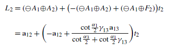
  $$L_1=({\ominus }A_1{\oplus }F_1)t_1=\biggl(\frac{\cot\frac{\alpha_3}{2}\gamma_{12}^{\phantom{O}}\mathbf{a}_{12}+\cot\frac{\alpha _2}{2}\gamma_{13}^{\phantom{O}}\mathbf{a}_{13}}{\cot\frac{\alpha_3}{2}\gamma_{12}^{\phantom{O}}+\cot\frac {\alpha_2}{2}\gamma_{13}^{\phantom{O}}}\biggr)t_1$$

  (7.193)

  as we see from (7.175a), where t ₁∈ℝ is the line parameter.

• 2. The tangent point ⊖ A ₁⊕F ₂ and the vertex a ₁₂=⊖ A ₁⊕A ₂ of the left gyrotranslated gyrotriangle O(⊖ A ₁⊕A ₂)(⊖ A ₁⊕A ₃) form the Euclidean line

  

  (7.194)

  as we see from (7.175b), where t ₂∈ℝ is the line parameter.

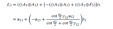
• 3. The tangent point ⊖ A ₁⊕F ₃ and the vertex a ₁₃=⊖ A ₁⊕A ₃ of the left gyrotranslated gyrotriangle O(⊖ A ₁⊕A ₂)(⊖ A ₁⊕A ₃) form the Euclidean line

  

  (7.195)

  as we see from (7.175c), where t ₃∈ℝ is the line parameter.

Since the point P lies on each of the three lines L _k , k=1,2,3, there exist values t _k,0 of the line parameters t _k , k=1,2,3, respectively, such that

(7.196)

where P is given by (7.192).

The system of equations (7.196) was obtained by methods of gyroalgebra, and will be solved below by a common method of linear algebra.

Substituting P from (7.192) into (7.196), and rewriting each of the resulting equations as a linear combination of a ₁₂ and a ₁₃ equals zero, one obtains the following homogeneous linear system of three gyrovector equations

(7.197)

where each coefficient c _ij , i=1,2,3, j=1,2, is a function of the gyrotriangle parameters $\gamma_{12}^{\phantom{O}},\gamma _{13}^{\phantom{O}},\gamma_{23}^{\phantom{O}}$ and α _k , and the six unknowns t _k,0 and m _k , k=1,2,3.

Since the set S={A ₁,A ₂,A ₃} is pointwise independent, the two gyrovectors a ₁₂=⊖ A ₁⊕A ₂ and a ₁₃=⊖ A ₁⊕A ₃ in ${\mathbb{R}}_{s}^{n}$, considered as vectors in ℝⁿ, are linearly independent in ℝⁿ. Hence, each coefficient c _ij in (7.197) equals zero. Accordingly, the three gyrovector equations in (7.197) are equivalent to the following six scalar equations,

$$c_{11}=c_{12}=c_{21}=c_{22}=c_{31}=c_{32}=0$$

(7.198)

for the six unknowns t _k,0 and m _k , k=1,2,3.

An explicit presentation of the resulting system (7.198) reveals that it is slightly nonlinear. However, it is linear in the unknowns t _1,0,t _2,0,t _3,0. Solving three equations of the system for t _1,0,t _2,0,t _3,0, and substituting these into the remaining equations of the system we obtain a system that determines the ratios m ₁/m ₃ and m ₂/m ₃ uniquely, from which convenient (homogeneous) gyrobarycentric coordinates (m ₁:m ₂:m ₃) are obtained. The unique determination of m ₁/m ₃ and m ₂/m ₃ turns out to be

(7.199)

from which two convenient gyrobarycentric coordinates result. These are:

$$(m_1:m_2:m_3)=\biggl(\cot\frac{\alpha_2}{2}\cot\frac{\alpha_3}{2}:\cot\frac{\alpha_1}{2}\cot\frac{\alpha_3}{2}:\cot\frac{\alpha_1}{2}\cot\frac{\alpha_2}{2}\biggr)$$

(7.200)

and, equivalently,

$$(m_1:m_2:m_3)=\biggl(\tan\frac{\alpha_1}{2}:\tan\frac{\alpha_2}{2}:\tan \frac{\alpha_3}{2}\biggr).$$

(7.201)

Formalizing the main result of this section, we have the following theorem:

Theorem 7.22

Let A ₁ A ₂ A ₃ be a gyrotriangle in an Einstein gyrovector space $({\mathbb{R}}_{s}^{n},{\oplus },{\otimes })$. A gyrotrigonometric gyrobarycentric coordinate representation of the gyrotriangle Gergonne gyropoint G _e , Fig. 7.14, p. ??, is given by

$$G_e=\frac{\tan\frac{\alpha_1}{2}\gamma_{_{A_1}}^{\phantom{1}}A_1+\tan \frac{\alpha_2}{2}\gamma_{_{A_2}}^{\phantom{1}}A_2+\tan\frac{\alpha_3}{2}\gamma_{_{A_3}}^{\phantom{O}}A_3}{\tan\frac{\alpha_1}{2}\gamma_{_{A_1}}^{\phantom{1}}+\tan\frac {\alpha_2}{2}\gamma_{_{A_2}}^{\phantom{1}}+\tan \frac{\alpha_3}{2}\gamma_{_{A_3}}^{\phantom{O}}}.$$

(7.202)

Proof

The proof follows immediately from (7.191) and (7.201). □

17 Gyrotriangle Orthogyrocenter

The hyperbolic triangle orthocenter, H, shown in Fig. 7.17, is called in gyrolanguage a gyrotriangle orthogyrocenter.

Fig. 7.17

The orthogyrocenter H of a gyrotriangle A ₁ A ₂ A ₃ in an Einstein gyrovector space $({\mathbb {R}}_{s}^{n},{\oplus },{\otimes })$. Here the orthogyrocenter lies inside its gyrotriangle. There are gyrotriangles with their orthogyrocenter lying out of their gyrotriangles, and there are gyrotriangles that possess no orthogyrocenter, as shown in Figs. 7.18–7.21

Definition 7.23

The orthogyrocenter, H, of a gyrotriangle is the point of concurrency of the gyrotriangle gyroaltitudes.

The three feet, P ₁, P ₂ and P ₃ of the three gyroaltitudes of gyrotriangle A ₁ A ₂ A ₃ in an Einstein gyrovector space $({\mathbb {R}}_{s}^{n},{\oplus },{\otimes })$, shown in Fig. 7.17 for n=2, are given by

(7.203)

The third equation in (7.203) is a copy of (7.119). The first and second equations in (7.203) are obtained from the third one by cyclic permutations of the vertices of gyrotriangle A ₁ A ₂ A ₃.

Gyrotriangle gyroaltitudes are concurrent. The gyroaltitudes of gyrotriangle A ₁ A ₂ A ₃ in an Einstein gyrovector space $({\mathbb{R}}_{s}^{n},{\oplus },{\otimes })$, shown in Fig. 7.17 for n=2, are the gyrosegments A ₁ P ₁, A ₂ P ₂, and A ₁ P ₃. Since gyrosegments in Einstein gyrovector spaces coincide with Euclidean segments, one can employ methods of linear algebra to determine the point of concurrency, that is, the orthogyrocenter, of the three gyroaltitudes of gyrotriangle A ₁ A ₂ A ₃ in Fig. 7.17.

In order to determine the gyrobarycentric coordinates of the gyrotriangle orthogyrocenter in Einstein gyrovector spaces we begin with some gyroalgebraic manipulations that reduce the task we face to a problem in linear algebra.

Let the orthogyrocenter H of gyrotriangle A ₁ A ₂ A ₃ in an Einstein gyrovector space $({\mathbb{R}}_{s}^{n},{\oplus },{\otimes })$, Fig. 7.17, be given in terms of its gyrobarycentric coordinate representation with respect to the set S={A ₁,A ₂,A ₃} of the gyrotriangle vertices by the equation

$$H=\frac{m_1\gamma_{_{A_1}}^{\phantom{1}}A_1+m_2\gamma _{_{A_2}}^{\phantom{1}}A_2+m_3\gamma_{_{A_3}}^{\phantom {O}}A_3}{m_1\gamma_{_{A_1}}^{\phantom{1}}+m_2\gamma _{_{A_2}}^{\phantom{1}}+m_3\gamma_{_{A_3}}^{\phantom{O}}}$$

(7.204)

where the gyrobarycentric coordinates (m ₁:m ₂:m ₃) of H in (7.204) are to be determined.

Left gyrotranslating gyrotriangle A ₁ A ₂ A ₃ by ⊖ A ₁, the gyrotriangle becomes gyrotriangle O(⊖ A ₁⊕A ₂)(⊖ A ₁⊕A ₃), where O=⊖ A ₁⊕A ₁ is the arbitrarily selected origin of the Einstein gyrovector space ${\mathbb {R}}_{s}^{n}$. The gyrotriangle gyroaltitude feet P ₁, P ₂ and P ₃ become, respectively, ⊖ A ₁⊕P ₁, ⊖ A ₁⊕P ₂ and ⊖ A ₁⊕P ₃. These are calculated in (7.205a), (7.205b), (7.205c) below. Employing the Gyrobarycentric Coordinate Representation Gyrocovariance Theorem 4.6, p. 90, we have from Identity (4.29a), p. 91, with X=⊖ A ₁, using the standard gyrotriangle index notation, shown in Fig. 7.17, in Fig. 6.1, p. 128, and in (6.1), p. 127:

(7.205a)

(7.205b)

(7.205c)

Note that, by Definition 4.5, p. 89, the set of points S={A ₁,A ₂,A ₃} is pointwise independent in an Einstein gyrovector space $({\mathbb{R}}_{s}^{n},{\oplus },{\otimes })$. Hence, the two gyrovectors a ₁₂=⊖ A ₁⊕A ₂ and a ₁₃=⊖ A ₁⊕A ₃ in ${\mathbb{R}}_{s}^{n}\subset\mathbb{R}^{n}$ in (7.205a), (7.205b), (7.205c) are linearly independent in ℝⁿ.

Similarly to the gyroalgebra in (7.205a), (7.205b), (7.205c), under a left gyrotranslation by ⊖ A ₁ the orthogyrocenter H in (7.204) becomes

(7.206)

The gyroaltitude of the left gyrotranslated gyrotriangle O(⊖ A ₁⊕A ₂)(⊖ A ₁⊕A ₃) that joins the vertex

$${\ominus }A_1{\oplus }A_1=O=\mathbf{0}$$

(7.207)

with the gyroaltitude foot on its opposing side, P ₁, as calculated in (7.205a),

$${\ominus }A_1{\oplus }P_{1}=\frac{(\gamma_{13}^{\phantom{O}}\gamma _{23}^{\phantom{O}}-\gamma_{12}^{\phantom{O}})\gamma _{12}^{\phantom{O}}\mathbf{a}_{12}+(\gamma_{12}^{\phantom{O}}\gamma_{23}^{\phantom{O}}-\gamma _{13}^{\phantom{O}})\gamma_{13}^{\phantom{O}}\mathbf{a}_{13}}{(\gamma_{13}^{\phantom{O}}\gamma_{23}^{\phantom{O}}-\gamma _{12}^{\phantom{O}})\gamma_{12}^{\phantom{O}}+(\gamma _{12}^{\phantom{O}}\gamma_{23}^{\phantom{O}}-\gamma_{13}^{\phantom{O}})\gamma_{13}^{\phantom{O}}}$$

(7.208)

is contained in the Euclidean line

(7.209)

where t ₁∈ℝ is the line parameter. This line passes through the point $O=\mathbf{0}\in{\mathbb {R}}_{s}^{n}\subset\mathbb{R}^{n}$ when t ₁=0, and it passes through the point ⊖ A ₁⊕P ₁ when t ₁=1.

Similarly to (7.207)–(7.209), the gyroaltitude of the left gyrotranslated gyrotriangle O(⊖ A ₁⊕A ₂)(⊖ A ₁⊕A ₃) that joins the vertex

$${\ominus }A_1{\oplus }A_2=\mathbf{a}_{12}$$

(7.210)

with the gyroaltitude foot on its opposing side, P ₂, as calculated in (7.205b),

$${\ominus }A_1{\oplus }P_{2}=\frac{(\gamma_{12}^{\phantom{O}}\gamma _{13}^{\phantom{O}}-\gamma_{23}^{\phantom{O}})\gamma _{13}^{\phantom{O}}\mathbf{a}_{13}}{(\gamma_{13}^{\phantom{O}}\gamma_{23}^{\phantom{O}}-\gamma _{12}^{\phantom{O}})+(\gamma_{12}^{\phantom{O}}\gamma _{13}^{\phantom{O}}-\gamma_{23}^{\phantom{O}})\gamma_{13}^{\phantom{O}}}$$

(7.211)

is contained in the Euclidean line

(7.212)

where t ₂∈ℝ is the line parameter. This line passes through the point $\mathbf{a}_{12}\in{\mathbb {R}}_{s}^{n}\subset\mathbb{R}^{n}$ when t ₂=0, and it passes through the point ⊖ A ₁⊕P ₂ when t ₂=1.

Similarly to (7.207)–(7.209), and similarly to (7.210)–(7.212), the gyroaltitude of the left gyrotranslated gyrotriangle O(⊖ A ₁⊕A ₂)(⊖ A ₁⊕A ₃) that joins the vertex

$${\ominus }A_1{\oplus }A_3=\mathbf{a}_{13}$$

(7.213)

with the gyroaltitude foot on its opposing side, P ₃, as calculated in (7.205c),

$${\ominus }A_1{\oplus }P_{3}=\frac{(\gamma_{12}^{\phantom{O}}\gamma_{13}^{\phantom{O}}-\gamma _{23}^{\phantom{O}})\gamma_{12}^{\phantom{O}}\mathbf{a}_{12}}{(\gamma_{12}^{\phantom{O}}\gamma_{23}^{\phantom{O}}-\gamma _{13}^{\phantom{O}})+(\gamma_{12}^{\phantom{O}}\gamma _{13}^{\phantom{O}}-\gamma_{23}^{\phantom{O}})\gamma_{12}^{\phantom{O}}}$$

(7.214)

is contained in the Euclidean line

(7.215)

where t ₃∈ℝ is the line parameter. This line passes through the point $\mathbf{a}_{13}\in{\mathbb {R}}_{s}^{n}\subset\mathbb{R}^{n}$ when t ₃=0, and it passes through the point ${\ominus }A_{1}{\oplus }P_{3}\in{\mathbb{R}}_{s}^{n}\subset\mathbb{R}^{n}$ when t ₃=1.

Hence, if the orthogyrocenter H exists, its left gyrotranslated orthogyrocenter, −⊖ A ₁⊕H, given by (7.206), is contained in each of the three Euclidean lines L _k , k=1,2,3, in (7.209), (7.212) and (7.215). Formalizing, if H exists then the point P, (7.206),

$$P={\ominus }A_1{\oplus }H=\frac{m_2\gamma_{12}^{\phantom{O}}\mathbf{a}_{12}+m_3\gamma _{13}^{\phantom{O}}\mathbf{a}_{13}}{m_1+m_2\gamma_{12}^{\phantom{O}}+m_3\gamma_{13}^{\phantom{O}}}$$

(7.216)

lies on each of the lines L _k , k=1,2,3. Imposing the normalization condition m ₁+m ₂+m ₃=1 of gyrobarycentric coordinates, (7.216) can be simplified by means of the resulting equation m ₁=1−m ₂−m ₃, obtaining

$$P={\ominus }A_1{\oplus }H=\frac{m_2\gamma_{12}^{\phantom{O}}\mathbf{a}_{12}+m_3\gamma _{13}^{\phantom{O}}\mathbf{a}_{13}}{1+m_2(\gamma_{12}^{\phantom{O}}-1)+m_3(\gamma_{13}^{\phantom{O}}-1)}.$$

(7.217)

Since the point P lies on each of the three lines L _k , k=1,2,3, there exist values t _k,0 of the line parameters t _k , k=1,2,3, respectively, such that

(7.218)

The kth equation in (7.218), k=1,2,3, is equivalent to the condition that point P lies on line L _k .

The system of equations (7.218) was obtained by methods of gyroalgebra, and will be solved below by a common method of linear algebra.

Substituting P from (7.217) into (7.218), and rewriting each equation in (7.218) as a linear combination of a ₁₂ and a ₁₃ equals zero, one obtains the following linear homogeneous system of three gyrovector equations

(7.219)

where each coefficient c _ij , i=1,2,3, j=1,2, is a function of $\gamma_{12}^{\phantom{O}}$, $\gamma_{13}^{\phantom{O}}$, $\gamma _{23}^{\phantom{O}}$, and the five unknowns m ₂, m ₃, and t _k,0, k=1,2,3.

Since the set S={A ₁,A ₂,A ₃} is pointwise independent, the two gyrovectors a ₁₂=⊖ A ₁⊕A ₂ and a ₁₃=⊖ A ₁⊕A ₃ in ${\mathbb{R}}_{s}^{n}$, considered as vectors in ℝⁿ, are linearly independent in ℝⁿ. Hence, each coefficient c _ij in (7.219) equals zero. Accordingly, the three gyrovector equations in (7.219) are equivalent to the following six scalar equations,

$$c_{11}=c_{12}=c_{21}=c_{22}=c_{31}=c_{32}=0$$

(7.220)

for the five unknowns m ₂,m ₃ and t _k,0, k=1,2,3.

Explicitly, the six scalar equations in (7.220) are equivalent to the following six equations:

(7.221)

The system (7.221) is slightly nonlinear. It is, however, linear in the unknowns t _1,0,t _2,0,t _3,0. Solving three equations of the system for t _1,0,t _2,0,t _3,0, and substituting these into the remaining equations of the system determine the ratios m ₂/m ₁ and m ₃/m ₁ uniquely, from which convenient (homogeneous) gyrobarycentric coordinates (m ₁:m ₂:m ₃) are obtained. A solution of (7.221) is given by (7.222) and (7.224) below:

The values of the line parameters are

(7.222)

where

$$1+2\gamma_{12}^{\phantom{O}}\gamma_{13}^{\phantom{O}}\gamma _{23}^{\phantom{O}}-\gamma_{12}^2-\gamma_{13}^2>0$$

(7.223)

by (6.28), p. 136.

The gyrobarycentric coordinates (m ₁,m ₂,m ₃) are given by

(7.224)

satisfying the normalization condition m ₁+m ₂+m ₃=1, where D is the determinant

(7.225)

or, equivalently,

(7.226)

Following (7.224), convenient gyrobarycentric coordinates of the gyrotriangle orthogyrocenter H are given by the equation

$$(m_1:m_2:m_3)=(C_{12}C_{13}:C_{12}C_{23}:C_{13}C_{23})$$

(7.227)

or, equivalently, by the equation

$$(m_1:m_2:m_3)=\biggl(\frac{C_{12}}{C_{23}}:\frac{C_{12}}{C_{13}}:1\biggr)$$

(7.228)

where

(7.229)

Accordingly, the gyrobarycentric coordinate representation of the orthogyrocenter H of gyrotriangle A ₁ A ₂ A ₃ with respect to the set of the gyrotriangle vertices is given by the equation

$$H=\frac{C_{12}C_{13}\gamma_{A_1}^{\phantom{O}}A_1+C_{12}C_{23}\gamma_{A_2}^{\phantom{O}}A_2+C_{13}C_{23}\gamma_{A_3}^{\phantom{O}}A_3}{C_{12}C_{13}\gamma_{A_1}^{\phantom{O}}+C_{12}C_{23}\gamma_{A_2}^{\phantom{O}}+C_{13}C_{23}\gamma_{A_3}^{\phantom{O}}}.$$

(7.230)

Substituting from (7.147), p. ??, into (7.229), we have

(7.231)

Hence, the gyrobarycentric coordinates of H in (7.228) can be written as

$$(m_1:m_2:m_3)=\biggl(\frac{\tan\alpha_1}{\tan\alpha_3}:\frac {\tan\alpha_2}{\tan\alpha_3}:1\biggr)$$

(7.232)

which are, in turn, equivalent to the gyrobarycentric coordinates

$$(m_1:m_2:m_3)=(\tan\alpha_1:\tan\alpha_2:\tan\alpha_3).$$

(7.233)

Interestingly, the gyrotrigonometric gyrobarycentric coordinates (7.233) of the gyrotriangle orthogyrocenter H are identical in form with trigonometric barycentric coordinates of the triangle orthocenter in Euclidean geometry, as we see from [29].

Following (7.227) and the definition, Definition (4.5), p. 89, of the constant m ₀, (4.27), of a point P with a gyrobarycentric representation, the constant m ₀ of the gyrotriangle orthogyrocenter H in (7.230) with respect to the set of the gyrotriangle vertices is given by the equation

(7.234)

where f ₁ and f ₂ are factors given by

(7.235)

Since f ₁>0, by (6.23), p. 135, the constant $m_{0}^{2}$ in (7.234) is positive, zero, or negative if and only if $f_{1}^{2}+f_{2}$ is positive, zero, or negative, respectively. Hence, equivalently, the constant $m_{0}^{2}$ in (7.234) is positive, zero, or negative if and only if $f_{1}^{4}-f_{2}^{2}$ is positive, zero, or negative, respectively. Expressing of gamma factors of sides of gyrotriangle A ₁ A ₂ A ₃ in terms of the gyrotriangle gyroangles by (7.142), p. ??, we have

(7.236)

where Q is a positive valued function of cos α _k , k=1,2,3.

Hence, the constant $m_{0}^{2}$ in (7.234) is positive, zero, or negative if and only if f ₃ is positive, zero, or negative, respectively, where

(7.237)

According to Corollary 4.9, p. 93, if $m_{0}^{2}>0$ then gyrotriangle A ₁ A ₂ A ₃ possesses a orthogyrocenter H. The orthogyrocenter H lies in the interior of gyrotriangle A ₁ A ₂ A ₃ if and only if gyrobarycentric coordinates of H are all positive or all negative. The gyrotriangle A ₁ A ₂ A ₃ does not have a orthogyrocenter H when $m_{0}^{2}\le0$ in (7.234). When $m_{0}^{2}=0$, the point H lies on the boundary of the ball ${\mathbb{R}}_{s}^{n}$, and when $m_{0}^{2}<0$ the point H lies outside of the ball, as shown in Figs. 7.18–7.21. Indeed,

• 1. f ₃>0 for gyrotriangle A ₁ A ₂ A ₃ in Figs. 7.17, p. ??, and 7.18–7.19

  Fig. 7.18

  

  The gyroaltitudes, and the orthogyrocenter H, of a gyrotriangle A ₁ A ₂ A ₃ in an Einstein gyrovector space. Case I: The orthogyrocenter H lies inside the acute gyrotriangle. Gyrobarycentric coordinates (m ₁:m ₂:m ₃) of the orthogyrocenter H relative to the set {A ₁,A ₂,A ₃} of the gyrotriangle vertices, given by (7.233), are all positive so that $m_{0}^{2}>0$ in (7.234), in agreement with Corollary 4.10, p. 94

  Fig. 7.19

  

  The gyroaltitudes, and the orthogyrocenter H, of a gyrotriangle A ₁ A ₂ A ₃ in an Einstein gyrovector space. Case II: The orthogyrocenter H lies outside the obtuse gyrotriangle. One of the gyrobarycentric coordinates (m ₁:m ₂:m ₃) of the orthogyrocenter H relative to the set {A ₁,A ₂,A ₃} of the gyrotriangle vertices, given by (7.233), is negative and the other two are positive, in agreement with Corollary 4.9

• 2. f ₃=0 for gyrotriangle A ₁ A ₂ A ₃ in Fig. 7.20, p. ??; and

  Fig. 7.20

  

  A gyrotriangle A ₁ A ₂ A ₃ that does not possess an orthogyrocenter H in an Einstein gyrovector plane $({\mathbb{R}}_{s}^{2},{\oplus },{\otimes })$. The point H∈ℝⁿ lies on the boundary of the ball ${\mathbb{R}}_{s}^{n}\subset \mathbb{R}^{n}$. Accordingly $m_{0}^{2}=0$ in (7.234), in agreement with Corollary 4.9, p. 93

• 3. f ₃<0 for gyrotriangle A ₁ A ₂ A ₃ in Fig. 7.21, p. ??

  Fig. 7.21

  

  A gyrotriangle A ₁ A ₂ A ₃ that does not possess an orthogyrocenter H in an Einstein gyrovector plane $({\mathbb{R}}_{s}^{2},{\oplus },{\otimes })$. The point H∈ℝⁿ lies outside of the ball ${\mathbb {R}}_{s}^{n}\subset\mathbb{R}^{n}$. Accordingly $m_{0}^{2}<0$ in (7.234), in agreement with Corollary 4.9, p. 93

Formalizing the main result of this section, we have the following theorem:

Theorem 7.24

(The Orthogyrocenter) Let S={A ₁,A ₂,A ₃} be a pointwise independent set of three points in an Einstein gyrovector space $({\mathbb{R}}_{s}^{n},{\oplus },{\otimes })$. The orthogyrocenter H, see Figs. 7.18 – 7.21, of gyrotriangle A ₁ A ₂ A ₃ has the gyrobarycentric coordinate representation

$$H=\frac{m_1\gamma_{_{A_1}}^{\phantom{1}}A_1+m_2\gamma _{_{A_2}}^{\phantom{1}}A_2+m_3\gamma_{_{A_3}}^{\phantom {O}}A_3}{m_1\gamma_{_{A_1}}^{\phantom{1}}+m_2\gamma _{_{A_2}}^{\phantom{1}}+m_3\gamma_{_{A_3}}^{\phantom{O}}}$$

(7.238)

with respect to the set S={A ₁,A ₂,A ₃}, with gyrotrigonometric gyrobarycentric coordinates given by each of the two equations

$$(m_1:m_2:m_3)=(\tan\alpha_1:\tan\alpha_2:\tan\alpha_3)$$

(7.239)

and

(7.240)

The existence of the gyrotriangle orthogyrocenter H is determined by the squared orthogyrocenter constant $m_{0}^{2}$ with respect to the set of the gyrotriangle vertices,

(7.241)

The gyrotriangle orthogyrocenter H exists if and only if $m_{0}^{2}>0$. Furthermore, the gyrotriangle orthogyrocenter H lies on the interior of its gyrotriangle if and only if tan α ₁>0, tan α ₂>0 and tan α ₃>0 or, equivalently, if and only if the gyrotriangle is acute, see Figs. 7.18 – 7.21.

The gyrotrigonometric gyrobarycentric coordinates (7.239) remain invariant in form under the Euclidean limit s→∞, resulting in the following corollary of Theorem 7.24:

Corollary 7.25

(The Orthocenter) Let S={A ₁,A ₂,A ₃} be a pointwise independent set of three points in a Euclidean vector space ℝⁿ. The orthocenter H of triangle A ₁ A ₂ A ₃ has the barycentric coordinate representation

$$H=\frac{m_1A_1+m_2A_2+m_3A_3}{m_1+m_2+m_3}$$

(7.242)

with respect to the set S={A ₁,A ₂,A ₃}, with trigonometric barycentric coordinates given by

$$(m_1:m_2:m_3)=(\tan\alpha_1:\tan\alpha_2:\tan\alpha_3).$$

(7.243)

18 The Gyrodistance Between O and I

Let O and I be the circumgyrocenter and ingyrocenter of a gyrotriangle A ₁ A ₂ A ₃ in an Einstein gyrovector space $({\mathbb{R}}_{s}^{n},{\oplus },{\otimes })$. Their gyrobarycentric coordinate representations with respect to the set S={A ₁,A ₂,A ₃} are, by (7.18) and (7.20), p. ??,

$$O=\frac{m_1^\prime\gamma_{_{A_1}}^{\phantom{1}}A_1+m_2^\prime\gamma_{_{A_2}}^{\phantom{1}}A_2+m_3^\prime\gamma_{_{A_3}}^{\phantom{1}}A_3}{m_1^\prime\gamma_{_{A_1}}^{\phantom{1}}+m_2^\prime\gamma_{_{A_2}}^{\phantom{1}}+m_3^\prime\gamma_{_{A_3}}^{\phantom{1}}},$$

(7.244a)

where the gyrobarycentric coordinates $m_{k}^{\prime}$, k=1,2,3, are given by

(7.244b)

and, by (7.75), p. ??, and Theorem 7.12, p. ??,

$$I=\frac{m_1\gamma_{_{A_1}}^{\phantom{1}}A_1+m_2\gamma _{_{A_2}}^{\phantom{1}}A_2+m_3\gamma_{_{A_3}}^{\phantom {O}}A_3}{m_1\gamma_{_{A_1}}^{\phantom{1}}+m_2\gamma _{_{A_2}}^{\phantom{1}}+m_3\gamma_{_{A_3}}^{\phantom{O}}},$$

(7.245a)

where the gyrobarycentric coordinates m _k , k=1,2,3, are given by

(7.245b)

Hence, by (4.121), p. 113,

(7.246)

where, by (4.118b) and (4.119b), p. 112, m ₀>0 and $m_{0}^{\prime}>0$ are given by

(7.247)

noting that always $m_{0}^{2}>0$; and that $(m_{0}^{\prime})^{2}>0$ if and only if gyrotriangle A ₁ A ₂ A ₃ possesses a circumgyrocenter.

Substituting (7.244b) and (7.245b) into (7.246) and squaring, one obtains $\gamma_{{\ominus }O{\oplus }I}^{2}$ expressed in terms of the gyrotriangle gyroangles α _k , k=1,2,3. Substituting the latter, in turn, into the identity, (1.9), p. 5,

$$\|{\ominus }O{\oplus }I\|^2=s^2\frac{\gamma_{{\ominus }O{\oplus }I}^{2}-1}{\gamma_{{\ominus }O{\oplus }I}^{2}},$$

(7.248)

we finally obtain the desired gyrodistance,

(7.249)

Eliminating the factor $s^{2}\cos\frac{\alpha_{1}+\alpha_{2}+\alpha_{3}}{2}$ between (7.249) and (7.35), p. ??, we obtain the result (7.250) of the following theorem:

Theorem 7.26

Let α _k , k=1,2,3, O and I be the gyroangles, circumgyrocenter and ingyrocenter of a gyrotriangle A ₁ A ₂ A ₃ in an Einstein gyrovector space $({\mathbb {R}}_{s}^{n}{\oplus },{\otimes })$. Then,

(7.250)

Interestingly, Equation (7.250) remains invariant in form under the Euclidean limit s→∞, so that the equation is valid in Euclidean geometry as well. However, for application in Euclidean geometry (7.250) can be simplified, owing to the fact that triangle angle sum in π.

Indeed, under the condition

$$\alpha_1+\alpha_2+\alpha_3=\pi,$$

(7.251a)

we have the trigonometric identities similar to (7.22b), p. ??,

(7.251b)

Hence, we obtain the following corollary of Theorem 7.26:

Corollary 7.27

Let α _k , k=1,2,3, O and I be the angles, circumcenter and incenter of a triangle A ₁ A ₂ A ₃ in a Euclidean space ℝⁿ. Then,

(7.252)

19 Problems

Problem 7.1

The constant of a Gyrobarycentric Coordinate Representation:

Derive (7.11), p. ??, from (7.10) and (7.3).

Problem 7.2

Gyrotrigonometric Substitutions:

Substitute from (7.13) into (7.10) to obtain (7.14), p. ??.

Problem 7.3

Gyrotrigonometric Substitutions:

Derive the gyrotrigonometric representation (7.34), p. ??, of the gyrotriangle circumgyroradius R by expressing the gamma factors in (7.29), p. ??, in terms of the gyrotriangle gyroangles α _k , k=1,2,3, by means of (6.33), p. 137.

Remarkably, this task in gyrotrigonometry can straightforwardly be performed by Mathematica, a software for computer algebra, using commands that manipulate common trigonometric identities like TrigToExp, ExpToTrig, TrigReduce and TrigFactor.

Problem 7.4

Show that (7.40), p. ??, holds when the three points A ₁, A ₂ and A ₃ in Theorem 7.5 are not distinct.

Problem 7.5

A Gyrotriangle Gyroangle Inequality:

Employ (7.13), p. ??, to derive Inequality (7.17), p. ??, from Inequality (7.12), p. ??.

Problem 7.6

Linear Algebra:

Provide the missing technical details in the derivation of (7.95), p. ??, from (7.89), p. ??.

Problem 7.7

Gyrotriangle Gyrotrigonometric Identities:

Verify the gyrotriangle gyrotrigonometric identities in (7.149)–(7.151), p. ??.

Problem 7.8

Gyrotrigonometric Substitutions:

Derive (7.187), p. ??, by substitutions from (7.185), p. ??, and from (7.142), p. ??.

Problem 7.9

Gyrotrigonometric Substitutions:

Derive the first two equations in (7.189), p. ??, from (7.188).

Problem 7.10

Derive (7.190), p. ??, from (7.189).

Problem 7.11

Gyrotriangle Orthogyrocenter:

Solve the system (7.221), p. ??, and hence derive the gyrobarycentric coordinates (7.224).

Problem 7.12

Gyrotrigonometric Substitutions:

By substitutions from (6.33), p. 137, derive the gyrotrigonometric condition f ₃ in (7.237), p. ??, that determines whether the orthogyrocenter H of gyrotriangle A ₁ A ₂ A ₃ exists.

Problem 7.13

Gyrotrigonometric Substitutions:

By substitutions from (7.244b) and (7.245b) into (7.246) and squaring, express $\gamma_{{\ominus }O{\oplus }I}^{2}$ in terms of the gyroangles α _k , k=1,2,3, of the reference gyrotriangle A ₁ A ₂ A ₃. Furthermore, substitute the latter into (7.248) to obtain the squared gyrodistance ‖⊖ O⊕I‖² in (7.249), p. ??.

References

Bottema, O.: On the medians of a triangle in hyperbolic geometry. Can. J. Math. 10, 502–506 (1958)
Demirel, O., Soyturk, E.: The hyperbolic Carnot theorem in the Poincaré disc model of hyperbolic geometry. Novi Sad J. Math. 38(2), 33–39 (2008)
Honsberger, R.: Episodes in Nineteenth and Twentieth Century Euclidean Geometry. New Mathematical Library, vol. 37, p. 174. Math. Assoc. Am., Washington (1995)
Kelly, P.J., Matthews, G.: The Non-Euclidean, Hyperbolic Plane. Universitext, p. 333. Springer, New York (1981). Its structure and consistency
Kimberling, C.: Clark Kimberling’s Encyclopedia of Triangle Centers—ETC. http://faculty.evansville.edu/ck6/encyclopedia/ETC.html (2010)
Maor, E.: Trigonometric Delights, p. 236. Princeton University Press, Princeton (1998)
Sonmez, N.: A trigonometric proof of the Euler theorem in hyperbolic geometry. Algebras Groups Geom. 26(1), 75–79 (2009)
Vermeer, J.: A geometric interpretation of Ungar’s addition and of gyration in the hyperbolic plane. Topol. Appl. 152(3), 226–242 (2005)
Author information
Authors and Affiliations
Corresponding author
Rights and permissions
Copyright information
© 2010 Springer Science+Business Media B.V.
About this chapter
Cite this chapter
Ungar, A.A. (2010). Gyrotriangle Gyrocenters. In: Hyperbolic Triangle Centers. Fundamental Theories of Physics, vol 166. Springer, Dordrecht. https://doi.org/10.1007/978-90-481-8637-2_7
Download citation
DOI: https://doi.org/10.1007/978-90-481-8637-2_7
Publisher Name: Springer, Dordrecht
Print ISBN: 978-90-481-8636-5
Online ISBN: 978-90-481-8637-2
eBook Packages: Physics and AstronomyPhysics and Astronomy (R0)