In this chapter we will introduce the domain decomposition method (DD, in short). In its most common version, DD can be used in the framework of any discretization method for partial differential equations (such as, e.g. finite elements, finite volumes, finite differences, or spectral element methods) to make their algebraic solution more efficient on parallel computer platforms. In addition, DD methods allow the reformulation of any given boundary-value problem on a partition of the computational domain into subdomains. As such, it provides a very convenient framework for the solution of heterogeneous or multiphysics problems, i.e. those that are governed by differential equations of different kinds in different subregions of the computational domain.
These keywords were added by machine and not by the authors. This process is experimental and the keywords may be updated as the learning algorithm improves.
In this chapter we will introduce the domain decomposition method (DD, in short). In its most common version, DD can be used in the framework of any discretization method for partial differential equations (such as, e.g. finite elements, finite volumes, finite differences, or spectral element methods) to make their algebraic solution more efficient on parallel computer platforms. In addition, DD methods allow the reformulation of any given boundary-value problem on a partition of the computational domain into subdomains. As such, it provides a very convenient framework for the solution of heterogeneous or multiphysics problems, i.e. those that are governed by differential equations of different kinds in different subregions of the computational domain.
The basic idea behind DD methods consists in subdividing the computational domain Ω, on which a boundary-value problem is set, into two or more subdomains on which discretized problems of smaller dimension are to be solved, with the further potential advantage of using parallel solution algorithms. More in particular, there are two ways of subdividing the computational domain into subdomains: one with disjoint subdomains, the others with overlapping subdomains (for an example, see Fig. 18.1). Correspondingly, different DD algorithms will be set up.
Fig. 18.1
Two examples of subdivision of the domain Ω, with and without overlap
L being a generic second order elliptic operator, whose weak formulation reads
$${find\ u\ \in\ V = H ^1_0(\Omega)}:{a(u,v)=(f,v)\ \forall\ v\ \in\ V},$$
(18.2)
being a(.,.)the bilinear form associated with L.
1.1 18.1.1 Schwarz method
Consider a decomposition of the domain Ω in two subdomains Ω1 and Ω2 such that \({\overline \Omega = \overline \Omega_1\cup \overline \Omega_2}\), Ω1 ⋂Ω2 = Ω12 ≠ ∅ (see Fig. 18.1) and let Γi = ∂Ωi\ (∂Ω n∂Ωi).
Consider the following iterative method. Given u(20) on Γ1 solve the following problems for k ≥ 1:
In the case in which one chooses u1(k)on Γ2 in (18.4) the method is named multiplica¬tive Schwarz, whereas that in which we choose u(1k-1) is named additive Schwarz. The reason will be clarified in Sect.18.6. We have thus two elliptic boundary-value prob¬lems with Dirichlet conditions for the two subdomains Ω1 and Ω2, and we would like the two sequences {u1(k) } and {u2(k) } to converge to the restrictions of the solution u of problem (18.1), that is
It can be proven that the Schwarz method applied to problem (18.1) always converges, with a rate that increases as the measure |Ω12| of the overlapping region Ω12 increases. Let us show this result on a simple one-dimensional case.
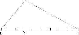
Example 18.1. Let Ω= (a,b) and let γ1,γ2∈ (a,b) be such that a <γ2<γ1< b (see Fig. 18.2). The two problems (18.3) and (18.4) become:
$$\left\{ {\begin{array}{*{20}{l}}
{Lu_2^{\left( k \right)} = f\quad \quad \quad a < x < {\gamma _1},} \\
{u_2^{\left( k \right)} = u_2^{\left( {k - 1} \right)},\quad \quad \,x = {\gamma _1},} \\
{u_2^{\left( k \right)} = 0\quad \quad \quad \;\;\;x = a,}
\end{array}} \right.$$
To show that this scheme converges, let us bound ourselves to the simpler problem
$$\left\{ {\begin{array}{*{20}{l}}
{ - u''\left( x \right) = 0\quad \quad \quad a < x < b,} \\
{u\left( a \right) = u\left( b \right) = 0,}
\end{array}} \right.$$
(18.7)
that is the model problem (18.1) with L = —d2/dx2 and f = 0, whose solution clearly is u = 0 in (a,b). This is not restrictive since at every step the error: u — u1(k)k in Ω1, u — u2(k)in Ω2, satisfies a problem like (18.5)-(18.6) with null forcing term.
Let k= 1; since (u1(1) )" = 0,u(11) (x) is a linear function; moreover, it vanishes at x = a and takes the value u2(0) at x = γ1. As we know the value of u1(1) at γ2, we can solve the problem (18.6) which, in its turn, features a linear solution. Then we proceed in a similar manner. In Fig. 18.2 we show a few iterations: we clearly see that the method converges, moreover the convergence rate reduces as the length of the interval (γ2, γ1) gets smaller.
At each iteration the Schwarz iterative method (18.3)–(18.4) requires the solution of two subproblems with boundary conditions of the same kind as those of the original problem: indeed, by starting with a Dirichlet boundary-value problem in Ω we end up with two subproblems with Dirichlet conditions on the boundary of Ω1 and Ω2. Should the differential problem (18.1) had been completed by a Neumann boundary condition on the whole boundary ∂Ω, we would have been led to the solution of a mixed Dirichlet-Neumann boundary-value problem on either subdomain Ω1 and Ω2.
1.2 18.1.2 Dirichlet-Neumann method
Let us partition the domain Ω in two disjoint subdomains (as in Fig. 18.1): let then Ω1 and Ω2 be two subdomains providing a partition of Ω,i.e. \({\overline \Omega_1\cup \overline \Omega_2 =\overline \Omega ,\overline \Omega_1\cap \overline \Omega_2=\Gamma}\) and Ω1 n Ω2 = ∅. We denote by ni the outward unit normal vector to Ωi and will use the following notational convention: n = n1 = — n2.
The following result holds (for its proof see [QV99]):
Theorem 18.1 (of equivalence).The solution u of problem (18.1) is such that uΩi= uifor i = 1,2, where ui is the solution to the problem
on Γ, having denoted with ∂ /∂nL the conormal derivative (see (3.34)).
Thanks to this result we could split problem (18.1) by assigning the interface con ditions (18.9)-(18.10) the role of “boundary conditions” for the two subproblems on the interface Γ. In particular, we can set up the following Dirichlet-Neumann (DN) iterative algorithm : given u2(0) on Γ, for k ≥ 1 solve the problems:
$$\left\{ {\begin{array}{*{20}{l}}
{Lu_1^{\left( k \right)} = f\quad \quad in\,{\Omega _2},} \\
{\frac{{\partial u_2^{\left( k \right)}}}{{\partial n}} = \frac{{\partial u_1^{\left( k \right)}}}{{\partial n}}\quad on\,\Gamma ,} \\
{u_2^{\left( k \right)} = 0\quad \quad \quad on\,\partial {\Omega _1}\backslash \Gamma ,}
\end{array}} \right.$$
(18.12)
Condition (18.9) has generated a Dirichlet boundary condition on Γ for the subprob-lem in Ω1 whereas (18.10) has generated a Neumann boundary condition on Γ for the subproblem in Ω2.
Differently than Schwarz’s method, the DN algorithm yields a Neumann boundary-value problem on the subdomain Ω2. Theorem 18.1 guarantees that when the two sequences {u1(k)} and {u2(k) } converge, then their limit will be perforce the solution to the exact problem (18.1). The DN algorithm is therefore consistent. Its convergence however is not always guaranteed, as we can see on the following simple example.
Example 18.2. Let Ω = (a,b), γ∈ (a,b),L= —d2/dx2 andf = 0. At every k ≥ 1 the DN algorithm generates the two subproblems:
$$\left\{ {\begin{array}{*{20}{l}}
{ - {{\left( {u_1^{\left( k \right)}} \right)}^{\prime \prime }} = 0\quad a < x < \gamma ,} \\
{u_1^{\left( k \right)} = 0\quad \quad \quad x = a,} \\
{u_1^{\left( k \right)} = u_2^{\left( {k - 1} \right)},\quad x = \gamma ,}
\end{array}} \right.$$
(18.13)
$$\left\{ {\begin{array}{*{20}{l}}
{ - {{\left( {u_1^{\left( k \right)}} \right)}^{\prime \prime }} = 0\quad \quad \gamma < x < b,} \\
{{{\left( {u_1^{\left( k \right)}} \right)}^\prime } = \left( {u_1^{\left( k \right)}} \right),\quad x = \gamma ,} \\
{u_2^{\left( k \right)} = 0,\quad \quad \quad \quad x = b.}
\end{array}} \right.$$
(18.14)
Proceeding as done in Example 18.1, we can prove that the two sequences converge only if γ> (a+b)/2, as shown graphycally in Fig. 18.3.
Fig. 18.3
Example of converging (left) and diverging (right) iterations for the DN method in 1D
In general, for a problem in arbitrary dimension d > 1, the measure of the "Dirich-let" subdomain Ω1 must be larger than that of the "Neumann" one Ω2 in order to guarantee the convergence of (18.11)-(18.12). This however yields a severe constraint to fulfill, especially if several subdomains will be used.
To overcome such limitation, a variant of the DN algorithm can be set up by replacing the Dirichlet condition (18.11)2 in the first subdomain by
that is by introducing a relaxation which depends on a positive parameter θ. In such a way it is always possible to reduce the error between two subsequent iterates.
In the case displayed in Fig. 18.3 we can easily verify that, by choosing
the algorithm converges to the exact solution in a single iteration.
More in general, it can be proven that in any dimension d≥1, there exists a suitable value θmax < 1 such that the DN algorithm converges for any possible choice of the relaxation parameter θ in the interval (0, θmax).
1.3 18.1.3 Neumann-Neumann algorithm
Consider again a partition of Ω into two disjoint subdomains and denote by λ the (unknown) value of the solution u at their interface Γ. Consider the following iterative algorithm: for any given λ(0) on Γ, for k ≥ 0 and i= 1,2 solve the following problems:
where θ is a positive acceleration parameter, while σ1 and σ2 are two positive coef¬ficients such that σ1+ σ2 = 1. This iterative algorithm is named Neumann-Neumann (NN). Note that in the first stage (18.17) we care about the continuity on Γ of the func¬tions u1(k+1)and u2(k+1) but not that of their derivatives. The latter are addressed in the second stage (18.18), (18.19) by means of the correcting functions ψ1(k+1) and ψ2(k+1).
1.4 18.1.4 Robin-Robin algorithm
At last, we consider the following iterative algorithm, named Robin-Robin (RR). For every k ≥ 0 solve the following problems:
where u0 is assigned and γ1, γ2 are non-negative acceleration parameters that satisfy γ1+γ2 >0. Aiming at the algorithm parallelization, in (18.21) we could use u1(k) instead of u1(k+1) , provided in such a case an initial value for u01 is assigned as well.
2 18.2 Multi-domain formulation of Poisson problem and interface conditions
In this section, for the sake of exposition, we choose L = —Δ and consider the Poisson problem with homogeneous Dirichlet boundary conditions (3.13). Generalization to an arbitrary second order elliptic operator with different boundary conditions is in order.
In the case addressed in Sect. 18.1.2 of a domain partitioned into two disjoint sub-domains, the equivalence Theorem 18.1 allows the following multidomain formulation of problem (18.1), in which ui = u|Ωi, i = 1,2:
We denote again by λ the unknown value of the solution u of problem (3.13) on the interface Γ, that is λ = u|Γ. Should we know a priori the value λ on Γ, we could solve the following two independent boundary-value problems with Dirichlet condition on Γ (i = 1,2):
respectively. Note that the functions w*i depend solely on the source data f, while u0i solely on the value λ on Γ, henceforth we can write w*i = Gif and u0i = Hiλ. Both operators Gi and Hi are linear; Hi is the so-called harmonic extension operator of λ on the domain Ωi.
By a formal comparison of problem (18.22) with problem (18.23), we infer that the equality
$$u_i = w^*_i + u^0_i , i = 1,2,$$
holds iff the condition (18.22)6 on the normal derivatives on Γ is satisfied, that is iff
is called local Steklov-Poincaré operator. Note that S, S1 and S2 operate between the trace space
$$\Lambda = \lbrace\ \mu\ |\ \exists v\ \in\ V : \mu = v |_ \Gamma\rbrace$$
(18.30)
(that is \({H^{1/2}_{00}(\Gamma)}\), see [QV99]), and its dual ∧', whereas χ ∈ ∧'.
Example 18.3. With the aim of providing a practical (elementary) example of operator S, let us consider a simple one-dimensional problem. Let Ω = (a,b) ⊂; ℝ as shown in Fig. 18.4 and Lu = —u". By subdividing Ω in two disjoint subdomains, the interface Γ reduces to a single point γ ∈ (a, b), and the Steklov-Poincaré operator S becomes
2.2 18.2.2 Equivalence between Dirichlet-Neumann and Richardson methods
The Dirichlet-Neumann (DN) method introduced in Sect. 18.1.2 can be reinterpreted as a (preconditioned) Richardson method for the solution of the Steklov-Poincaré in terface equation. To check this statement, consider again, for the sake of simplicity, a domain Ω partitioned into two disjoint subdomains Ω1 and Ω2 with interface Γ.
Then we re-write the DN algorithm (18.11), (18.12), (18.15) in the case of the operator L = − Δ: for a given λ0, for k ≥ 1 solve:
In particular \({{u^{(k)}_2}_{|\Gamma}=(u^{(k)}_2-G_2f_2)_{|\Gamma }}\). Since the operator Si (18.29) maps a Dirichlet data to a Neumann data on Γ, its inverse \({S^{-1}_i}\) transforms a Neumann data in a Dirichlet one on Γ.
Otherwise said, \({S^{-1}_2 \eta = w_{2_{|\Gamma}}}\), where w2 is the solution of
that is (18.34). The preconditioned DN operator is therefore S2−1S = I +S-21S1.
Using an argument similar to that used for the proof of Theorem 18.2, also the Neumann-Neumann (NN) algorithm (18.17)–(18.19) can be interpreted as a precon ditioned Richardson algorithm
$$P_{NN} (\lambda^{(k)} - \lambda^{(k-1)}) = \theta (\chi - S \lambda^{(k-1)}),$$
this time the preconditioner being PNN = (D1S1−D1 + D2S2D2)−1 where Di is a diagonal matrix whose entries are equal to σi. Note that the preconditioned operator becomes (if Di = I) S2−1S1 + 2I + (S2−1S1)−1.
Consider at last the Robin-Robin iterative algorithm (18.20)–(18.21). Denoting by \({\mu^{(k)}_i \in \Lambda}\) the approximation at step k of the trace of \({u^{(k)}_i}\) on the interface Γ,i= 1,2, it can be proven that (18.20)–(18.21) is equivalent to the following alternating direction (ADI) algorithm:
where iΛ: Λ → Λ' here denotes the Riesz isomorphism between the Hilbert space Λ and its dual Λ' (see (2.5)).
Should, for a convenient choice of the two parameters γ1 and γ2, the algorithm converge
to two limit functions µ1 and µ2, then µ1 = µ2 = λ, the latter function being the solution
to the Steklov-Poincaré equation (18.26).
Remark 18.1. In the Dirichlet-Neumann algorithm, the value λ of the solution u at the interface Γ is the principal unknown. Once it has been determined, we can use it as Dirichlet data to recover the original solution in the whole domain. Alternatively, one could use the normal derivative \({\eta = {\partial u \over \partial n}}\) on Γ as principal unknown (or, for a more general partial differential operator, the conormal derivative - or flux). By proceeding as above, we can show that η satisfies the new Steklov-Poincaré equation
The so-called FETI algorithms (see Sect. 18.5.4) are examples of iterative algo¬rithms designed for the solution of problems like (18.38). The FETI preconditioner is PFETI = S1+ S2, hence the preconditioned FETI operator is \((S_1+S_2)(S^{-1}_1+S^{-1}_2)\).
3 18.3 Multidomain formulation of the finite element approximation of the Poisson problem
What seen thus far can be regarded as propedeutical to numerical solution of boundary-value problems. In this section we will see how the previous ideas can be reshaped in the framework of a numerical discretization method. Although we will only address the case of finite element discretization, this is however not restrictive. We refer, e.g., to [CHQZ07] and [TW05] for the case of spectral or spectral element discretizations and to [Woh01] for discretization based on DG and mortar methods.
Consider the Poisson problem (3.13), its weak formulation (3.18) and its Galerkin finite element approximation (4.40) on a triangulation Th. Recall that \({V_h = {\buildrel \circ \over X}^r_h = \lbrace \nu_h \in X^r_h : \nu_h |_{\partial \Omega} =0 \rbrace}\) is the space of finite element functions of degree r vanishing on ∂Ω, whose basis is \({\lbrace \varphi_j \rbrace^{N_h}_{j=1}}\) (see Sect. 4.5.1).
For the finite element nodes in the domain Ω we consider the following partition: let \({\lbrace x^{(1)}_j , 1\leq j \leq N_1 \rbrace}\) be the nodes located in the subdomain \(\Omega_1,{\lbrace x^{(2)}_j , 1\leq j \leq N_2 \rbrace}\) those in Ω2 and, finally, \({\lbrace x^{(\Gamma)}_j , 1\leq j \leq N_{\Gamma} \rbrace}\) those lying on the interface Γ. Let us split the basis functions accordingly: \({\varphi^{(1)}_j}\) will denote those associated to the nodes \({x^{(1)}_j}\), \({\varphi^{(2)}_j}\) those associated with the nodes \({x^{(2)}_j}\), and \({\varphi^{(\Gamma)}_j}\) those associated with the nodes \({x^{(\Gamma)}_j}\) lying on the interface. This yields
$$a_i (v,w) = \int_{\Omega_i}\ \nabla_v . \nabla_w d \Omega \quad \forall_v, w \epsilon V, i = 1,2$$
be the restriction of the bilinear form a (.,.) to the subdomain Ωi and define Vi, h = {v ∈ H1(Ωi) | v = 0 on ∂Ωi\Γ} (i = 1,2). Similarly we set Fi(v) = ∫ΩifvdΩ and denote by \({u^{(i)}_h =u_{h_{|_{\Omega_{i}}}}}\) the restriction of uh to the subdomain Ωi, with i= 1,2. Problem (18.41) can be rewritten in the equivalent form: find \({u^{(1)}_h \in V_{1,h}, u^{(2)}_h \in V_{2,h}}\) such that
The interface continuity condition (18.22)5 is automatically satisfied thanks to the continuity of the functions \({u^{(i)}_h}\) Moreover, equations (18.42)1-(18.42)3 correspond to the finite element discretization of equations (18.22)1 -(18.22)6, respectively. In particular, the third of equations (18.42) must be regarded as the discrete counterpart of condition (18.22)6 expressing the continuity of normal derivatives on Γ.
Let us expand the solution uh with respect to the basis functions Vh
From now on, the nodal values \({u_h(x^{(\alpha)}_j)}\), for α = 1,2,Γ and j = 1,...,Nα, which are the expansion coefficients, will be indicated with the shorthand notation \({u^{(\alpha)}_j}\).
having set \({A_{\Gamma \Gamma}=\Big ( A^{(1)}_{\Gamma \Gamma}+A^{(2)}_{\Gamma \Gamma} \Big)}\) and \({{\bf f}_\Gamma = {\bf f}^\Gamma_1 + {\bf f}^\Gamma_2}\) (18.47) is nothing but a blockwise representation of the finite element system (4.46), the blocks being determined by the partition (18.45) of the vector of unknowns.
More precisely, the first and second equations of (18.46) are discretizations of the given Poisson problems in Ω1 and Ω2, respectively for the interior values u1 and u2, with Dirichlet data vanishing on ∂Ωi \ Γ and equal to the common value λ on Γ.
Alternatively, by setting (from the third equation of (18.46))
the first and third equations of (18.46) provide a discretization of the Poisson problem in Ω1 with vanishing Dirichlet data on ∂Ω1 \Γ and with Neumann data η on Γ.
Similar considerations apply to the second and third equations of (18.46): they represent the discretization of a Poisson problem in Ω2 with zero Dirichlet data in ∂Ω2 \Γ and Neumann data equal to η on Γ.
3.1 18.3.1 The Schur complement
Consider now the Steklov-Poincaré interface equation (18.26) and look for its finite element counterpart. Since λ represents the unknown value of u on Γ, its finite element correspondent is the vector λ of the values of uh at the interface nodes.
By gaussian elimination operated on system (18.47), we can obtain a new reduced system on the sole unknown λ.
Matrices A11 and A22 are invertible since they are associated with two homoge¬neous Dirichlet boundary-value problems for the Laplace operator, hence
Since ∑ and χΓ approximate S and χ, respectively, (18.53) can be considered as a finite element approximation to the Steklov-Poincaré equation (18.26). Matrix ∑ is the so-called Schur complement of A with respect to u1 and u2, whereas matrices ∑i are the Schur complements related to the subdomains Ωi (i = 1,2).
Once system (18.53) is solved w.r.t the unknown A, by virtue of (18.49) we can com¬pute u1 and u2. This computation amounts to solve numerically two Poisson problems on the two subdomains Ω1 and Ω2, with Dirichlet boundary conditions \(u^{(i)}_h=\lambda_h(i=1,2)\) on the interface Γ.
The Schur complement Σ inherits some of the properties of its generating matrix A, as stated by the following result:
Lemma 18.1.Matrix Σ satisfies the following properties:
1.
if A is singular, so is Σ;
2.
if A (respectively, Aii) is symmetric, then Σ (respectively, Σi) is symmetric too;
3.
if A is positive definite, so is Σ.
Recall that the condition number of the finite element stiffness matrix A satisfies K2(A) ≃ Ch−2 (see (4.50)). As of Σ, it can be proven that
$$K_2 (\Sigma) \simeq Ch^{-1}.$$
(18.54)
In the specific case under consideration, A (and therefore Σ, thanks to Lemma 18.1) is symmetric and positive definite. It is therefore convenient to use the conjugate gradient method (with a suitable preconditioner) for the solution of system (18.53). At every iteration, the computation of the residue will involve the finite element solution of two independent Dirichlet boundary-value problems on the subdomains Ωi.
By employing a similar procedure we can derive instead of (18.53) an interface equation for the flux η introduced in (18.48). From (18.47) and (18.48) we derive
This algebraic equation can be regarded as a direct discretization of the Steklov-Poincaré problem for the flux (18.38).
3.2 18.3.2 The discrete Steklov-Poincaré operator
In this section we will find the discrete operator associated with the Schur complement. With this aim, besides the space Vi,h previously introduced, we will need the one Vi0,h generated by the functions \({\lbrace \varphi^{(i)}_j}\rbrace\) exclusively associated to the internal nodes of the subdomain Ωi, and the space Λh generated by the set of functions \({\lbrace\varphi_j^{(\Gamma)}}_{|\Gamma}\rbrace\). We have Λh = {µh | ∃vh ∈ Vh : vh |Γ = µh}, whence Λh represents a finite element subspace of the trace functions space Λ introduced in (18.30).
Consider now the following problem: find Hi,hηh ∈ Vi,h, with Hi,hηh = ηh on Γ, such that
Clearly, Hi , hηh represents a finite element approximation of the harmonic extension Hiηh, and the operator Hi,h : ηh → Hi,hηh can be regarded as an approximation ofHi. By expanding Hi,hηh in terms of the basis functions
From Theorem 18.3 and thanks to the representation (18.63), we deduce that there exist two constants \({\hat K_1, \hat K_2 > 0,}\) independent of h, such that
This amounts to say that the two matrices Σ1 and Σ2 are spectrally equivalent, that is their spectral condition number features the same asymptotic behaviour w.r.t h. Hence¬forth, both Σ1 and Σ2 provide an optimal preconditioner of the Schur complement Σ, that is there exists a constant C, independent of h, such that
$$K_2 (\Sigma_i^{-1} \Sigma) \leq C, \quad i = 1,2.$$
(18.68)
As we will see in Sect. 18.3.3, this property allows us to prove that the discrete version of the Dirichlet-Neumann algorithm converges with a rate independent of h. A similar result holds for the discrete Neumann-Neumann and Robin-Robin algorithms.
3.3 18.3.3 Equivalence between the Dirichlet-Neumann algorithm and a preconditioned Richardson algorithm in the discrete case
Let us now prove the analogue of the equivalence theorem 18.2 in the algebraic case. The finite element approximation of the Dirichlet problem (18.31) has the following algebraic form
The latter is nothing but a Richardson iteration on the system (18.53) using the local Schur complement Σ2 as preconditioner.
Remark 18.2. The Richardson preconditioner induced by the Dirichlet-Neumann algorithm is in fact the local Schur complement associated to that subdomain on which we solve a Neumann problem. So, in the so-called Neumann-Dirichlet algorithm, in which at every iteration we solve a Dirichlet problem in Ω2 and a Neumann one in Ω1, the preconditioner of the associated Richardson algorithm would be Σ1 and not Σ2.
Remark 18.3. An analogous result can be proven for the discrete version of the Neumann-Neumann algorithm introduced in Sect. 18.1.3. Precisely, the Neumann-Neumann algorithm is equivalent to the Richardson algorithm applied to system (18.53) with a preconditioner whose inverse is given by Ph−1 = σ1Σ1–1 +σ2Σ2–1 , σ1 and σ2 being the coefficients used for the (discrete) interface equation which corresponds to (18.19). Moreover we can prove that there exists a constant C > 0, independent of h, such that
Proceeding in a similar way we can show that the discrete version of the Robin-Robin algorithm (18.20)-(18.21) is also equivalent to a Richardson algorithm for (18.53), using this time as preconditioner the matrix (γ1+ γ2)–1 (γ1I + Σ1)(γ2I + Σ2).
Let us recall that a matrix Ph is an optimal preconditioner for E if the condition number of Ph–1Σ is bounded uniformely w.r.t the dimension N of the matrix Σ (and therefore from h in the case in which Σ arises from a finite element discretization).
We can therefore summarize by saying that for the solution of system Σλ = χΓ, we can make use of the following preconditioners, all of them being optimal:
When solving the flux equation (18.58), the FETI preconditioner reads Ph = (Σ1 + Σ2)−1, yelding the preconditioned matrix (Σ1 +Σ2)(Σ1−1 +Σ2−1). For all these precon-ditioners, optimality follows from the spectral equivalence (18.67), hence K2(Ph−1Σ) is bounded independently of h.
From the convergence theory of Richardson method we know that if both Σ and Ph are symmetric and positive definite, one has ‖ λ n − λ‖Σ ≤ ρn‖λ0 − λ‖Σ, n≥0, being ‖υ‖Σ = (υTΣυ)1/2. The optimal convergence rate is given by
4 18.4 Generalization to the case of many subdomains
To generalize the previous DD algorithms to the case in which the domain Ω is parti-tioned into an arbitrary number M > 2 of subdomains we proceed as follows. Let Ωi, i = 1,...,M, denote a family of disjoint subdomains such that \({\cup \overline \Omega_i = \overline \Omega}\) and denote Γi =∂Ωi \ ∂Ω and Γ = ⋃Γi (the skeleton).
Let us consider the Poisson problem (3.13). In the current case the equivalence Theorem 18.1 generalizes as follows:
for i = 1,...,M, being Γik = ∂Ωi ∩ ∂Ωk ≠ ∅ , A(i ) the set of indices k such that Ωk is adjacent to Ωi; as usual, ni denotes the outward unit normal vetor to Ωi.
Assume now that (3.13) has been approximated by the finite element method. Fol¬lowing the ideas presented in Sect. 18.3 and denoting by u = (uI,uΓ)T the vector of unknowns split in two subvectors, the one (uI) related with the internal nodes, and that (uΓ) related with the nodes lying on the skeleton Γ, the finite element algebraic system can be reformulated in blockwise form as follows
where Ni is the number of nodes internal to Ωi, NΓi that of the nodes sitting on the interface Γi, φj and ψr the basis functions associated with the internal and interface nodes, respectively.
Let us remark that on every subdomain Ωi the matrix
represents the local finite element stiffness matrix associated to a Neumann problem on Ωi. Since AII is non-singular, from (18.74) we can formally derive
This is the Schur complement system in the multidomain case. It can be regarded as a finite element approximation of the interface Steklov-Poincaré problem in the case of M subdomains.
where RΓi is a restriction operator, that is a rectangular matrix of zeros and ones that map values on Γ onto those on Γi, i = 1,...,M. Note that the r.h.s. of (18.79) can be written as a sum of local contributions,
A general algorithm to solve the finite element Poisson problem in Ω could be formulated as follows:
1.
compute the solution of (18.79) to obtain the value of λ on the skeleton Γ;
2.
then solve (18.77); since AII is block-diagonal, this step yields the solution of M independent subproblems of reduced dimension, AΩi ,ΩiuiI= gi, i= 1,...,M, which can therefore be carried out in parallel.
About the condition number of ∑, the following estimate can be proven: there exists a constant C > 0, independent of h and Hmin,Hmax, such that
$${K_{2}(\Sigma) \leq C {H_{max} \over hH^{2}_{min}},}$$
(18.83)
Hmax being the maximum diameter of the subdomains and Hmin the minimum one.
Remark 18.4 (Approximation of the inverse ofA). The inverse of the block matrix A in (18.74) admits the following LDU factorization
An application of PA−1 to a given vector involves B−II1 in two matrix-vector multiplies and P−1 in only one matrix-vector multiply (see [TW05, Sect. 4.3]).
Remark 18.5 (Saddle-point systems). In case of a saddle-point (block) matrix like the one in (16.58), an LDU factorization can be obtained as follows
being IA and IC two identity matrices having the size of A and C, respectively. A pre-conditioner for K can be constructed by replacing in (18.87) A−1 and S−1 by suitable domain decomposition preconditioners of A and S, respectively.
This observation stands at the ground of the design of the so-called FETI-DP and BDDC preconditioners, see Sects. 18.5.5 and 18.5.6.
4.1 18.4.1 Some numerical results
Consider the Poisson problem (3.13) on the domain Ω = (0, 1)2 whose finite element approximation was given in (4.40).
Let us partition Ω into M disjoint squares Ωi whose sidelength is H, such that \({\cup^M_{i=1} \overline \Omega_i = \overline \Omega}\). An example with four subdomains is displayed in Fig. 18.5 (left).
Fig. 18.5
Example of partition of Ω = (0,1)2 into four squared subdomains (left). Pattern of the Schur complement Σ (right) corresponding to the domain partition displayed on the left
In Table 18.1 we report the numerical values ofK2(Σ) for the problem at hand, for several values of the finite element grid-size h; it grows linearly with 1 /h and with 1 /H, as predicted by the formula (18.83). In Fig. 18.5 (right) we display the pattern of the Schur complement matrix Σ in the particular case of h =1/8 and H = 1/2. The matrix has a blockwise structure that accounts for the interfaces Γl, Γ2, Γ3 and Γ4, plus the contribution arising from the crosspoint Γc. Since Σ is a dense matrix, when solving the linear system (18.79) the explicit computation of its entries is not convenient. Instead, we can use the following Algorithm 18.1 to compute the matrix-vector product ΣxΓ, for any vector xΓ (and therefore the residue at every step of an iterative algorithm). We have denoted by RΓi the rectangular matrix associated to the restriction operator RΓi : Γ → Γi =∂Ωi \ ∂Ω2, while x ← y indicates the algebraic operation x = x + y.
sum upin theglobal vector \(R^T_{\Gamma_i}y\Gamma_i\)
h.
EndFor
Since no communication is required among the subdomains, this is a fully parallel algorithm.
Before using for the first time the Schur complement, a start-up phase, described in Algorithm 18.2, is requested. Note that this is an off-line procedure.
Algorithm 18.2 (Start-up phase for the solution of the Schur complement system)
Given xΓ, compute yΓ =∑xΓasfollows:
a.
For i=1,...,M Doin parallel:
b.
Compute theentriesof Ai
c.
Reorder Aiasin(18.76) then extract the submatrices
Compute the (either LU or Cholesky) factorization of AΩi,Ωi
e.
EndFor
5 18.5 DD preconditioners in case of many subdomains
Before introducing the preconditioners for the Schur complement in the case in which Ω is partitioned in many subdomains we recall the following definition:
Definition 18.1.A preconditioner Ph of Σ is said to be scalable if the condition number of the preconditioned matrix Ph−1Σ is independent of the number of sub-domains.
Iterative methods using scalable preconditioners allow henceforth to achieve convergence rates independent of the subdomain number. This is a very desirable property in those cases where a large number of subdomains is used.
Let Ri be a restriction operator which, to any vector vh of nodal values on the global domain Ω, associates its restriction to the subdomain Ωi
be the prolongation (or extension-by-zero) operator. In algebraic form Ri can be rep¬resented by a matrix that coincides with the identity matrix in correspondence with the subdomain Ωi
Similarly we can define the restriction and prolongation operators RΓi and RΓTi, respectively, that act on the vector of interface nodal values (as done in (18.81)). In order to find a preconditioner for Σ the strategy consists of combining the contributions of local subdomain preconditioners with that of a global contribution referring to a coarse grid whose elements are the subdomains themselves. Without the latter coarse grid term the preconditioner could not be scalable since it would lack any mechanism for global communication of information across the domain in each iteration step. This idea can be formalized through the following relation that provides the inverse of the preconditioner
We have denoted by H the maximum value of the diameters Hi of the subdomains Ωi; moreover, Pi,h is either the local Schur complement Σi, or (more frequently) a suitable preconditioner of Σi, while RΓ and PH refer to operators that act on the global scale (that of the coarse grid).
Many different choices are possible for the local Schur complement preconditioner Pi,h; they will give rise to different condition numbers of the preconditioned matrix \(P^{-1}_h\Sigma\)
5.1 18.5.1 Jacobi preconditioner
Let {e1,...,em} be the set of edges and {v1,...,vn} that of vertices of a partition of Ω into subdomains (see Fig. 18.6 for an example).
Fig. 18.6
A decomposition into 9 subdomains (left) with a fine triangulation in small triangles and a coarse triangulation in large quadrilaterals (the 9 subdomains ) (right)
where \(\hat {\sum_{ee}}\) is either Σee or a suitable approximation of it. This preconditioner does not account for the interaction between the basis functions associated with edges and those associated with vertices. The matrix \(\hat {\sum_{ee}}\) is also diagonal
Should the conjugate gradient method be used to solve the preconditioned Schur complement system (18.79) with preconditioner PhJ, the number of iterations neces¬sary to converge (within a prescribed tolerance) would be proportional to H−1. The presence of H indicates that the Jacobi preconditioner is not scalable.
Moreover, we notice that the presence of the logarithmic term log (H/h) introduces a relation between the size of the subdomains and the size of the computational grid Th. This generates a propagation of information among subdomains characterized by a finite (rather than infinite) speed of propagation. Note that the ratio H/h measures the maximum number of elements across any subdomain.
5.2 18.5.2 Bramble-Pasciak-Schatz preconditioner
With the aim of accelerating the speed of propagation of information among subdo-mains we can devise a mechanism of global coupling among subdomains. As already anticipated, the family of subdomains can be regarded as a coarse grid, say TH, of the original domain. For instance, in Fig. 18.6TH is made of 9 (macro) elements and 4 internal nodes. It identifies a stiffness matrix of piecewise bilinear elements, say AH, of dimension 4×4 which guarantees a global coupling in Ω. We can now introduce a restriction operator that, for simplicity, we indicate RH : Γh→ ΓH. More precisely, this operator transforms a vector of nodal values on the skeleton Γh into a vector of nodal values on the internal vertices of the coarse grid (4 in the case at hand). Its transpose RTH is an extension operator. The matrix PhBPS, whose inverse is
is named Bramble-Pasciak-Schatz preconditioner. The main difference with Jacobi preconditioner (18.88) is due to the presence of the global (coarse-grid) stiffness matrix AH instead of the diagonal vertex matrix Σvv. The following results hold:
Note that the factor H−2 does not show up anymore. The number of iterations of the conjugate gradient method with preconditioner PhBPS is now proportional to log(H/h) in 2D and to (H/h)1/2 in 3D.
5.3 18.5.3 Neumann-Neumann preconditioner
Although the Bramble-Pasciak-Schatz preconditioner has better properties than Ja-cobi’s, yet in 3D the condition number of the preconditioned Schur complement still contains a linear dependence on H/h.
In this respect, a further improvement is achievable using the so-called Neumann-Neumann preconditioner, whose inverse has the following expression
As before, RΓi denotes the restriction from the nodal values on the whole skeleton Γ to those on the local interface Γi, whereas Σi* is either Σi−1 (should the local inverse exist) or an approximation of Σi−1, e.g. the pseudo-inverse Σi+ of Σi. The matrix Di is a diagonal matrix of positive weights dj > 0, for j = 1,...,n, n being the number of nodes on Γi. For instance, dj coincides with the inverse of the number of subdomains that share the j −th node. If we still consider the 4 internal vertices of Fig. 18.6, we will have dj = 1/4, for j = 1,...,4.
For the preconditioner (18.90) the following estimate (similar to that of Jacobi pre-conditioner) holds: there exists a constant C > 0, indipendent of both h and H, such that
The last (logarithmic) factor drops out in case the subdomains partition features no cross points.
The presence of Di and RΓi in (18.90) only entails matrix-matrix multiplications. On the other hand, if Σi* = Σi−1, applying Σi−1 to a given vector can be reconducted to the use of local inverses. As a matter of fact, let q be a vector whose components are the nodal values on the local interface Γi; then
Given a vector rΓ, compute zΓ = (PhNN)−1rΓasfollows:
a.
Set zΓ = 0
b.
For i=1,...,M Doin parallel:
c.
restrict the residueon Ωi : ri = RΓirΓ
d.
compute zi = [0, I]Ai−1 [0,ri]T
e.
Sum up the global residue: \({{\bf z}_{\Gamma} \leftarrow R^T_{\Gamma i }{\bf z}_i}\)
f.
EndFor
Also in this case a start-up phase is required, consisting in the preparation for the solution of linear systems with local stiffness matrices Ai. Note that in the case of the model problem (3.13), Ai is singular if Ωi is an internal subdomain, that is if ∂Ωi \ ∂Ω = ∅. One of the following strategies should be adopted:
1.
compute a (either LU or Cholesky) factorization of Ai + εI, for a given e > 0 sufficiently small;
2.
compute a factorization of \({A_i +{1 \over H^2}M_i}\) where Mi is the mass matrix whose entries are
The matrix Σi* is defined accordingly. In our numerical results we have adopted the third approach.
The convergence history of the preconditioned conjugate gradient method with preconditioner PhNN in the case h = 1/32 is displayed in Fig. 18.7. In Table 18.2 we report the values of the condition number of (PhNN)−1Σ for several values of H.
Table 18.2
Condition number of the preconditioned matrix (PhNN)−1Σ
As already pointed out, the Neumann-Neumann preconditioner of the Schur com¬plement matrix is not scalable. A substantial improvement of (18.90) can be achieved by adding a coarse grid correction mechanism, yielding the following new precondi¬tioned Schur complement matrix (see, e.g., [TW05, Sect. 6.2.1])
in which we have used the shorthand notation \({P_0 = \bar R^T_0 \Sigma^{-1}_0 \bar R_0 \Sigma, \Sigma_0 = R_0\Sigma \bar R^T_0}\) and \({\bar R_0}\) denotes restriction from Γ onto the coarse level skeleton.
The matrix PhBNN is called balanced Neumann-Neumann preconditioner.
It can be proven that there exists a constant C > 0, independent of h and H, such that
both in 2D and 3D. The balanced Neumann-Neumann preconditioner therefore guarantees optimal scalability up to a light logarithmic dependence on H and h.
The coarse grid matrix Σ0 that is a constituent of ΣH can be built up using the Algorithm 18.4:
Algorithm 18.4 (construction of the coarse matrix for preconditioner PhBNN)
a.
Build the restriction operator \({\bar R_0}\) that returns, for every subdomain, the weightedsum of the valuesatall the nodesat the boundary of thatsubdomain
For every node thecorresponding weightis given by theinverseof the number ofsubdomainssharing that node
b.
Build up the matrix \({\Sigma_0 =\bar R_0 \Sigma \bar R^T_0}\)
Step a. of this Algorithm is computationally very cheap, whereas step b. requires several (e.g.,ℓ) matrix-vector products involving the Schur complement matrix Σ. Since Σ is never built explicitly, this involves the finite element solution of ℓ × M Dirichlet boundary value problems to generate AH. Observe moreover that the restriction operator introduced at step a. implicitly defines a coarse space whose functions are piecewise constant on every Γi. For this reason the balanced Neumann-Neumann preconditioner is especially convenient when either the finite element grid or the sub-domain partition (or both) are unstructured, as in Fig. 18.8). An algorithm that im-plements the BNN preconditioner within a conjugate gradient method to solve the interface problem (18.79) is reported in [TW05, Sect. 6.2.2].
Fig. 18.8
Example of an unstructured subdomain partition in 8 subdomains for a finite element grid which is either structured (left) or unstructured (right)
By a comparison of the results obtained using the Neumann-Neumann precondi-tioner (with and without balancing), the following conclusions can be drawn:
• although featuring a better condition number than A, Σ is still ill-conditioned. The use of a suitable preconditioner is therefore mandatory;
• the Neumann-Neumann preconditioner can be satisfactorily used for partitions fea¬turing a moderate number of subdomains;
• the balancing Neumann-Neumann preconditioner is almost optimally scalable and therefore recommandable for partitions with a large number of subdomains.
5.4 18.5.4 FETI (Finite Element Tearing & Interconnecting) methods
In this section we will denote by Hi = diam(Ωi), Wi = Wh(∂Ωi) (the space of traces of finite element functions on the boundaries ∂Ωi), and by W =∏Mi=1 Wi the product space of such trace spaces.
At a later stage we will need two further finite element trace spaces, Ŵ ⊂ W a subspace of continuous traces across the skeleton Γ, and W, a possible intermediate space Ŵ ⊂ \({\widetilde W}\) ⊂W that will fulfill a smaller number of continuity constraints.
We will consider the variable coefficient elliptic problem
Based on the finite element approximation of (18.93), let us consider the local Schur complements (18.80), which are positive semi-definite matrices. In this section we will indicate the interface nodal values on ∂Ωi as ui, and we set u = (u1,..., uM), the local load vectors on ∂Ωi as χi and we set χΔ = (χ1 ,...,χM). Finally, we set
BΓ is not unique, so that we should impose continuity when u belongs to more than one subdomain; BΓ is made of {0,−1,1}, since it enforces continuity constraints at interfaces’ nodes. Here, we are using the same notation W to denote the finite element space trace and that of their nodal values at points of Γh.
In 2D, there is a little choice on how to write the constraint of continuity at a point sitting on an edge, there are many options for a vertex point. For the edge node we only need to choose the sign, whereas for a vertex node, e.g. one common to 4 subdomains, a minimum set of three constraints can be chosen in many different ways to assure continuity at the node in question. See, e.g., Fig. 18.10.
Fig. 18.10
Continuity constraints enforced by 3 (non-redundant) conditions on the left, by 6 (redundant) conditions on the right
Because of the inf-sup (LBB) condition (see Chap. 16), the component λ of the solution to (18.97) is unique up to an additive vector of \(Ker(B^T_\Gamma)\), so we choose U = range(BΓ). Let R = diag(R(1),...,R(M)) be made of null-space elements of ΣΔ. (E.g. R(i) corre¬sponds to the rigid body motions of Ωi, in case of linear elasticity operator.)
R is a full column rank matrix. The solution of the first equation of (18.97) exists iff \({\chi_\Delta - B^T_\Gamma \lambda \in }\)range(ΣΔ), a limitation that will be resolved by introducing a suitable projection operator P. Then,
where α is an arbitrary vector and ΣΔ† is a pseudoinverse of ΣΔ. (Even though there are several pseudo-inverses of a given matrix, the following algorithm will be invariant to the specific choice.) It is convenient to choose a symmetric ΣΔ†, e.g. that of Moore-Penrose, see [QSS07].
Substituting u into the second equation of (18.97) yields
Let us set \({F=B_\Gamma \Sigma^{\dagger}_\Delta B^T_{\Gamma}}\) and \({{\bf d}= B_{\Gamma}\Sigma^{\dagger}_{\Delta} \chi_\Delta}\). Then choose PT to be a suitable projection matrix, e.g. PT = I — G(GTG)−1GT, with G = BΓR. Then
More in general, one can introduce a s.p.d. matrix Q, and set
$$P^{T} = I-G (G^{T} QG)^{-1} G^{T} Q.$$
The operator PT is the projection from U onto the space of Lagrange multipliers that are Q-orthogonal to range(G), while P = I − QG(GTQG)−1GT is a projection from U onto Ker(GT) (it is indeed the orthogonal projection with respect to the Q−1-inner product (λ,μ)Q−1 = (λ,Q−1μ)).
Upon multiplication of (18.98) by H = (GTQG)−1GTQ we find
$$\alpha = H ({\rm \bf d} - F \lambda),$$
which fully determines the primal variables in terms of λ.
If the differential operator has constant coefficients, choosing Q = I suffices. In case of jumps in the coefficients, Q is typically chosen as a scaling diagonal matrix and can be regarded as a scaling from the left of matrix BΓ by Q1/2.
The original one-level FETI method is a CG method in the space V applied to
The above simplest version of FETI with no preconditioner (or only a diagonal preconditioner) in the subdomain is scalable with the number of subdomains, but the condition number grows polynomially with the number of elements per subdomain.
It is called a Dirichlet preconditioner since its application to a given vector involves the solution of M independent Dirichlet problems, one in every subdomain. The coarse space in FETI consists of the nullspace on each substructure.
To keep the search directions of the resulting preconditioned CG method in the space V, the application of Ph−1 is followed by an application of the projection P. Thus, the so-called Dirichlet variant of the FETI method is the CG algorithm applied to the modified equation
Since, for λ ∈ V, PPh−1PTFλ = PPh-1PTPTFPλ, the matrix on the left of (18.102) can be regarded as the product of two symmetric matrices. In case BΓ has full row rank, i.e. the constraints are linearly independent and there are no redundant Lagrange multipliers, a better preconditioner can be defined as follows
where D is a block diagonal matrix D = diag(D(1),...,D(M)) and each block D(i) is a diagonal matrix whose elements are δi† (x) (see (18.95)) corresponding to the point x of∂Ωi,h.
Since \({B_{\Gamma}D^{-1}B^T_{\Gamma}}\) is block-diagonal, its inverse can be easily computed by inverting small blocks whose size is nx, the number of Lagrange multipliers used to enforce continuity at point x.
The matrix D, that operates on elements of the product space W, can be regarded as a scaling from the right of BΓ by D−1/2. With this choice
where K2( ) is the spectral condition number and C is a constant independent of h, H, γ and the values of the ρi.
5.5 18.5.5 FETI-DP (Dual Primal FETI) methods
The FETI-DP method is a domain decomposition method introduced in [FLT+01] that enforces equality of the solution at subdomains interfaces by Lagrange multipliers except at subdomains corners, which remain primal variables. The first mathematical analysis of the method was provided by Mandel and Tezaur [MT01]. The method was further improved by enforcing the equality of averages across the edges or faces on subdomain interfaces [FLP00], [KWD02]. This is important for parallel scalability.
Let us consider a 2D case for simplicity. As anticipated at the beginning of Sect. 18.5.4, this idea is implemented by introducing an additional space \({\tilde W}\) such that Ŵ ⊂ \({\tilde W}\) ⊂ W for which we have continuity of the primal variables at subdomain vertices, and also common values of the averages over all edges of the interface. However, for simplicity we will confine ourselves to the case of primal variables associated to subdomain vertices only. This space can be written as the sum of two subspaces
$$\tilde W = {\hat W_\Pi } \oplus {\tilde W_\Delta }$$
(18.105)
where Ŵ∏ ⊂ Ŵ is the space of continuous interface functions that vanish at all nodal points of Γh except at the subdomain vertices. Ŵ∏ is given in terms of the vertex vari¬ables and the averages of the values over the individual edges of the set of interface nodes Γh. \({\widetilde W_{\Delta}}\) is the direct sum of local subspaces \({\widetilde W_{\Delta, i}}\):
where \({\widetilde W_{\Delta, i}}\) ⊂ Wi consists of local functions on ∂Ωi that vanish at the vertces of Ωi and have zero average on each individual edge.
According to this space splitting, the continuous degrees of freedom associated with the subdomain vertices and with the subspace ŴΠ are called primal (Π), while those (that are potentially discontinuous across Γ) that are associated with the sub-spaces \({\widetilde W_{\Delta, i}}\) and with the interior of the subdomain edges are called dual (Δ).
The subspace ŴΠ, together with the interior subspace, defines the subsystem which is fully assembled, factored, and stored in each iteration step.
At this stage, all unknowns of the first subspace as well as the interior variables are eliminated to obtain a new Schur complement \({\widetilde \Sigma_\Delta}\). More precisely, we proceed as follows.
Letà denote the stiffness matrix obtained by restricting diag(A1,...,AM) (see (18.76)) from ΠMi=1Wh(Ωi) to \({\widetilde W^h (\Omega)}\) (these spaces now refer to subdomains, not to their boundaries). Then à is no longer block diagonal because of the coupling that now exists between subdomains sharing a common vertex. According to the previous space decomposition, à can be split as follows
Here the subscript I refers to the internal degrees of freedom of the subdomains, Π to those associated to the subdomains vertices, and Δ to those of the interior of the subdomains edges, see Fig. 18.11, right. The matrices AII and AΔΔ are block diagonal (one block per subdomain). Any non-zero entry of AIΔ represents a coupling between degrees of freedom associated with the same subdomain. Upon eliminating the variables of the I and Π sets, a Schur complement associated with the variables of the Δ sets (interior and edges) is obtained as follows
Degrees of freedom of the space W for one-level FETI (left) and those of the space \({\widetilde W}\) for one-level FETI-DP (right) in the case of primal vertices only
Correspondingly we obtain a reduced right hand side \({\tilde \chi_\Delta}\). By indicating with uΔ ∈ W A the vector of degrees of freedom associated with the edges, similarly to what done in (18.96) for FETI, the finite element problem can be reformulated as a minimization problem with constraints given by the requirement of continuity across all of Γ
The matrix BΔ is made of {0, −1,1} as it was for BΓ. Note however that this time the constraints associated with the vertex nodes are dropped since they are assigned to the primal set. Note also that since all the constraints refer to edge points, no distinc¬tion needs to be made between redundant and non-redundant constraints and Lagrange multipliers.
A saddle point formulation of (18.108), similar to (18.97), can be obtained by intro¬ducing a set of Lagrange multipliers λ ∈ V = range(BΔ). Indeed, since à is s.p.d., so is \({\widetilde \Sigma}\) : by eliminating the subvectors uΔ we obtain the reduced system
$$F_{\Delta} \lambda = {\rm \bf d}_{\Delta},$$
(18.109)
where \({F_\Delta =B_\Delta \widetilde \Sigma^{-1}B^T_\Delta}\) and \({{\bf d}_\Delta = B_\Delta \widetilde \Sigma^{-1}\tilde \chi_\Delta }\).
Note that once λ is found, \({{\bf u}_\Delta=\widetilde \Sigma^{-1}(\tilde \chi_\Delta - B^T_\Delta \lambda)\in \widetilde W_\Delta}\), while the interior variables uI and the vertex variables uΠ are obtained by back-solving the system associated with Ã.
A preconditioner for F is introduced as done in (18.103) for FETI (in case of non-redundant Lagrange multipliers)
Here DΔ is a block diagonal scaling matrix with blocks DΔ(i): each of their diagonal elements corresponds to a Lagrange multiplier that enforces continuity between the nodal values of some wi ∈ Wi and wj ∈ Wj at some point x ∈ Γh and it is given by δj†(x). Moreover, ΣΔΔ = diag(Σ1,ΔΔ,...,ΣM,AA) with Σi,ΔΔ being the restriction of the local Schur complement Σi to \({\widetilde W_{\Delta,i}\subset W_i}\).
When using the conjugate gradient method for the preconditioned system
in contrast with one level FETI methods we can use an arbitrary initial guess λ0.
For an efficient implementation of this algorithm see [TW05, Sect. 6.4.1]. Also in this case we have a condition number that scales polylogarithmically, that is
\(K_{2} (P^{-1}_{\Delta} F_{\Delta}) \leq C(1 + log(H/h))^{2},\)
where C is independent of h, H, γ and the values of the ρi. For a comprehensive presentation and analysis, see [KWD02] and [TW05].
For a conclusive comparative remark between FETI and FETI-DP methods, by following [TW05] we can note that FETI-DP algorithms do not require the characterization of the kernels of local Neumann problems (as required by one-level methods), because the enforcement of the additional constraints in each iteration always makes the local problems nonsingular and at the same time provides an underlying coarse global prob-lem. FETI-DP methods do not require the introduction of a scaling matrix Q, which enters in the construction of a coarse solver for one-level FETI algorithms.
Finally, it is worth noticing that one-level FETI methods are projected conjugate gra¬dient algorithms that cannot start from an arbitrary initial guess. In contrast, FETI-DP methods are standard preconditioned conjugate algorithms and can therefore employ an arbitrary initial guess λ0.
5.6 18.5.6 BDDC (Balancing Domain Decomposition with Constraints) methods
This method was introduced by Dohrmann [Doh03] as a simpler primal alternative to the FETI-DP domain decomposition method. The name BDDC was coined by Mandel and Dohrmann because it can be understood as further development of the balancing domain decomposition method [Man93] with the coarse, global component of a BDDC algorithm expressed interms of a set of primal constraints.
In contrast to the original Neumann-Neumann and one-levet FETI methods, FETI-DP and BDDC algorithms do not require the solution of any singular linear systems of equations (those associated with a pure Neumann problem). In fact, any given choice of the primal set of variables determines a FETI-DP method and an associated BDDC method. This pair defines a duality, and features the same spectrum of eigenvalues (up to the eigenvalues 0 and 1) (see [LW06]). The choice of the primal constraints is of course a crucial question in order to obtain an efficient FETI-DP or BDDC algorithm.
BDDC is used as a preconditioner for the conjugate gradient method. A specific version of BDDC is characterized by the choice of coarse degrees of freedom, which can be values at the corners of the subdomains, or averages over the edges of the interface between the subdomains. One application of the BDDC preconditioner then combines the solution of local problems on each subdomain with the solution of a global coarse problem with the coarse degrees of freedom as the unknowns. The local problems on different subdomains are completely independent of each other, so the method is suitable for parallel computing.
where \({\widetilde R_\Gamma}\): Ŵ → \({\widetilde W}\) is a restriction matrix, \({\widetilde R_{D \Gamma}}\) is a scaled variant of \({\widetilde R_{\Gamma}}\) with scale factor δ†i (featuring the same sparsity pattern of \({\widetilde R_{\Gamma}}\)). This scaling is chosen in such a way that \({\widetilde R_{\Gamma} \widetilde R^T_{D \Gamma}}\) is a projection (then it coincides with its square).
Theoretical analysis of BDDC preconditioner (and its spectral analogy with FETI-DP preconditioner) was first provided in [MDT05] and later in [LW06] and [BS07].
6 18.6 Schwarz iterative methods
Schwarz method, in its original form described in Sect. 18.1.1, was proposed by H. Schwarz [Sch69] as an iterative scheme to prove existence of solutions to elliptic equations set in domains whose shape inhibits a direct application of Fourier series.
Two elementary examples are displayed in Fig. 18.12. This method is still used in some quarters as solution method for elliptic equations in arbitrarily shaped domains. However, nowadays it is mostly used in a somehow different version, that of DD pre-conditioner of conjugate gradient (or, more generally, Krylov) iterations for the solution of algebraic systems arising from finite element (or other kind of) discretizations of boundary-value problems.
Fig. 18.12
Two examples for which the Schwarz method in its classical form applies
As seen in Sect. 18.1.1, the distinctive feature of Schwarz method is that it is based on an overlapping subdivision of the original domain. Let us still denote {Ωm} these subdomains.
To start with, in the following subsection we will show how the Schwarz method can be formulated as an iterative algorithm to solve the algebraic system associated with the finite element discretization of problem (18.1).
6.1 18.6.1 Algebraic form of Schwarz method for finite element discretizations
Consider as usual a finite element triangulation Th of the domain Ω. Then assume that Ω is decomposed in two overlapping subdomains, Ω1 and Ω2, as shown in Fig. 18.1 (left).
Denote with Nh the total number of nodes of the triangulation that are internal to Ω (i.e., they don’t sit on its boundary), and with N1 and N2, respectively, those internal to Ω1 and Ω2, as done in Sect. 18.3. Note that Nh≤ N1 + N2 and that equality holds only if the overlap reduces to a single layer of elements. Indeed, if we denote with I= {1,...,Nh} the set of indices of the nodes ofΩ, and with I1 andI2 those associated with the internal nodes of Ω1 and Ω2, respectively, one has I = I1 ∪I2, while I1∩ I2≠∅ unless the overlap consists of a single layer of elements.
Let us order the nodes in such a way that the first block corresponds to those in Ω1 \ Ω2, the second to those in Ω1∩ Ω2, and the third to those in Ω2 \ Ω1. The stiffness matrix A of the finite element discretization contains two submatrices, A1 and A2, corresponding to the local stiffness matrices in Ω1 e Ω2, respectively (see Fig. 18.13). They are related to A as follows
If v is a vector of ℝNh, then R1v is a vector of ℝN1 whose components coincide with the first N1 components of v. Should v instead be a vector of RN1, then RT1v would be a vector of dimension Nh whose last Nh −N1 components are all zero.
By using these definitions, an iteration of the multiplicative Schwarz method applied to system Au = f can be expressed as follows:
This last formula can easily be extended to the case of a decomposition of Ω into M ≥ 2 overlapping subdomains {Ωi} (see Fig. 18.14 for an example). In this case we have
Partition of a rectangular region Ω in 9 disjoint subregions \({\hat \Omega_i}\) (on the left), and an example of an extended subdomain Ω5 (on the right)
from (18.119) it follows that an iteration of the additive Schwarz method corresponds to an iteration of the preconditioned Richardson method applied to the solution of the linear system Au = f using Pas as preconditioner. For this reason the matrix Pas is named additive Schwarz preconditioner.
In case of disjoint subdomains (no overlap), Pas coincides with the block Jacobi preconditioner
in which we have removed the off-diagonal blocks of A.
Equivalently, one iteration of the additive Schwarz method corresponds to an iteration by the Richardson method on the preconditioned linear system Qau = ga, with ga = Pas−1f, and the preconditioned matrix Qa is
$${Q_{a} = P^{-1}_{as}A = \sum^{M}_{i=1}P_{i}.}$$
By proceeding similarly, using the multiplicative Schwarz method would yield the following preconditioned matrix
having set qi = RiAv. It follows that (Qav, v)A = 0 iff qi = 0 for every i, that is iff Av = 0.Since A is positive definite, this holds iff v = 0.
Owing to the previous properties we can deduce that a more efficient iterative method can be generated by replacing the preconditioned Richardson iterations with the preconditioned conjugate gradient iterations, yet using the same additive Schwarz preconditioner Pas. Unfortunately, this preconditioner is not scalable. In fact, the condition number of the preconditioned matrix Qa can only be bounded as
$${K_{2}(P^{-1}_{as} A) \leq C {1 \over \delta H},}$$
(18.122)
being C a constant independent of h, H and δ; here δ is a characteristic linear measure of the overlapping regions and, as usual, H = maxi=1 ,...,M{diam(Ωi)}. This is due to the fact that the exchange of information only occurs among neighbooring subdomains, as the application of (Pas)−1 involves only local solvers. This limitation can be overcome by introducing, also in the current context, a global coarse solver defined on the whole domain Ω and apt at guaranteing a global communication among all of the subdomains. This leads to devise two-level domain decomposition strategies, see Sect. 18.6.3.
Let us address some algorithmic aspects. Let us subdivide the domain Ω in M subdomains {Ωi}Mi=1 such that \({\cup^M_{i=1}\overline \Omega_i = \overline \Omega.}\). Neighbooring subdomains share an overlapping region of size at least equal to δ =ξh, for a suitable ξ ∈ ℕ. In particular, | = 1 corresponds to the case of minimum overlap, that is the overlapping strip reduces to a single layer of finite elements. The following algorithm can be used.
Algorithm 18.5 (introduction of overlapping subdomains)
a.
Build a triangulation Th of thecomputational domain Ω
b.
Subdivide Thin M disjoint subdomains \({\lbrace \hat \Omega_i \rbrace^M_{i=1}}\) such that \({\cup^M_{i=1}\overline {\hat \Omega_i}= \overline \Omega}\)
c.
Extend every subdomain \({\hat \Omega_i}\) by adding all the strips of finite elements of Th within a distance δ from \({\hat \Omega_i}\). These extended subdomains identify thefamily ofoverlapping subdomains Ωi
In Fig. 18.14 a rectangular two-dimensional domain is subdivided into 9 disjoint subdomains \({\hat \Omega_i}\) (on the left); also shown is one of the extended (overlapping) subdo-mains (on the right).
To apply the Schwarz preconditioner (18.120) we can proceed as indicated in Algorithm 18.5. We recall that Ni is the number of internal nodes of Ωi, RTi and Ri are the prolongation and restriction matrices, respectively, introduced in (18.112) and Ai are the local stiffness matrices introduced in (18.111). In Fig. 18.15 we display an example of sparsity pattern ofRi.
Fig. 18.15
The sparsity pattern of the matrix Ri for a partition of the domain in 4 subdomains
Algorithm 18.6 (start-up phase for the application of Pas)
a.
Build on every subdomanin Ωi the matrices Ri and RTi
b.
Build thestiffness matrix Acorresponding to the finiteelement discretization on the grid Th
c.
On every Ωi build thelocalsubmatrices Ai = RiARTi
d.
On every Ωi set up thecodefor thesolution ofa linearsystem with matrix Ai.
Forinstance, computea suitable (exactorincomplete)LU or Cholesky factorization of Ai
A few general comments on Algorithm 18.5 and Algorithm 18.6 are in order:
• steps a. and b. of algorithm 18.5 can be carried out in reverse order, that is we could first subdivide the computational domain into subdomains (based, for instance, on physical considerations), then set up a triangulation;
• depending upon the general code structure, steps b. and c. of the algorithm 18.6 could be glued together with the scope of optimizing memory requirements and CPU time.
In other circumstances we could interchange steps b. and c., that is the local stiff¬ness matrices Ai can be built at first (using the single processors), then assembled to construct the global stiffness matrix A.
Indeed, a crucial factor for an efficient use of a parallel computer platform is keeping data locality since in most cases the time necessary for moving data among processors can be higher than that needed for computation.
Other codes (e.g. AztecOO, Trilinos, IFPACK) instead move from the global stiffness matrix distributed rowise and deduce the local stiffness matrices Ai without performing matrix-matrix products but simply using the column indices. In MATLAB, however, it seems more convenient to build A at first, next the restriction matrices Ri, and finally to carry out matrix multiplications RiARTi to generate the Ai.
In Table 18.4 we analyze the case of a decomposition with minimum overlap (δ= h), considering several values for the number M of subdomains. The subdomainsΩi are overlapping squares of area H2. Note that the theoretical estimate (18.122) is satisfied by our results.
Table 18.4
Condition number of Pas−1A for several values of h and H
As anticipated in Sect. 18.6.2, the main limitation of Schwarz methods is to propagate information only among neighbooring subdomains. As for the Neumann-Neumann method, a possible remedy consists of introducing a coarse grid mechanism that allows for a sudden information diffusion on the whole domain Ω. The idea is still that of considering the subdomains as macro-elements of a new coarse grid TH and to build a corresponding stiffness matrix AH. The matrix
$${Q_{H} = R^{T}_{H}A^{-1}_{H}R_{H},}$$
where RH is the restriction operator from the fine to the coarse grid, represents the coarse level correction for the new two-level preconditioner. More precisely, setting for notational convenience Q0 = QH, the two-level preconditioner Pcas is defined through its inverse as
$${P^{-1}_{cas} = \sum^{M}_{i=0}Q_{i}}.$$
(18.123)
The following result can be proven in 2D: there exists a constant C > 0, independent of both h and H, such that
The ratio H /δ measures the relative overlap between neighboring overlapping subdomains. For “generous” overlap, that is if δ is a fraction of H, the preconditioner Pcas is scalable. Consequently, conjugate gradient iterations on the original finite element system using the preconditioner Pcas converges with a rate independent of h and H (and therefore of the number of subdomains). Moreover, thanks to the additive structure (18.123), the preconditioning step is fully parallel as it involves the solution of M independent systems, one per each local matrix Ai.
In 3D, we would get a bound with a factor H/h, unless the elliptic differential operator has constant coefficients (or variable coefficients which don’t vary too much).
The use of Pcas involves the same kind of operations required by Pas, plus those of the following algorithm.
Algorithm 18.7 (start-up phase for the use of Pcas)
a.
Execute Algorithm 18.6
b.
Define a coarse level triangulation TH whose elements are of the order of H, then set n0 = dim(V0). Suppose that Th be nested in TH. (See Fig. 18.16 for an example.)
For a computational domain with a simple shape (like the one we are considering) one typically generates the coarse grid TH first, and then, by multiple refinements, the fine grid Th. In other cases, when the domain has a complex shape and/or a non structured fine grid Th is already available, the generation of a coarse grid might be difficult or computationally expensive. A first option would be to generate TH by successive derefinements of the fine grid, in which case the nodes of the coarse grid will represent a subset of those of the fine grid. This approach, however, might not be very efficient in 3D.
Fig. 18.16
On the left, example of a coarse grid for a 2D domain, based on a structured mesh. The triangles of the fine grid has thin edges; thick edges identify the boundaries of the coarse grid elements. On the right, a similar construction is displayed, this time for an unstructured fine grid
Build the restriction matrix R0 ∈ ℝn0×Nhwhoseelementsare
$${R_{0}(i,j) = \Phi ({\bf x}_{j}),}$$
where Φi is the basis function associated to the node i of the coarse grid, while by xj we indicate the coordinates of the j − th node on the fine grid
d.
Build the coarse matrix AH. This can be done by discretizing the original problem on the coarse grid TH, that is by computing
Alternatively, one could generate the two (not necessarily nested) grids Th and TH independently, then generate the corresponding restriction and prolongation operators from the fine to the coarse grid, RH and RTH.
The final implementation of Pcas could therefore be made as follows:
Algorithm 18.8 (Pcas solve)
For any given vector r, the computation of \({{\bf z}=P^{-1}_{cas}{\bf r}}\) can be carried out as follows:
In Table 18.5 we report the condition number of\({P^{-1}_{cas}A}\) in the case of a minimum overlap δ = h. Note that the condition number is almost the same on each NW-SE diagonal (i.e. for fixed values of the ratio H/δ).
Table 18.5
Condition number of \({P^{-1}_{aggre}A}\) for several values of h and H
then we set \({\hat A_H = \hat R_H A\hat R^T_H}\). This procedure is named aggregation because the elements of ÂH are obtained by simply summing up the entries of A. Note that we don’t need to construct a coarse grid in this case. The corresponding preconditioner, denoted by Paggre, has an inverse that reads
If H /δ =constant, this two-level preconditioner is either optimal and scalable, that is the condition number of the preconditioned stiffness matrix is independent of both h and H.
We can conclude this section with the following practical indications:
• for decompositions with a small number of subdomains, the single level Schwarz preconditioner Pas is very efficient;
• when the number M of subdomains gets large, using two-level preconditioners becomes crucial; aggregation techniques can be adopted, in alternative to the use of a coarse grid in those cases in which the generation of the latter is difficult.
7 18.7 An abstract convergence result
The analysis of overlapping and non-overlapping domain decomposition precondition-ers is based on the following abstract theory, due to P.L. Lions, J. Bramble, M. Dryja, O. Wildlund.
Let Vh be a Hilbert space of finite dimension. In our applications, Vh is one of the finite element spaces or spectral element spaces. Let Vh be decomposed as follows:
where ρ(E) is the spectral radius of the matrix E = (εij), and Pas = P0+ PM is the domain decomposition preconditioner.
From inequality (18.125) the following bound holds for the preconditioned system
$${K(B^{-1}A) \leq C^{2}_{0} \omega(\rho(E)+1)}$$
where K( ) denotes the spectral condition number, A the matrix associated with the original system (18.124), B the matrix associated to the operator Pas. For the proof, see e.g. [TW05].
8 18.8 Interface conditions for other differential problems
Theorem 18.1 in Sect. 18.1.2 allows a second order elliptic problem (18.1) to be reformulated in a DD version thanks to suitable interface conditions (18.9) and (18.10). On the other hand, as we have extensively discussed, such reformulation sets the ground for several iterative algorithms on disjoint DD partitions. They comprise Dirichlet-Neumann, Neumann-Neumann, Robin-Robin algorithms and, more generally, all of the preconditioned iterative algorithms of the Schur complement system (18.53) using suitable DD preconditioners.
In this section we consider other kind of boundary-value problems and formulate the associated interface conditions. Table 18.7 displays the interface conditions for these problems. For more details, analysis and investigation of associated iterative DD algorithms, the interested reader can consult [QV99].
Table 18.7
Interface continuity conditions for several kind of differential operators; D stands for Dirichlet condition, N for Neumann
supplemented by suitable conditions on the boundary ∂Ω. Consider a partition of the computational domain Ω into two disjoint subdomains whose interface is Γ. Let us partition the latter as follows (seeFig. 18.17): Γ = Γin ∪Γout, where
Example 18.4. The Dirichlet-Neumann method for the problem at hand could be generalized as follows: being given two functions u1(0), u2(0) on Γ, ∀k ≥ 0 solve:
where θ > 0 denotes a suitable relaxation parameter. The adaptation to the case of a finite element discretization is straightforward.
Stokes problem. The Stokes equations (16.11) feature two fields of variables: fluid velocity and fluid pressure. When considering a DD partition, at subdomain interface only the velocity field is requested to be continuous. Pressure needs not necessarily be continuous, since in the weak formulation of the Stokes equations it is "only" requested to be in L2. Moreover, on the interface Γ the continuity of the normal Cauchy stress \({\nu {\partial u \over \partial n}- \ p{\bf n}}\) needs only be satisfied in weak (natural) form.
Example 18.5. A Dirichlet-Neumann algorithm for the Stokes problem would entail at each iteration the solution of the following subproblems (we use the short-hand notation Sto indicate the Stokes operator):
Should the boundary conditions of the original problem be prescribed on the velocity field, e.g. u = 0, pressure p would be defined only up to an additive constant, which could be fixed by, e.g., imposing the constraint ∫ΩpdΩ = 0.
To fulfill this constraint we can proceed as follows. When solving the Neumann prob¬lem (18.127) on the subdomain Ω2, both the velocity u2 and the pressure p2 are univocally determined. When solving the Dirichlet problem (18.128) on Ω1, the pressure is defined only up to an additive constant; we fix it by imposing the additional equation
$${\int_{\Omega_{1}} p^{(k+1)}_{1} d \Omega_{1} = -\int_{\Omega_{2}} p^{(k+1)}_{2} d \Omega_{2}.}$$
Should the four sequences {u1(k)}, {u2(k)}, {p1(k) } and {p2(k) } converge, the null average condition on the pressure would be automatically verified.
Example 18.6. Suppose now that the Schwarz iterative method is used on an overlap-ping subdomain decomposition of the domain like that on Fig. 18.1, left. At every step we have to solve two Dirichlet problems for the Stokes equations:
No continuity is required on the pressure field at subdomain boundaries.
The constraint on the fluid velocity to be divergence free on the whole domain Ω requires special care. Indeed, after solving (18.129), we have divu1(k+1) = 0 in Ω1, hence, thanks to the Green formula,
At the very first iteration we can select u2(0) in such a way that the compatibility condition (18.131) be satisfied, however this control is lost, a priori, in the course of the subsequent iterations. For the same reason, the solution of (18.130) yields the compatibility condition
Fortunately, Schwarz method automatically guarantees that this condition holds. Indeed, in Γ12 = Ω1∩Ω2 we have divu1(k+1) = 0, moreover on Γl2\(Γ1∪Γ2),u1(k+1) =0 because of the given homogeneous Diriclet boundary conditions. Thus
with α and γ ∈ L∞(a,b), β ∈ W1,∞(a,b) and f ∈L2(a,b).
a)
Write the addititive Schwarz iterative method, then the multiplicative one, on the two overlapping intervals Ω1 = (a, γ2) and Ω2 = (γ1,b), with a < γ1 <γ2 < b.
b)
Interpret these methods as suitable Richardson algorithms to solve the given differential problem.
c)
In case we approximate (18.133) by the finite element method, write the corresponding additive Schwarz preconditioner, with and without coarse-grid component. Then provide an estimate of the condition number of the preconditioned matrix, in both cases.
2.
Consider the one-dimensional diffusion-transport-reaction problem
with α and γ∈; L∞(a,b), α(x) ≥ α0 > 0, β ∈ W1,∞(a,b), f ∈L2(a,b) and g a given real number.
a)
Consider two disjoined subdomains of Ω, Ω1= (a,γ) and Ω2= (γ,b), with a < γ <b. Formulate problem (18.134) using the Steklov-Poincaré operator, both in differential and variational form. Analyze the properties of this operator starting from those of the bilinear form associated with problem (18.134).
b)
Apply the Dirichlet-Neumann method to problem (18.134) using the same do¬main partition introduced at point a).
c)
In case of finite element approximation, derive the expression of the Dirichlet-Neumann preconditioner of the Schur complement matrix.
If Th indicates a partition of the interval Ω with step-size h, write the Galerkin-finite element approximation of problem (18.135).
b)
Consider now a partition of Ωinto the subintervals Ω1 = (0,γ) and Ω2 = (γ,1), being 0 < γ< 1 a node of the partition Th (See Fig. 18.18). Write the algebraic blockwise form of the Galerkin-finite element stiffness matrix relative to this subdomain partition.
Derive the discrete Steklov-Poincaré interface equation which corresponds to the DD formulation at point b). Which is the dimension of the Schur complement?
d)
Consider now two overlapping subdomains Ω1 = (0,γ2) and Ω2 = (γ1,1), with 0 < γ1< γ2 < 1, the overlap being reduced to a single finite element of the partition Th (see Fig. 18.19). Provide the algebraic formulation of the additive Schwarz iterative method.
Provide the general expression of the two-level additive Shwarz preconditioner, by assuming as coarse matrix AH that associated with only two elements, as displayed in Fig. 18.20.
Fig. 18.20
Coarse-grid partition made of two macro elements for the construction of matrix AH and Lagrangian characteristic function associated with the node γ
with α = α(x), β = β(x), γ= γ(x), δ = δ(x) and f = f(x) being given functions, and \({\partial \Omega = \overline \Gamma_D \cup \Gamma_R}\) with ΓD ∩ ΓR= ∅.
LetΩ in (18.136) be partitioned into two disjoined subdomains Ω1 = (0,1) × (0,1) and Ω2 = (1,2) × (0,1).
a)
Formulate problem (18.136) in terms of the Steklov-Poincaré operator, both in differential and variational form.
b)
Apply the Dirichlet-Neumann method to problem (18.136) using the same decomposition introduced before.
c)
Prove the equivalence between the Dirichlet-Neumann method at point b) and a suitable preconditioned Richardson operator, after setting α=1,β=0, γ=1 and ΓR = ∅ in (18.136). Do the same for the Neumann-Neumann method.
5.
Consider the two-dimensional diffusion-transport-reaction problem
Consider a decomposition of Ωmade of the overlapping subdomains Ω3 = (a, f)× (d,e) and Ω4 = (g, c)×(d,e), with g < f. On such a decomposition, write for problem (18.137) the Schwarz method in both multiplicative and additive versions. Then interpret these methods as suitable preconditioned Richardson iterative algorithms. Finally, comment on the convergence properties of these methods.
Author information
Authors and Affiliations
CMCS-MATHICSE, Ecole Polytechnique Fédérale de Lausanne, Switzerland
Alfio Quarteroni
MOX, Department of Mathematics “F. Brioschi”, Politecnico di Milano, Italy