
Abstract
This paper applies power index analysis to the well-known Krackhardt’s kite social network by imposing a weighted voting game on the given network structure. It compares the results of this analysis, derived by applying the Public Good Index and the Public Value, with the outcome of employing the centrality concepts - degree centrality, closeness centrality, and betweenness centrality - that we find in Krackhardt (1990), and eigenvector centrality. The conclusion is that traditional centrality measures are rather a first approximation for evaluating the power in a network as they considerably abstract from decision making and thereby of possible coalitions and actions. Power index analysis takes care of decision making, however, in the rather abstract (a priori) form of the potential of forming coalitions.
Access provided by Autonomous University of Puebla. Download chapter PDF
Keywords
JEL Codes
1 Introduction and Preliminaries
Krackhardt (1990) introduced an example that challenges graph-theoretic centrality concepts of measuring the power of vertices in a kite-like network. In Krackhardt’s kite network in Fig. 1, D has the highest vertex degree (degree centrality), H and I are essential for the connectivity of the network (betweenness centrality), and F and G have the average shortest path distance to the other vertices (closeness centrality).Footnote 1 The “kite structure” of Fig. 1 represents the smallest network Krackhardt has “found in which the centrality based on each of the three measures reveals different actors as the most central in the network.” Later, several other authors introduced further examples for smallest networks with non-coinciding centralities, see Brandes and Hildenbrand (2014).

Krackhardt’s Kite Network
In this paper, we have chosen a more direct approach to measure the power of a vertex (or node) representing a decision maker (agent, player) in a network. It refers to the capacity of forming networks which is, of course, depending on the links between the vertices, i.e., the network structure. Given a specific network structure, we will consider coalitions that are minimal in as much as they contain only vertices, i.e., coalition members, which are critical to achieve the coalition’s objective, e.g., building up a specific stock of resources necessary for financing a highway. An essential assumption of all standard power indices is that a critical decision maker – a “swing player” – has power. This holds for the indices of Shapley-Shubik, Penrose-Banzhaf-Coleman, Johnston and Deegan-Packel. We will apply the Public Good Index (PGI) as we focus networks that produce public goods.
The PGI represents the number of minimum winning coalitions (MWCs) which have a particular vertex i is an element – which is ci – in the form of a ratio such that the shares of all vertices add up to one.Footnote 2 Thus, the PGI of i, given a particular network structure u and outcome rule d, is
Here, ci is a function of u and d. In the case of a collective decision problem d is the decision rule, e.g., a majority quorum.
Note that, because of public good assumption, there is “no splitting up of a cake” and no bargaining over shares as in Myerson (1977) and the contributions that build on it. Of course, there are networks that produce (private) goods that invite sharing, but in this study we focus on collective decision making over public goods. It is assumed that each winning coalition represents a particular public good. This is part of the story which motivated the application of the PGI.
The PGI has been introduced in Holler (1982) and axiomatized in Holler and Packel (1983). However, as Holler and Li (1995) demonstrated, by looking at the shares only, relevant information can be lost. Therefore, we will also discuss the non-standardized numbers, i.e., the Public Value (PV): the PV of i is identical with the number of MWCs which have i as a member. Thus, the PV of i, given a particular net structure u and outcome rule d, is
Again, ci is a function of the network structure u and the decision rule d. Holler and Li (1995) give an axiomatization of PV. In general, we will refer to ci, the number of minimum winning coalitions when, in fact, we discuss its power interpretation PV. The PV measures the absolute power of a vertex while PGI measures the relative power.
In Sect. 2 we will discuss a voting game in which the players are linked in accordance to Krackhardt’s kite network and two variations of it, applying PGI and PV. The effects on the distribution of changing the decision rule from simple majority to the 2/3 rule will be analyzed. In Sect. 3, we modify the kite structure and analyze the corresponding effects on the power measures, again applying simple majority and the 2/3 rule. Section 4 compares assumptions and results of the chosen power analysis to the centrality concepts chosen by Krackhardt (1990). Section 5 concludes the paper referring to some cognitive problems related to making decisions in network: e.g., do decision makers see and understand the links and how “deep” is this understanding, how many steps within a network do perception and comprehension cover?
2 Analyzing the Krackhardt’s Kite Network
Let us consider Krackhardt’s kite network in terms of a voting game v = (6; 1, 1, 1, 1, 1, 1, 1, 1, 1, 1) that has the absolute majority d = 6 as quorum,Footnote 3 and analyze it with a focus on the Public Good Index (PGI).Footnote 4 Vertices (nodes) are players in this game. A winning coalition is a set of at least six players. Given the network structure, players have to be connected (i.e., linked) to form a coalition. Thus a minimal winning coalition in the network game is a set of six players who are connected. There are 63 minimal winning coalitions which are satisfying the connectivity requirement implied by the network (see the Appendix for the listing).
We are in particular interested in environments more local and less global than those typically used in Graph Theory. By pure coincidence of the numbers, we are in this situation actually dealing with the small world properties of real networks (six degrees of separation).
To investigate the impact of the vertices I and J on the PGI-power of H, we consider the number of minimum winning coalitions – and calculate the corresponding PGIs – (a) in the complete graph Γ with vertices A to J, (b) those that are present in the sub-graph Γ1 with vertices A to I (without vertex J), and (c) those that are present in the sub-graph Γ2 with vertices A to H (without vertices I and J). These sub-graphs have the same edges as the complete graph otherwise. In Γ1 there are 48 minimal winning coalitions present, and 25 in Γ2. Table 1 gives the number ci of minimum winning coalitions to which a vertex i belongs in these three graphs as well as the corresponding values of the Public Good Index (rounded to five decimals). Note that we did not reduce the quorum in the case of Γ1 and Γ2 in order to “isolate” effects of changes in the network structure.Footnote 5
In absolute terms, measured by the number of minimum winning coalitions ci, F and G benefit if I joins H and even more so if J gets connected to I, i.e., their PV increases. In fact, the PV of all players increase if I gets connected to H. This is not surprising because the total number of elements in minimum winning coalitions, c, increases from 150 to 288. However, if J gets connected to I and the c-value increases further from 288 to 362, the PVs of C and E decreases. These two vertices become “peripherical” by the entry of J.
It seems obvious that H gains power if first I and then J gets connected. H’s PV increases from (a relatively small) 18 to 41 and 56. The power gains and the prominent power position of H are also confirmed by the relative power captured by the PGI. H is the most powerful player in Krachhardt’s kite network if I is connected with it, and even more so if J joins in. Correspondingly, all other vertices (with the exception of I and J) lose relative power in this process of extending the network to I and J as measured by the PGI. However, the relative power of F, G, and D recovers, at least to some extent, when J joins in addition to I – as this increases the chance to be in a minimum winning coalition for the three players; it seems that they benefit being close to H and thereby have a larger potential to connect with I and J than the nodes A, B, C, and E. The favorable PVs of F, G, and D are obvious from reading line ci(Γ) in Table 1.
Krackhardt’s kite network exhibits strong symmetries. In Γ2 there are three groups of vertices were the elements of these groups have the same power: {A, B}, {C, D, H}, and {F, G}, i.e. A and B have, for instance, the same power concerning symmetric centrality measures. Being connected to H the group {F, G} has an advantage over {A, B}, because when introducing I and J, the vertices F and G can only participate in forming winning coalitions by the support of H, whereas the other vertices contribute equally. This broker position increases the power of H, or put differently: H has the power to exclude I and J from the political process. This reflects H’s graph theoretic betweenness centrality.
In terms of political games F and G can only control their power by both excluding their participation in coalitions that contain I or {I, J}. Thus, H’s connection to them and the increase in power for H they provide are not relevant, and the voting game reduces to a voting game on the sub-graph Γ2.
Next, we study the voting game v = (7; 1, 1, 1, 1, 1, 1, 1, 1, 1, 1), again given Krackhardt’s kite structure. The quorum of d = 7 reflects a 2/3 majority: this is a decision rule which is often relevant in changing a constitution or the voting rule itself. The number of minimal winning coalitions decreases to 39 (as listed in the Appendix) as there is of course a smaller potential for minimal winning coalitions as in the case of d = 6.
At the first glance, the fact that all vertices in the Γ2 network have the same PV ci(Γ2) = 7 is perhaps surprising. However, given Γ2, the forming of minimal winning coalitions boils down to exclude one vertex out of eight. The eight vertices are well connected such that the exclusion of one node does not destroy the connectedness of any other.
When node I joins network Γ2 to form Γ1, the power of H increases and H becomes the most powerful node. This is not surprising as H is the gatekeeper for forming minimal winning coalitions that include I. What is however surprising is the differentiation among nodes A to G, although it can be concluded that F and G benefit from the closeness to the powerful H node while C, E, and D suffer from the fact that only 1 of them is needed to join if the other six nodes already form a proto-coalition. However, neither A nor B is needed to satisfy d = 7, if all the others agree to form a minimum winning coalition. Here it helps to look into the list of minimum winning coalitions and use the PV and PGI measures to get the results in Table 2.
This also holds for the unconstrained network Γ. Again, H is the most powerful node. Its neighbors F, G, and I are second. This supports the hypothesis that closeness to a “strong player” is beneficial to a “weaker player” – “strong” and “weak” defined by the PGI.
A comparison of Tables 1 and 2 reveals a rather substantial impact of the decision rule d on the distribution of power – most prominently perhaps in the equality of power for all nodes in Γ2 in the case of d = 7, already mentioned. For the identical network structure, Table 1 shows some variation of power in the case of d = 6. Note also that the power of D is more “modest” in Table 2, still larger than the values of the neighboring C and E. The power of C and E is lowest in both settings, differentiated by d = 6 and d = 7, for networks Γ1 and Γ. In the following, we will modify the network by erasing the direct links of D and C, and D and E and check the impact on the power distribution: whether the results discussed in this section still hold.
3 The D-Modified Kite Network
Algaba et al. (2018) define a pseudo-game u with player set N∪Γwhere N is the set of vertices and Γ is the set of links. Links are players in this game.Footnote 6 Indeed, in the preceding we have seen that changes in the set of links have substantial consequences for the power distribution, if we measure power by PV and PGI. Of course, cutting the links of I, and I-J with node H is substantial for these vertices because they have no alternative: they are no longer connected and therefore are no longer candidates for a MWC within a network. Let us check the effect of a possibly less substantial modification in the network structure (again modifying the original pseudo-game by revising the set of links). We discuss a D-modified kite network, where the two links C-D and D-E of Krackhardt’s kite network are erased (see Fig. 2.) Correspondingly we label the modified network structures by Γ°, Γ1°, and Γ2°. Again, to investigate the impact of the vertices I and J on the PGI-power of H, we consider the amount of minimally winning coalitions in the complete graph Γ° with vertices A to J, those that are present in the sub-graph Γ1° with vertices A to I (without vertex J), and those that are present in the sub-graph Γ2° with vertices A to H (without vertices I and J). These sub-graphs have the same edges as the complete graph otherwise.

D-modified Kite Network
In the D-modified kite network, F and G have the highest vertex degrees. Thus, F and G are, from a graph theoretic point of view, important due to degree centrality and closeness centrality. Though, as in the original kite network H turns out to be the PGI winner, given the voting game v = (6; 1, 1, 1, 1, 1, 1, 1, 1, 1, 1) on the network structures Γ°, Γ1°, and Γ2° (see Table 3). There are 55 minimal winning coalitions for this voting game if Γ° applies. Compared to Krackhardt’s kite network the smaller degree of D has no impact on the number of minimum winning coalitions in Γ2 as this sub-graph is already highly connected and six of the eight vertices therein are required for forming a minimally winning coalition which reduces the possible degrees of freedom for the formation and hence compensates for the fewer connections of D.
If we compare Tables 1 and 3 with respect to node I in the complete networks Γ and Γ°, then a loss of power seems obvious. For instance, in Γ, node I was “stronger” than nodes A or B, while after the D-modification I is weaker. Thus, changing the links of D has a rather substantial echo in the power of the “far-away” player I. On the other hand, node D, despite losing two links, does not suffer substantial power losses; it holds its number 4 position in the power ranking – if I and J enter. Again, there is quite an echo.
Should we expect similar effects for the voting game v = (7; 1, 1, 1, 1, 1, 1, 1, 1, 1, 1) with a quorum of 2/3? For the D-modified kite network we get 37 minimal winning coalitions for this game while for the Krackhardt’s kite network we counted 39 minimum winning coalitions (see the Appendix for the listing).
Note, compared to Krackhardt’s kite network the smaller degree of D has no impact on the number of minimum winning coalitions in Γ2° and Γ1°, i.e., a comparison of Tables 2 and 4 shows only rather small variations in the power values. A possible explanation for this result could be that for larger quorums the number of links of a player to not matter very much, because, in many configurations, it has to be included anyway to satisfy the quorum – and its neighbors will be included in the particular coalition irrespective of whether there is a direct link or a chain of connecting links.
4 Centrality Measures
A plethora of centrality measures has been proposed, cf. Brandes and Hildenbrand (2014), Todeschini and Consonni (2009), and implemented in comprehensive software environments like R (see https://www.r-project.org/, especially the CINNA package). Due to their distinct nature four of these measures can be considered most promising in view of attributing power to members of a network: degree centrality, closeness centrality, betweenness centrality, and eigenvector centrality.Footnote 7
Let us briefly recall the definitions of these centrality measures. The central assumption of degree centrality is that a vertex is important/powerful the more neighbors it has. In an undirected network, the degree of a vertex is the number of edges this vertex has. For instance, in Krackhardt’s kite network vertex D has degree 6 and in particular thus the highest number of connections in the network and is the degree center therein, see Table 5.
Closeness centrality states that a vertex is important/ powerful if it has better access to information at other vertices or more direct influence on other vertices, cf. Freeman (1979). This means that the shortest network paths to other vertices are considered. Let us consider an undirected connected network with n vertices. Let \( d_{i,j} \) be the length of the shortest path between vertex i and vertex j, then the mean distance \( l_{i} \) for vertex i reads \( l_{i} = \frac{1}{n}\sum\nolimits_{j = 1}^{n} {d_{i,j} } \). By virtue of the definition, the mean distance is low for important vertices and high for unimportant ones. Therefore, its inverse is taken as closeness centrality \( C_{i} \) for vertex i reads
Betweenness centrality considers the power of a vertex by means of its control over information passing between other vertices, cf. Brandes (2001), Freeman 1979. In an undirected connected network, this means that the betweenness centrality measure \( b_{i} \) focuses on the extent to which a vertex i lies on paths between other vertices s and t
where \( n_{s,t} \) is the total number of (directed) paths from s to t, and \( n_{s,t}^{i} \) denotes the number of (directed) paths from s to t that pass through vertex i.
Eigenvector centrality assumes a vertex to be important/powerful if it is connected to other important/powerful vertices, cf. Bonacich (1987). Mathematically, this means to solve an eigenvalue problem
where A is the adjacency matrix of the network. Assumed that A is a real-valued matrix with non-negative entries and the property that a power Ak, K ≥ 1, has positive entries only, then the Perron-Frobenius Theorem, guarantees that a positive eigenvalue λ with algebraic multiplicity one exists such that its absolute value is larger than the absolute value of any other eigenvalue of A. Especially, there is an eigenvector x corresponding to λ having positive entries only. The entries of this eigenvector give a natural ordering for the importance/ power of a vertex.
It was Krackhardt’s intention to demonstrate that the three centrality concepts – degree centrality, closeness centrality, and betweenness centrality – pick three different vertices as “winners” for his kite network; in fact, he proposed the particular kite structure in order to show this result (Krackhardt 1990: 351). Here the eigenvector centrality supports degree centrality, however, it seems obvious that this is not always the case. By and large, the power index analysis supports betweenness centrality: both concepts favor vertex H which is not surprising as, in many configurations of the network, it can function as a sort of gatekeeper exerting corresponding power.
5 Centrality Versus Public Good Index
The application of these four centrality measures on Krackhardt’s kite network, the D-modified network and their variations are given in Tables 5 and 6. Compared to the values of the PGI from Sects. 2 and 3, we see that, not surprisingly, traditional graph-theoretic centrality measures fail in recovering voting power in networks (which is here expressed in terms of the PGI). What can be recognized is that the centrality winner is in general rather stable with respect to adding I or I-J. Moreover, the graph-theoretic centrality concept closest to the idea of the PGI is betweenness centrality. Although, the voting game quorum means that not all paths are considered, but only those with the fixated length defined by the quorum, and that the respective vertex is allowed to be the initial or terminal vertex of the path as well.
By considering power in networks from the perspective of voting games, we introduced a third point of view and paradigm of centrality. The first class of centrality concepts developed were those related to graph theory, cf. Krackhardt (1990), and that aimed to choose one or a rather small group of central vertices such that the fundamental properties would considerably change without this vertex, cf. Barabasi (2016); Newmann (2010). In particular, in view of early military applications of graph theory, a vertex that is connected to a lot of others presents itself as a profitable target for bombers. Further, a second class of centrality concepts aims to describe status hierarchies in social networks, cf. Hubbell (1965); Bonacich (1987), and Salancik and Pfeffer (1986). Examples include the discussed eigenvalue centrality or a centrality concept that interprets power in the sense of executing power with respect to unimportant vertices as discussed by Bozzo and Franceschet (2016). Depending on the actual situation these centrality concepts coincide with the former graph theoretic ones or are more tailored in the sense of including specifics of social networks. Our third class of centrality concepts relates power to coalition formation in voting games. As already stated, computationally the PGI on networks is connatural to a quorum ramified betweenness centrality, where all paths of a fixed quorum-length are taken into account that include a specific vertex, and where this vertex is allowed to be the initial or terminal vertex of the paths.
Above we made attempts to compare the results of applying the PGI, on the one hand, and centrality concepts, on the other. Of course, it would be interesting to have a more fundamental comparison of the power index approach and the centrality concepts. However, we have to accept that the two approaches are very different – e.g., the centrality concepts try to express power without reference to a decision problem while, in a network environment, power index analysis refers to pseudo-games, as defined above, with player sets N∪Γ where N is the set of vertices and Γ is the set of links. Those who control the links have power. In the above analysis we assumed that links between vertices i and j are controlled by i and j. However, quite often the link between i is controlled by k, a third agent many – then k has a potential to exert power. That is why we pay our tolls to telephone companies. Degree centrality, closeness centrality, and betweenness centrality are not designed to take care of this issue – a shortcoming for these concepts if applied to express power in networks. In fact, these concepts look like a first approximation when it comes to power. How can we measure the power of a vertex in a network if the specification and dedication of the network are unknown (or not defined) – e.g., if we do not know whether it is an information network, a distribution network or an ideological network underlying a voting institution. In “bargaining situations it is advantageous to be connected to those who have few options; power comes from those being connected to those who are powerless” (Bonacich 1987: 1171) while an information network is, in general, advantageous if we are connected to many “who know.” Above we have chosen a voting model to specify the network; links defined possible paths of coalitional decision makingFootnote 8 – power relations. Alternatively, we could have engrafted a bargaining model of the Myerson type (see Myerson 1977; Aumann and Myerson 1988) onto Krackhardt’s kite structure. Krackhardt (1990) contains a real-world example of a firm of 36 employees, including the three top managers who own the company. Qualifications of competence and charisma, revealed by means of questionnaires, are added to the structure of interaction at work to get from centrality to (reputational) power. This is an alternative to assigning a game – which makes perfect sense if the agents are not expected to behave strategically and, e.g., coalition formation does not matter.
Notes
- 1.
Krackhardt refers to Freeman (1979) for definition and discussion of these concepts. E.g., degree centrality is defined as the number of links connected to the person. Closeness centrality is defined as the inverse of the average path distance between the actor and all others in the network. The definition of betweenness centrality needs a formal apparatus which will not be given here (see, e.g., Krackhardt 1990). See Sect. 4 of our paper.
- 2.
For a recent discussion of the PGI, see Holler (2019).
- 3.
Think about a committee that decides about hiring a professor to the department. Nodes A to G represent the tight sub-network of incumbent professors, H, I and J are the representatives of the President of the University – also representing the bureaucratic personnel -, the assistants, and the students, respectively.
- 4.
Fragnelli (2013) analyzes a weighted voting game with network structure applying the Banzhaf (power) index.
- 5.
In general, parliaments do not change their majority rules if links between parties have increased or decreased, and, in the extreme, a party became unconnected to any other like going from Γ and Γ1.
- 6.
- 7.
For his analysis of the kite network Krackhardt applied degree centrality, closeness centrality, betweenness centrality only. His argument not to consider measures based on eigenvector centrality is that they “aimed more at the concept of asymmetric status hierarchy, or “being at the top”, than they are at the idea of “being at the center”, which is the idea behind the graph-theoretic measures used here” Krackhardt (1990: 351).
- 8.
Krackhardt (1990) did not consider decision making. He focused on the cognitive problem of what network members know about the network and about other members of a network. Degree centrality, closeness centrality, and betweenness centrality might be reasonable instrument to evaluate one’s network position and the positions of the others – in fact, to recognize a network. “The central point” in his paper, however, is: “Cognitive accuracy of the informal network is, in and of itself, a base of power” (Krackhardt 1990: 343). The power index analysis dealt primarily with the formal structure, however, the links between the various nodes could be highly informal.
References
Algaba, E., López, S., Owen, G., Saboyá, M.: A game-theoretic approach to networks (2018). manuscript
Aumann, R., Myerson, R.B.: Endogenous formation of links between players and coalitions: an application of the shapley value. In: Roth, A. (ed.) the shapley value, pp. 175–191. Cambridge University Press, Cambridge (1988)
Barabasi, A.-L.: Network Science. Cambridge University Press, Cambridge (2016)
Bonacich, P.: Power and centrality: a family of measures. Am. J. Sociol. 92, 1170–1182 (1987)
Bozzo, E., Franceschet, M.: A theory on power in networks. Commun. ACM 59, 75–83 (2016)
Brandes, U.: A faster algorithm for betweenness centrality. J. Math. Sociol. 25, 163–177 (2001)
Brandes, U., Hildenbrand, J.: Smallest graphs with distinct singleton centers. Netw. Sci. 2, 416–418 (2014)
Fragnelli, V.: A note on communication structures. In: Holler, M.J., Nurmi, H. (eds.) Power, Voting, and Voting Power: 30 Years After, pp. 467–473. Springer, Heidelberg (2013). https://doi.org/10.1007/978-3-642-35929-3_24
Freeman, L.C.: Centrality in social networks: conceptual clarification. Soc. Netw. 1, 215–239 (1979)
Holler, M.J.: Forming coalitions and measuring voting power. Polit. Stud. 30, 262–271 (1982)
Holler, M.J.: The story of the poor public good index. Transaction on Computational Collective Intelligence (forthcoming) (2019)
Holler, M.J., Packel, E.W.: Power, luck, and the right index. J. Econ. (Zeitschrift für Nationalökonomie) 43, 21–29 (1983)
Holler, M.J., Li, X.: From public good index to public value: an axiomatic approach and generalization. Control Cybern. 24, 257–270 (1995)
Hubbell, C.H.: An input-output approach to clique identification. Sociometry 28, 377–399 (1965)
Krackhardt, D.: Assessing the political landscape: structure, cognition, and power in organizations. Adm. Sci. Q. 35, 342–369 (1990)
Myerson, R.B.: Graphs and cooperation in games. Math. Oper. Res. 2, 225–229 (1977)
Newmann, M.E.J.: Networks: An Introduction. Oxford University Press, Oxford (2010)
Salancik, G.R., Pfeffer, J.: Who gets power and how they hold onto it: a strategic-contingency model of power. Organ. Dyn. 5, 3–21 (1986)
Todeschini, R., Consonni, V.: Molecular Descriptors for Chemoinformatics, Volumes I & II. Wiley-VCH, Weinheim (2009)
Author information
Authors and Affiliations
Corresponding author
Editor information
Editors and Affiliations
Appendix
Appendix
-
1.
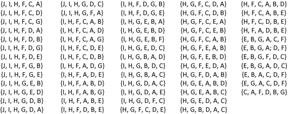
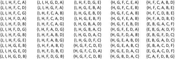
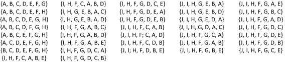
Set of minimal winning coalitions of the voting game v = (6; 1, 1, 1, 1, 1, 1, 1, 1, 1, 1) given Krackhardt’s kite network:
-
2.
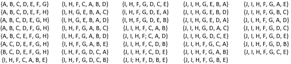
Set of minimal winning coalitions of the voting game v = (7; 1, 1, 1, 1, 1, 1, 1, 1, 1, 1), representing a 2/3 quorum, given Krackhardt’s kite network:
-
3.
Set of minimal winning coalitions of the voting game v = (6; 1, 1, 1, 1, 1, 1, 1, 1, 1, 1), given the D-modified Krackhardt’s kite network:
-
4.
Set of minimal winning coalitions of the voting game v = (7; 1, 1, 1, 1, 1, 1, 1, 1, 1, 1), representing a 2/3 quorum, given the D-modifiedKrackhardt’s kite network:


Rights and permissions
Copyright information
© 2019 Springer-Verlag GmbH Germany, part of Springer Nature
About this chapter

Cite this chapter
Holler, M.J., Rupp, F. (2019). Power in Networks: A PGI Analysis of Krackhardt’s Kite Network. In: Nguyen, N., Kowalczyk, R., Mercik, J., Motylska-Kuźma, A. (eds) Transactions on Computational Collective Intelligence XXXIV. Lecture Notes in Computer Science(), vol 11890. Springer, Berlin, Heidelberg. https://doi.org/10.1007/978-3-662-60555-4_2
Download citation
DOI: https://doi.org/10.1007/978-3-662-60555-4_2
Published:
Publisher Name: Springer, Berlin, Heidelberg
Print ISBN: 978-3-662-60554-7
Online ISBN: 978-3-662-60555-4
eBook Packages: Computer ScienceComputer Science (R0)