Markets for Liquid Fuels

Abstract

This chapter focuses on markets for crude oil and oil products including gasoline, kerosene, diesel, heating oil, as well as biogenic fuels such as biodiesel, bioethanol, and synthetic fuels. Since the mid-twentieth century, crude oil has been the world’s most important energy source. However, the future prospects of crude oil are more unclear than ever. A lot of issues have to be analyzed:

• What is the development of oil extraction?

• What technical and economic consequences are to be expected if conventional crude oil extraction falls short of the demand for liquid fuels?

• What about the so-called peak oil hypothesis from an economic perspective?

• At what oil prices would alternative fuels, such as unconventional oils, biogenic fuels, and liquefied coal become competitive?

• How can the structure of the oil industry be explained in economic terms?

• What is the role of governments in exporting and importing countries?

• What are the influences on the price of oil in the short, medium, and long term?

• What is the relationship between spot and future prices?

• To what extent are oil prices influenced by speculation?

This chapter focuses on markets for crude oil and oil products including gasoline, kerosene, diesel, heating oil, as well as biogenic fuels such as biodiesel, bioethanol, and synthetic fuels. Since the mid-twentieth century, crude oil has been the world’s most important energy source. However, the future prospects of crude oil are more unclear than ever. A lot of issues have to be analyzed:

• What is the development of oil extraction?

• What technical and economic consequences are to be expected if conventional crude oil extraction falls short of the demand for liquid fuels?

• What about the so-called peak oil hypothesis from an economic perspective?

• At what oil prices would alternative fuels, such as unconventional oils, biogenic fuels, and liquefied coal become competitive?

• How can the structure of the oil industry be explained in economic terms?

• What is the role of governments in exporting and importing countries?

• What are the influences on the price of oil in the short, medium, and long term?

• What is the relationship between spot and future prices?

• To what extent are oil prices influenced by speculation?

The variables used in this chapter are:

c :

Cost of carry (annualized cost of storage and insurance)

cy :

Convenience yield (advantage of holding the physical asset rather than a future contract)

dz :

Normally distributed stochastic variable

GDP :

Gross Domestic Product

i :

Risk-free interest rate

p :

Spot market price (indexed if it refers to a particular traded product)

p _F (T):

Price of a future with delivery date T

σ :

Standard deviation

Stock :

Stock of inventory

T :

Maturity (delivery date) in futures contracts

t :

Trading date

Vola :

Annualized volatility

8.1 Types of Liquid Fuels and Their Properties

Under normal atmospheric pressure, liquid energy sources are in a liquid physical state. This makes their storage, transferal, and transportation easy, i.e. low-cost. Furthermore, liquid energy sources have high energy density. For example, a 50 l gasoline tank has an energy content of about 32.4 ⋅ 50 = 1620 MJ or 450 kWh, respectively (see Table 8.7). Assuming that the filling of such a gasoline tank takes two minutes, the filling capacity of a gasoline pump amounts to 13.5 MW (= 30·450 kWh/h). A single gas station with eight gasoline pumps therefore has the potential to sell the same amount of energy (i.e. 108 MW) as 54 wind turbines with a capacity of 2 MW each. These advantages are the reason for the dominance of oil products in the transportation sector and their overall leading position in global energy markets since the mid-twentieth century.

However, reserves of crude oil are limited and likely to be exhausted in a not-too-distant future (see Sect. 8.1.3). Additionally, there is the environmental burden caused by the emission of greenhouse gases associated with the combustion of crude oil products. The content of the 50 l gasoline tank in the example above leads to the release of 117 kg CO₂ into the atmosphere. On a global scale, about 40% of energy-related CO₂ emissions derive from the combustion of crude oil. While these two issues represent important challenges in the foreseeable future, there is no general consensus about how to deal with them. For instance, it remains unclear whether renewable liquid fuels or renewable electricity will be able to substitute fossil liquid fuels to a sufficient degree.

8.1.1 Properties of Crude Oil

There are many data sources regarding crude oil, albeit in differing units of measurement. Therefore, the data need to be converted to a common energy unit. While there are conversion tables, they often fail to achieve comparability because crude oil is a natural product and thus a heterogeneous good. In particular, energy content differs between production sites, depending on the so-called crude oil density of the liquid. Thus, the conversion factors presented in Table 8.1 are based on a crude oil density of 0.858 kg/l or 7.33 bbl/ton, respectively.

Table 8.1 Standardized conversion factors for crude oil

For the oil industry, two crucial dimensions of quality are the density of hydrocarbon compounds and the viscosity of crude measured in API grades defined by the American Petroleum Institute (see Fig. 8.1). The economic value of crude increases with higher API grades. Therefore, condensates and light varieties fetch a higher price than heavy oil and tar sands. Crude oil varieties with values below 25° API count as unconventional oils. Below a level of 10° API, hydrocarbon compounds are not capable of flowing and hence transportation by pipeline. Another important characteristic of crude oils is their sulfur content. Low-sulfur oil is called sweet crude , whereas sulfur-rich oil is called sour crude .

Fig. 8.1

Properties of crude oil varieties. Sources: American Petroleum Institute; Erdmann and Zweifel (2008, p. 173)

American West Texas Intermediate (WTI) and European Brent are high-quality crudes serving as a benchmark, with around 42° API and sulfur contents below 0.3%. Other crudes such as Dubai Crude with 31° API and 2% sulfur content constitute the benchmark for oil from the Persian Gulf. Usually sulfur-rich oil is traded at a price discount compared to WTI and Brent (see Table 8.2). However, since these benchmark crudes are physically available at different locations, transportation bottlenecks and perturbations of local markets have resulted in price differences in excess of 25 USD/bbl in favor of WTI in recent years.

Table 8.2 Quality levels and prices of crude oil

8.1.2 Reserves and Extraction of Conventional Oil

Known and economically recoverable reserves of conventional crude oil are unevenly distributed over the globe. According to Table 8.3, more one-half of them are concentrated in the Middle East (most of it around the Persian Gulf) and in Central Asia. This region of the world plus Russia is known as the ‘energy ellipse’ which accounts for nearly 40% of global supply in terms of conventional crude oil.

Table 8.3 Reserves and extraction rates of crude oil, 2013

By way of contrast, the global share of crude oil extraction in OECD countries is far higher than their global share of reserves. Therefore, OECD countries will have less control over the supply of oil in future, while countries in the energy ellipse and OPEC (Organization of Oil Exporting Countries) countries can be expected to exert a growing influence on the global market for conventional oil. However, as expounded in Sect. 8.1.4 below, technological change has been increasing the supply of unconventional oil.

The effect if this geographic concentration is exacerbated by widely varying costs of extraction. While they are below 40 USD/bbl in the Persian Gulf on average, they can be as much as twice as high in other regions of the world (see Fig. 8.2). However, this cost advantage may be undermined by technological change . An example is the cost reduction in offshore production during the 1980s. In the early 1980s, retrieving oil from the North Sea cost 17 USD/bbl, causing production to become competitive only after the second oil price shock of 1979 when the sales price jumped from 10 to 30 USD/bbl. Yet, ten years later offshore production cost was down to 8 USD/bbl. This cost reduction occurred despite the fact that compared to other industries, the oil industry invests a small share of its earnings in research and development.

Fig. 8.2

Marginal cost of crude oil production (source: Oil Industry Trends)

8.1.3 Peak Oil Hypothesis

Motorization in the United States led to a phenomenal increase in oil consumption during the 1950s. It was during this decade that geologists began to address the question of how long it would take for crude oil reserves in the United States to be depleted. At that time, the U.S. share in global production exceeded 50%. In 1956, geologist Hubbert (1956, 1962) predicted that oil production in the United States would peak by 1970 and decline from then on (in the so-called lower 48 states, thus excluding production in Alaska and offshore drilling in the Gulf of Mexico).

His forecast proved true (see Fig. 8.3). It was based on a logistic function, which in the present context implies that the accumulation of production will approach an upper limit which equals total reserves (see Fig. 4.2). More specifically, according to the standard logistic function, rates of production begin to decline once one-half of total reserves have been retrieved (this is also known as the depletion midpoint ). By fitting observed production rates to the logistic function, Hubbert was able to determine the two parameters determining the logistic function, which in turn permits to predict the depletion midpoint and hence the year when the rate of production will attain its maximum.

Fig. 8.3

Crude oil extraction in the United States (source: EIA, CGES)

Note that the use of the logistic function can be justified with a change in marginal cost: At the start of exploitation, few oil fields are known and experience in exploration is lacking, causing the cost of locating an additional field to be high. With cumulated exploitation and production, the marginal cost of discovering and developing an oil field decreases, facilitating a high rate of production. Beyond some point however, marginal cost begins to increase again because easily accessible fields are depleted. This puts downward pressure on the rate of discovery and ultimately, the rate of production—unless the sales price of oil goes up in real terms, as e.g. during 1970s with its two oil price shocks (Kaufmann and Cleveland 2001; Reynolds 2002). Moreover, pressure in developed oil deposits declines with cumulated production. In order to compensate for this, water, steam, or carbon dioxide is pressed into the deposit, a process known as enhanced oil recovery . Of course, enhanced oil recovery is associated with an increase in the marginal cost of production; thus, it slows the decline in production rates but does not reverse the trend.

In the meantime, the peak oil hypothesis has been applied to global oil production on the grounds that global reserves are limited as well. In keeping with the Hotelling price path (see Sect. 6.2.2), lower-cost reserves are exploited first, followed by higher-cost alternatives such as Alaska in the case of the United States. Indeed, Fig. 8.3 exhibits rising, then falling rates of production. Yet, the figure also points to an intriguing constancy. In 1956, Hubbert predicted peak oil for 1970, i.e. 14 years away. In 1970, oil production in Alaska began to take off—and peaked again about 15 years later. Shortly after the year 2000, some experts saw the rate of global production peak 8 to 22 years into the future (averaging 15 years), while some others did not predict a peak at all.

The prediction of 8 years has already proved wrong since between 2002 and 2010, global production of crude increased in 8 out of 11 years at rates up to 5%, while the maximum decrease was −1.7%. Overall, it continued to increase up to 2013 (U.S. Energy Information Administration). Cumulated global oil production exceeded 1200 bn bbl in 2002; this is equivalent to 330 years of peak production in the United States (3400 mn bbl/a = 365·9.5 mn bbl/day as of 1970; see Fig. 8.3). Therefore, up to present economic incentives have been causing resources to be transformed into reserves at a pace that has kept up with growth in production and consumption. In hindsight, Hubbert’s success in predicting the 1970 peak in U.S. oil production, being based on the assumption of a predetermined amount of reserves, seems to be a coincidence rather than the result of in-depth analysis (Kaufmann and Cleveland 2001).

Table 8.4 shows estimates of the expected dates and the quantities of maximum conventional crude oil extraction, all of them published before 2004. In spite of differences which might be related to the affiliation of the respective experts, the consensus at the time was that depletion midpoint will be reached by 2020 or 2025 at the latest.

Table 8.4 Expert views on the production maximum of crude oil

Indeed, economists including Adelman (2002) and Lynch (2002) have argued that it has been possible to overcome resource scarcities through innovation up to now, suggesting that this might hold true in future as well. For example, Fig. 8.3 shows that the production decline in the United States predicted by Hubbert was substantially delayed thanks to advanced extraction technologies and the development of new oil fields (Alaska, deep offshore). At present, this view is confirmed by the growth of oil production in North America and other regions. Specifically, the ‘cracking revolution’ has again made the United States one of the largest oil producers worldwide and may even transform it into a net oil exporter before long. Globally, there are many inventions that have the potential to result in innovative technologies that will delay the peak in oil production (see Sect. 8.3.2, Fig. 8.10).

Sometimes the peak oil hypothesis is claimed to be supported by the fact that several private oil companies had to adjust their crude oil reserves downwards in recent years. But their reporting of reserves does not only depend on geological facts but also on institutions governing the market (see Sect. 6.1). Today, many oil fields are exploited under so-called production sharing agreements between public (governmental) and private partners. The private partner obtains a share of the reserves designed to ensure a rate of production and hence sales revenue that is sufficient to cover the cost of extraction plus a negotiated return on invested capital, while the public partner retains the rest. In case of rising oil prices, production sharing agreements typically permit governments to reduce the private share of reserves on the grounds that the same sales revenue can now be obtained from a lower rate of production (which is true in view of a short-term price elasticity of demand below one, as evidenced in Table 5.3. This causes the private partner to report less reserves, even though one would expect that rising oil prices lead to an increase in reserves.

8.1.4 Unconventional Oil

Unconventional crude oil includes heavy crude oil , oil sands , bitumen, tar sands, and shale oil . While estimates of reserves vary, the existence of huge deposits of heavy oil and tar sands is not in doubt. Deposits in the Orinoco basin in Venezuela and sands in Western Canada alone amount to 300 bn bbl of oil, a substantial addition to global reserves of conventional oil of roughly 1200 bn bbl (see Table 8.3).

Thanks to technological change, unconventional reserves can sooner or later be retrieved at a cost that makes them competitive against conventional alternatives. Oil sands even enjoy an advantage over conventional crude because their deposits are already known, obviating most expenses for exploration. However, extracting unconventional oil is far more complex and hence costly than extracting conventional crude. For this, there are two commonly used processes with the following properties:

• In the case of surface mining, oil sands are dredged and mixed with hot water. This mixture, also called slurry , is pumped through pipelines to treatment plants, where the bitumen is separated from the sand, mineral clay, salt, and water. After cleaning, the sand is recycled to fill the excavated mine, while the water is channeled to sedimentation tanks, to be used again eventually.

• In the in situ process, hot steam or CO₂ is injected into the oil layer in order to dilute the bitumen and make it flow. This mixture is extracted using conventional crude oil production technologies (i.e. steam-assisted gravity drainage, vapor extraction, and cyclic steam simulation). The in situ process also allows extraction of unconventional oil from deep deposits. A more recent technology is fracking , which was first applied to shale gas (see Sect. 9.1.2) but is now also used to retrieve shale oil.

As a rule, the production of unconventional oil is more expensive than the extraction of conventional crude oil. It also causes a greater environmental burden in terms of land use, energy input, and risks to drinking water. However, hikes in the price of crude oil have triggered large inflows of capital into research and development of extraction technologies as well as the development of unconventional deposits, preparing the ground for future growth of production.

8.1.5 Refineries and Oil Products

Profit margins are significantly higher in the extraction than in the refinery business, but refineries still represent the technological core of the oil value chain. In refineries, crude oil is processed into final energy sources such as gasoline, kerosene, diesel, and fuel oil. Their properties are listed in Table 8.5.

Table 8.5 Properties of crude oil and oil products

The refinery process can be divided into several sub-processes. Traditionally, the most important sub-process is distillation , where the chemical components of crude oil are separated in so-called fractions through heating and evaporation. Having different boiling temperatures (with water highest at 100 °C), they can be made to condensate at different levels in distillation towers. Particularly light fractions like methane, ethane, propane, and butane are collected at the top of the tower as so-called condensates or refinery gas . They are followed by gasoline and diesel in the medium levels, and residues in the lower levels of the tower.

Evidently, only products that are part of the raw material can be obtained through distillation. Yet refinery operators aim to maximize the output of light oil products which can be sold at higher prices. To increase their share, heavy fuel oil and distillation residues are further processed in conversion plants where their long and heavy hydrocarbon molecules are split into shorter and lighter molecular chains using so-called cracking.

There are three types of cracking processes: thermal, catalytic, and hydro cracking. In thermal cracking, the molecular bonds of large hydrocarbon molecules are broken up by heating the distillation residue up to a temperature of about 500 °C. Catalytic cracking uses a catalyst, e.g. synthetic aluminum silicate, for breaking up molecular bonds. The most flexible but also most costly conversion technology is hydro cracking . Here, hydrogen atoms are added at the ends of broken molecular chains in order to chemically stabilize them, making it possible to mainly produce gasoline and diesel. However, the process requires operation under high pressure (100–150 bar) and large quantities of hydrogen , often calling for the construction of a hydrogen-producing plant.

Table 8.6 shows a typical product portfolio of modern refineries. Without conversion, no more than 22% of output is gasoline, while up to 60% is lower-valued heavy oil. Catalytic cracking increases the gasoline share to 47%, hydro cracking, even to a maximum of 55%.

Table 8.6 Product portfolio of modern oil refineries

Refineries reach an average efficiency of about 82%. This is a high value since transportation to filling stations and other customers is deducted from output. Thus, the energy contained in all refined products sold to final consumers amounts to a 82% of total energy input from crude oil, natural gas, electricity, diesel, and gasoline.

An important managerial decision is where to locate a refinery. A distinction can be made between supply-oriented locations close to extraction sites and sea ports in importing countries and sales-oriented locations close to final consumers. Both types come with advantages and downsides. Sales-oriented locations facilitate cost-efficient, high-volume transportation of crude by pipeline and supertanker. This enables refineries to quickly adapt to changes in the structure of demand. Conversely, supply-oriented locations of refineries require more complex logistics because different products need to be transported over long distances. However, when sales prices are volatile and differ between destinations, supply-oriented locations make arbitrage possible. Oil companies simply redirect their deliveries (often already en route on the open sea) to the destination with the highest sales price (which usually offers the highest profit margin in view of low extra transportation cost). Therefore, supply-oriented locations of refineries may increase company profits while contributing to a convergence of prices of refined products.

8.1.6 Biogenic Liquid Fuels

Whereas in most uses of energy, oil products are in competition with other fossil fuels such as natural gas and coal, they continue to dominate in the transportation sector. Electric railways aside, this sector depends almost exclusively on oil. Yet considerable effort is being undertaken to introduce alternative fuels for transportation. The motivation is not only to enhance the security of energy supply by lessening the dominance of oil but also to reduce greenhouse gas emissions. Since these emissions are substantial in the conversion of gas to liquid (GtL) and coal to liquid (CtL), respectively, use of biomass as a liquid transportation fuel has been gaining attention. There are several options for biomass to liquid (BtL):

• Biodiesel (rapeseed oil methyl ester ) is produced from oily plants (e.g. rape, soy, sun flower). Oil gained from conventional oil mills (e.g. rapeseed oil) contains viscous components (see Table 8.7) and therefore needs to be converted into fatty acid methyl ester (FAME) in order to become a diesel substitute. Furthermore, methanol is added to make up about 10% of the final product, which can be marketed as pure biodiesel or added to conventional diesel (so-called blending ). In the European Union biodiesel production reached a volume of 9 mn tons by 2010 but has been declining since because biodiesel offers only limited environmental advantages over diesel. Its production cost varies between 0.55 and 0.70 EUR/l diesel equivalent. Assuming equal tax treatment of diesel and biodiesel, the renewable fuel would be competitive at prices of crude in excess of 100 USD/bbl only.¹

• Bioethanol (alcohol ) is produced by the fermentation of plants with high sugar content. In 2014, worldwide bioethanol production has reached 90 bn liter (of which the United States accounts for 57% and Brazil for 27%). Bioethanol is mostly sold as blend (as E10 in parts of the European Union, which is 90% gasoline and 10% bioethanol) because this obviates adjustments in refueling infrastructure and gasoline engines. Production cost of bioethanol ranges from 0.20 USD/l in Brazil to 0.35 USD/l in the United States and on to 0.55 USD/l in the European Union. The energy equivalent of one liter of bioethanol corresponds to 0.65 liter of gasoline. This makes Brazilian bioethanol competitive at prices of crude oil of 50 USD/bbl while European ethanol becomes competitive at prices above 140 USD/bbl only.

• Biofuels of the second generation (also known as BtL, biomass to liquid ) are produced using advanced technologies such as biomass gasification with a subsequent Fischer-Tropsch synthesis. Another innovation in the making is the utilization of enzymes for decomposing fibrous parts of plants designed to allow the energetic use of the entire plant mass. Unfortunately none of these technologies have been proven to be feasible outside the laboratory up to now.

Table 8.7 Properties of liquid fuels

With the exception of Brazilian ethanol, the supply of biofuels at present depends on political support such as (partial) exemptions from fuel tax and mandatory blending quotas for gasoline and diesel. Additionally, there are agricultural subsidies. The subsidization of biofuels has been justified by arguments derived from the theory of innovation. By creating a market niche for the corresponding technologies and cultivation practices, an industry can benefit from learning effects which might lead to cost reductions. The hope is that in future, increasing market shares can be obtained without political support (see IEA 2000; Nakicenovic 2002). The risk is that this support creates a pressure group that has a strong interest in its continuation. Experience shows that subsidies in particular are very difficult to terminate.

The production of biofuels is limited by the availability of arable land and yields. It can have a potentially negative impact on food security but also on biogas production (see Sect. 9.1.3). Table 8.8 shows the present range of yields for grains and oil plants in Central Europe. Using the example of biodiesel, 3.3 tons of rapeseed can be harvested per hectare given medium yields, resulting in 1.3 tons of rapeseed oil (given a yield of 0.4 tons rapeseed oil per ton rapeseed). Using the heating value of 37.6 MJ/kg in Table 8.7, the energy content of this harvest can be estimated at 49,000 GJ. About one-third of this energy is needed as an input into its transformation into biodiesel, leaving some 33,000 GJ per hectare for energy use. According to Table 8.7, this is the energy content of 1000 l biodiesel (32.6 MJ/l∙1000 l ≈ 33,000 GJ) or 900 l diesel equivalent.

Table 8.8 Yields of energy plants

These yields could be increased in the future through the use of seeds that are especially developed for the production of energy plants. Some agricultural experts believe that a 50% increase of yield is achievable.

Some years ago, the European Union aimed to increase the share of renewable energies in the transportation sector to 10% by 2020 (directive 2009/28/EG). This would require an agricultural area of more than 15 mn ha, or about 10% of the arable area in the European Union. In the meantime however, EU strategy has changed in favor of electric vehicles.

8.2 Crude Oil Market

During the 150 years of its history, the oil industry has gone through clearly distinct phases, which were characterized by differing market structures. Transition between these phases caused major changes affecting the oil industry, market participants, and the governments of oil-producing and oil-importing countries. It is important to understand the reasons for the relative stability during these phases as well as the transitions between them. This calls for the application of economic theory, in particular industrial economics and game theory.

8.2.1 Vertically Integrated Monopoly

Oil production on an industrial scale began in 1859 in Pennsylvania (United States). With the development of distillation technology, kerosene produced from crude oil became the preferred energy source for lighting. Previously, oil lamps had been fueled with whale oil, almost causing the extinction of whales due to overfishing. Thus, the substitution of whale oil by crude oil can be cited as the timely solution to an urgent resource problem.

Thanks to its advanced refining technology as well as rude competitive practices, the Standard Oil Company founded by John D. Rockefeller was able to achieve a monopolistic position on the American refinery market within a decade. After 1880, the company became a dominant player also in the U.S. extraction, transportation, and distribution business. However, pursuant the Sherman Act of 1890 (also known as Antitrust Act ), in 1911 the Standard Oil Company was split into 34 independent companies. Over time, some of these companies (Amoco, Chevron, Conoco, Exxon, Marathon, and Mobil) developed into the so-called oil majors that continue to operate on a worldwide scale to this very day.

The typical feature of oil majors is their vertical integration , meaning that they control the value chain from prospection, extraction, and transportation on to distribution to final consumers. What was the reason that the new oil industry evolved rather quickly into a vertically integrated monopoly (up to 1911)? The answer derives from an economic analysis of vertical integration, which emphasizes its efficiency advantages. Traditionally, economists have associated efficiency with arms-length market transactions, which are replaced by in-house command-and-control relationships in vertically integrated companies. Yet according to Grossman and Hart (1986), command and control tends to lose any initial efficiency advantage because the corrective of market competition is absent.² They argue that vertically integrated companies survive and may even dominate markets because they are able to force competitors out while preventing market entry by potential newcomers. Indeed, the oil industry’s value chain has several characteristics that facilitate dominance by a vertically integrated company:

• Kerosene and other oil products are commodities with relatively homogenous properties. In this situation, the famous law of one price holds. Thus, a refinery operator who has lower cost of production than its competitors (e.g. thanks to better equipment) has a competitive advantage. If in addition the refinery stage exhibits economies of scale (i.e. marginal cost and with it, average cost declines with increasing volume of output), the company with the initial cost advantage can achieve an ever growing market share, leaving no chance to smaller competitors and newcomers.

• A company dominating one stage of the value chain may be able to extend its control to the next stage, e.g. by creating a network of sales outlets that closes the market to independent retailers (so-called vertical foreclosure , see Tirole 1988, p. 193). In the case of Standard Oil, vertical foreclosure was first achieved ‘upstream’, by making railway companies depend on its high volume of orders for transporting crude oil and finally buying them up. In this way, competing refineries were cut off from the supply of crude oil. In a second step, Standard Oil also performed ‘downstream’ foreclosure by so-called exclusive dealing, i.e. by creating a dense network of gas stations that agreed to purchase their supply from Standard Oil only.

However, vertical integration has also been viewed in a more favorable light, starting with the work of Nobel laureate Coase (1937) who was first to highlight the role of transaction costs . Transaction costs comprise the collection of information e.g. on the quality of the product or service to be traded, setting up contracts, and monitoring compliance with them. In the presence of low transaction costs, arms-length dealing through markets is efficient. Yet when transaction costs are substantial, performing transactions within a company rather than through markets may be more efficient. A famous example is putting together a team for producing a movie. The market solution would require every actor, every costume designer, and every grip to strike a contract with every other member of the team. The internal solution is for the director to be partner to all contracts, giving him a measure of command-and-control authority. Note that as long as vertically integrated companies remain in competition with each other, vertical integration is subject to the market test so may well be beneficial at both the microeconomic and the macroeconomic level. In the case of refining companies, there are at least two reasons for efficiency-driven vertical integration:

• According to Williamson (1971), investments in refineries are asset-specific (also known as factor-specific investments ), meaning that they cannot be used for anything else but processing crude oil. In addition, refineries crucially depend on a continuous supply of crude oil, making them vulnerable to a ‘hold-up’ by oil extractors. Conversely, extracting companies would suffer from a ‘hold-up’ by refineries as soon as they rely on pipelines for low-cost transportation. In this situation, vertical integration can be an efficient alternative because it reduces the supply risks confronting refineries while stabilizing sales and earnings at the extracting stage. This makes investment in a vertically integrated industry attractive.

• Asymmetry of information between buyer and seller can be a problem calling for vertical integration. Usually, the seller knows more about the properties of the product than the buyer, who may have to undertake costly search for information. The buyer can avoid this cost by acquiring the seller, thus obtaining the right to inspect the product. During the early phase of the oil industry, asymmetric information was indeed a problem: The owner of an oil field had detailed knowledge about the quantity of oil in the ground, which the refinery operator lacked, being an outsider. However, a potential investor needed to have a reliable estimate of future supply in order to plan the refinery’s capacity. The purchase of the oil field resolved this asymmetry of information.

If highly asset-specific investment combines with risk in market transactions along the value chain, a tendency towards vertical integration is to be expected. However, this tendency hurts the economy in case it leads to ‘downstream’ monopolization to the detriment of final consumers. For small countries, it may be sufficient to keep markets open to foreign competition, exposing domestic producers to the threat of market entry by newcomers from the world market. However, these newcomers may be multinationals who have at least as much market power as their domestic competitors, calling for intervention by competition policy (Zweifel and Zäch 2003). In large countries like the United States, the world market may be dominated by its own domestic producers, creating a situation that cannot be resolved without government regulation designed to prevent the abuse of market power. In the case of the Standard Oil Company, application of the Sherman Act of 1890 (known as the Antitrust Act ) led to an extremely severe intervention, i.e. the forced unbundling of the monopolist. While vertical integration continues to characterize the oil industry, a vertically integrated monopoly is no more possible.

8.2.2 Global Oligopoly of Vertically Integrated Majors

With the shift from kerosene lamps to electric light, the market initially targeted by refineries vanished. Yet by historical coincidence, the combustion engine (with the gasoline engine patented in 1876 and the diesel engine, in 1892) created a new and much larger market for crude oil and its products. However, motor cars consume substantially more energy than kerosene lamps, causing people to worry already at that time whether there would be sufficient crude oil in the face of mass motorization.³ With the discovery of large oil fields in Texas (in 1901) and in the Persian Gulf region (Iraq in 1904, Iran in 1908, and Saudi Arabia in 1921), these concerns vanished.

As a consequence of this shift of supply to the Persian Gulf, the successors of the former Standard Oil Company had to expand their sourcing of crude oil in order to hold on to their market position. Internationally, they were competing with European companies such as BP and Royal Dutch/Shell, who had started their oil business in the colonies of their home countries. This globalization had the added benefit of permitting to shift profits within the vertically integrated organization towards tax jurisdictions offering favorable terms. In this context, internal transfer prices (also known as posted prices ) can be used to e.g. overcharge services provided by headquarters to an extracting division operating in the Persian Gulf. This leads to a reduction of profits recorded there, resulting in a lowered overall tax burden, provided the home country (which can be a tax haven like the Bahamas) offers a lenient taxation of profits.

By the 1920s, exploration of oil fields in the Persian Gulf exceeded growth in oil demand, leading to a fall in both the nominal and real price of crude (see Fig. 8.4). The U.S. Sherman Act of 1890 had created a new competitive environment which prevented the leading companies from individually controlling the market. In the aim of stopping the decline in oil prices, the three companies BP, Shell, and Exxon signed the Achnacarry Agreement in 1928, to be joined by Mobil, Gulf, Texaco, and Chevron later. This agreement froze the market shares of participating companies in all countries except the United States. A company who attracted additional customers was to share the extra demand with its competitors. Inevitably, the Achnacarry Agreement also froze market shares in the supply of crude. It constitutes a classic cartel designed to fix sales and production quotas. Also called the ‘seven sisters’ because it comprised the seven oil majors, it was able to control the international oil market until the 1970s. In particular, it thwarted attempts by the governments of concession countries to appropriate a greater share of profits by threatening to move production somewhere else. It also staved off nationalization, the most famous example being the creation of the National Iranian Oil Company in 1951 by Prime Minster Mosaddegh, who was ousted by a coup d’état led by British and U.S. intelligence agencies in 1953. From the viewpoint of the oil majors, their cartel was quite successful in keeping concession fees at a low level.

Fig. 8.4

Crude oil prices between 1900 and 2013 (data source: BP)

At that time, there was no antitrust legislation in most countries, with the exception of the United States. Indeed, for strategic reasons the U.S. government even encouraged domestic oil companies to expand worldwide. It saw no reason to intervene against the cartel because the Achnacarry Agreement explicitly exempted the United States, thus complying with U.S. antitrust legislation. Governments of the remaining consumer countries had no incentive to intervene either, likely because they viewed ‘their’ company as a conduit for transferring profits and hence tax revenue from producing countries. In fact, they benefited from a high import price, having started to tax gasoline in terms of a percentage levied on it.

Economists maintain that no cartel can live forever without an effective enforcement mechanism (often the government) because each of its members has an incentive to chisel. The temptation to sell more by secretly granting a price reduction is strong because the agreed sales price is usually way above marginal cost. Yet in the case of the ‘seven sisters’, the challenge came from another cartel, the Organization of Oil Exporting Countries (OPEC). This cartel became possible because governments of producer countries had achieved an increased degree of control over extraction (see Sect. 8.2.3).

In the wake of oil field nationalizations after the Second World War, the amount of crude available to oil majors fell short of their refinery capacities (see Fig. 8.5). As a consequence, these companies had to purchase crude oil on the international market to keep their refineries running. This made high prices of crude oil a mixed blessing for them: On the one hand, they reaped windfall profits on production from the fields remaining under their control; on the other hand, they incurred increased costs for purchasing the extra crude. In addition, the companies found it increasingly difficult to obtain new concessions in countries with nationalized oil fields. While there were alternatives such as domestic offshore oil and enhanced oil recovery (mainly shale oil at present), they continued to be more costly than production in Persian Gulf region. A further challenge was that some oil-producing countries began to process crude oil on their own. This led to global refining overcapacities and decreasing refinery margins (see Sect. 8.1.5).

Fig. 8.5

Extraction and refinery capacities of oil companies. Data source: www.energyintel.com

As a reaction to these challenges, private oil companies went through a wave of mega mergers by the end of the 1990s (see Table 8.9). As their motivation, they stated cost reductions and synergy effects, especially through an integrated optimization of refineries, logistics, and stocks. However, these mergers allowed the oil majors also to better control production capacities and oil flows, serving to boost their refinery margins and hence profits.

Table 8.9 Mega mergers between oil majors

8.2.3 The OPEC Cartel of Oil-Exporting Countries

In September 1960, five countries (Iran, Iraq, Kuwait, Saudi Arabia, and Venezuela) founded OPEC, the Organization of Petrol Exporting Countries. Its objective was to forge a joint monopoly that could set a sales price in excess of the competitive market price. However, a high price entails a reduced quantity sold; therefore, a cartel must allocate production quotas to its members. Yet in view of high profit margins, each member has an incentive to chisel, i.e. to secretly sell additional amounts at a reduced price, thus undermining the cartel.

Over time, more countries joined OPEC: Qatar (1961), Indonesia⁴ (1962), Libya (1962), the United Arab Emirates (1967), Algeria (1969), Nigeria (1971), Ecuador⁵ (1973 and 2007), Gabon (1975) and Angola (2007). While these additions caused the market share of OPEC to increase during the 1960s (see Fig. 8.6), the member states were not able to capitalize on this development. This changed in 1970 when Libya and Algeria, two relatively small oil-producing countries, were able to negotiate higher concession fees with ‘their’ private oil companies. They were successful for two reasons. First, the increase amounted to only 0.40 USD/bbl; second, the companies operating in these countries were not oil majors but relatively small companies without alternative production sites. The success of these two small OPEC member states shed a negative light on larger OPEC countries as well as on OPEC as a whole, who had obviously failed to take advantage of the cartel’s potential. However, OPEC soon had the opportunity to rectify this.

• The Yom Kippur War between Israel and its Arab neighbors in the fall of 1973 had a rallying effect on OPEC countries, who agreed to unilaterally increase the concession fee (in the guise of the so-called posted price ⁶) by a factor of five, to 11.65 USD/bbl. This hike has become known as the first oil price shock. The oil majors were not able to shift their business elsewhere (North Sea, Alaska) in the short term. Therefore, OPEC did not lose market share until about 1977 (see Fig. 8.6).

• The second oil price shock occurred in 1979, as a consequence of the Iranian Revolution (also known as Islamic Revolution ). With Saudi Arabia already having cut oil production by 25%, the political turmoil in Iran exacerbated the shortage, pushing the crude oil price from about 10 USD/bbl to over 30 USD/bbl. This time OPEC lost one-half of its market share because the oil companies were better prepared to shift their sourcing away from the Persian Gulf, to the North Sea in particular. In early 1986, Saudi Arabia (who had been stabilizing the cartel by accepting falls in its quota) decided to defend its market share by letting price drop to below 20 USD/bbl (see Fig. 8.6). This caused the OPEC cartel to break apart.

Fig. 8.6

Crude oil price and OPEC market share (data source: BP)

The two oil price shocks constitute the most important events of the twentieth century affecting the energy economy. They reflect the effectiveness of the OPEC cartel , who at least temporarily had acquired control over the global market for crude oil. Starting in 1982, OPEC countries had set extraction quotas that were compatible with a target price. Saudi Arabia, the OPEC country with the largest oil production by far, took on the role of the so-called swing producer by adjusting its production to achieve the desired price when other cartel members exceeded their quota. Between 1986 and 1999, however, Saudi Arabia was no longer willing to accept chiseling. In 1999 the quota system was reactivated in modified form. Semi-annual negotiated adjustments were replaced by an automatic adjustment if price (based on a basket of crudes sold by OPEC countries, the so-called OPEC basket ) deviated from a defined range. This system has never come under pressure since 2004 because oil prices have been exceeding this range as OPEC countries lacked the capacities to meet the growing demand for oil in Asia, in particular China (see Fig. 8.6).

To conclude, OPEC has been able to influence and at times even control the global oil market. However, it has repeatedly experienced periods of weakness. As with all cartels, its members have an incentive to violate the cartel agreement by selling more than their quota (at the high price secured by the cartel), unless there is an effective sanctioning mechanism. This lack of cooperation can be explained by a game theoretic model, the so-called prisoner’s dilemma (this term reflects the fact that two accomplices would have to be dismissed for lack of evidence if they cooperated; yet each one has an incentive to tell on the other, striking a deal with police).

Table 8.10 contains an illustrative example. For simplicity, OPEC is divided into two groups (Saudi Arabia and the rest of OPEC), each extracting 10 mn bbl/day. If both parties cooperate, the cartel can achieve a price of 60 USD/bbl; if they fail to cooperate, the competitive price of 40 USD/bbl obtains. However, there is another possibility: One party cooperates by sticking to its quota, while the other party chisels by selling in excess of its quota at a lowered price. Assume that each party is able to take over 50% of the other party’s demand if it lowers the price by 10 USD/bbl to 50 USD/bbl. Then, its revenue equals 750 mn (= 50·15) USD/day, whereas the cooperating party has revenues of only 300 mn (= 60·5) USD/day.

Table 8.10 Payoff matrix for OPEC members in mn USD/day (example)

The so-called payoff matrix shows the revenues accruing to Saudi Arabia and the rest of OPEC for the four combinations of strategies (see Table 8.10). Evidently, with 1200 mn (= 60·10 + 60·10) USD/day, cooperation maximizes the joint payoff, while failure to cooperate minimizes it (800 mn = 40·10 + 40·10). However, non-cooperation is profitable if the other party continues to cooperate, i.e. to stick to its quota. Therefore, each member of the cartel has an incentive to chisel, undermining the stability of the cartel.

This example suggests that cartels are likely to be inherently unstable. ⁷ In the case of OPEC, cooperativeness is further challenged by the asymmetry characterizing its members. Countries with a small but wealthy population (e.g. Kuwait, Saudi Arabia, and the United Arab Emirates) are pitted against countries with a large and relatively poor population (e.g. Algeria, Iran, and Iraq). The governments of the second group typically rely on budgeted revenues from oil sales. This implies that they seek to sell more rather than less when the sales price drops (keeping ‘price × quantity’ constant), which results in a supply function with negative rather than positive slope. This puts high demands on cartel management by the first group, in particular Saudi Arabia (Griffin and Steele 1986, p. 141).

The two oil shocks had a major impact on the economies of oil-importing countries (see Hickman et al. 1987). On the initiative of Henry Kissinger, the U.S. Secretary of State at the time, the industrial countries of the western world established the Paris-based International Energy Agency (IEA) in 1974. One of its missions has been the creation of stocks sufficient to cover oil demand for 90 days, to be released in case of emergency following a joint decision by all IEA member governments.

Several governments have built up additional stocks of oil that are not part of the IEA crisis mechanism. One example is the U.S. Strategic Petroleum Reserve whose use can be decided upon independently of other governments. From an economic perspective, state-controlled oil stocks amount to compulsory national insurance against oil shocks. However, insurance coverage is known to induce so-called moral hazard. In the present context, it undermines preventive effort by private companies and consumers designed to deal with supply shortages. In fact, the amount of oil stocked by the private sector has significantly decreased with the introduction of state-owned stocks. Another problem is that governments may use oil stocks for other purposes than securing supply. In particular, some have released stocks in the past in order to reduce the price of oil products in an attempt to curry favor with voters at election time.

8.2.4 State-Owned Oil Companies

Nationalizations of private oil companies have a long history: Azerbaijan (1924), Mexico (1938), Romania (1948), Iran (1951-1953), Indonesia (1960), Algeria (1970), Libya (1971), Iraq (1972), Iran (1973), Venezuela (1975-1990), Canada (1975), Kuwait (1975), Saudi Arabia (1980), Venezuela (2004), Russia (2004), and Bolivia (2006) are just the most important cases.⁸ However, only two of the eight largest oil companies were state-owned in 1972. By 2000, the situation was reversed, with only two of the eight major companies being privately owned (ExxonMobil and Shell). The four so-called super majors (ExxonMobil, Shell, BP, and Total) account for no more than about 11% of global crude oil extraction. A new form of state control over crude oil markets thus originates in oil-consuming countries, whose state-owned companies have been more successful than the private oil majors in the acquisition of foreign oil concessions.

In most countries, oil deposits, as well as deposits of other raw materials, are owned by the public sector, most often by central government. This also applies to offshore fields within the 200-mile economic zone. The transfer of extraction rights to private companies is based on extraction licenses or so-called concessions. In principle, governments are free to decide whom to award these licenses except that they have to respect international agreements, for example OECD norms regarding foreign direct investment or non-discrimination norms of the European Union.

Whether the extraction of raw materials, notably crude oil, should be allocated to the private or the public sector has been hotly disputed since the nineteenth century. Yet there is an economic argument in favor of oil extraction by public companies, derived from so-called principal-agent theory . This theory revolves around a principal who hires a specialized agent whose effort it cannot observe, a situation which creates leeway for the agent to pursue its own interest. To a government acting as the principal, effort deployed and cost incurred by a private company (the agent) are indeed largely unobservable. Thus governments are exposed to the risk of opportunistic behavior on the part of e.g. private oil companies, a risk that cannot be entirely eliminated even by contracts of the most sophisticated type. Therefore it may be preferable for governments to directly control oil production through their own national oil company (whose effort is assumed to be open to inspection).

Rosa (1993) has elaborated this argument further. His starting point is that “(…) the rationale for nationalization is to be found in the basic business of politics, the transfer motive” (Rosa 1993, p. 320). In order to appropriate the maximum amount of money from the oil industry, governments can tax extraction profits or nationalize the oil extraction business.⁹ Either way, they obtain most of the scarcity rent associated with an exhaustible resource (see Sect. 6.2.1). Their rational choice depends on the cost-benefit ratio of these two alternatives. Since these cost-benefit ratios vary over time, the optimal choice may also vary, which would explain the long historic waves of privatization and nationalization. In keeping with this line of thought, the propensity to nationalize oil extraction is predicted to increase if

• scarcity rents increase, since this favors opportunistic behavior by private companies. According to Fig. 8.7, the revenues from oil exports (which reflect profits to a considerable extent because costs were far more stable) correspond closely with the two waves of nationalization in the 1970s and after 2000;

  Fig. 8.7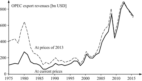

  

  OPEC revenues from oil exports (data source: EIA 2014)

• foreign oil companies act more aggressively to reduce their tax burden, causing income from profit taxation to fall;

• the degree of corruptibility of public officials increases, since this also tends to decrease income from profit taxation;

• the interest differential between private and public loans increases (given that it is positive) because interest payments by private oil companies lower their profits and hence tax payments while interest payments to former owners of nationalized resources become comparatively smaller;

• tax collection becomes more costly due to an increase in tax evasion and fraud.

Conversely, privatization becomes attractive if the government revenue generated by a national oil company falls short of the tax on profit attainable given that the company is privatized. Usually, this situation is the result of a high productivity gap between private and national oil companies. However, such a gap may in turn be caused by the fact that public companies pursue other goals than profit maximization (which goes along with high productivity). National oil companies may be used by government as a vehicle to reduce unemployment (through overstaffing) or to sell oil products to domestic consumers at below-market prices. Both measures correspond to the main business of government – transferring income and wealth to preferred voter groups (Hartley and Medlock 2008).

However, productivity gaps between private and public companies can be traced to other reasons, in particular a lack of innovativeness in state-owned firms. During periods of rapid innovation in the oil industry, the involvement of national oil companies in the extraction business tends to be harmful to the oil-producing country, motivating rational governments to privatize.¹⁰ Conversely, during periods of slow innovative change, governments are predicted to prefer state ownership.

8.3 Oil Price Formation

With the creation of national oil companies in the 1970s, the private oil majors ceased to be vertically integrated, with the inevitable consequence of a substantial expansion of international trade in oil. There are two types of traders on wholesale oil markets (see Fig. 8.5):

• Companies with a long position (net suppliers) who dispose of more crude oil than they can refine and therefore have an excess of crude oil. Typical examples are national oil companies, who lack not only refining capacities but also access to consumer markets since most filling station networks continue to be controlled by the oil majors.

• Companies with a short position (net demanders) who depend on crude oil purchases for utilizing their refining capacities and supplying their filling station networks. Typically, these are the oil majors, having lost many of their oil fields and extraction rights.

This structure encourages the development of wholesale oil markets. One has to distinguish between spot markets (for physical delivery), forward markets (ultimately for physical delivery), and markets for financial derivatives. On spot markets, conclusion of the contract, delivery, and payment occur more or less simultaneously. In the case of the oil industry, settlement is somewhat delayed for logistical reasons but usually does not take more than 15 days. On forward markets, delivery and payment are due several months or even years after conclusion of the contract. Volumes and prices are fixed ahead of delivery, permitting the party less able to bear risk to shift the risk (of a price change in particular) to the party who is better able to bear it, e.g. because its activities are more diversified (see Sect. 12.2.5 for an analogous discussion of forward electricity markets). On derivative markets, contracts relating to physical quantities rather than physical quantities themselves are traded, such as futures and options; accordingly, settlement is financial rather than physical. Derivative markets enable traders from outside the oil business, for example financial institutions, to participate.

Another distinction is between contracts concluded on an energy exchange or outside an exchange (so-called over-the-counter contracts, OTC for short). The reason for using energy exchanges instead of OTC markets is counterparty risk . Each party to a contract is exposed to the risk that the counterparty defaults, for instance due to insolvency. While this risk increases with time until settlement, it is eliminated if the energy exchange becomes the counterparty to the contract. The exchange is better able to bear this risk because it administers a huge number of contracts, causing the likelihood of multiple defaults to be very small. Still, exchanges acting as clearing houses protect themselves against financial risk by asking their members to provide collateral and to adjust it to market developments (so-called marking to market). This is the ‘price of the counterparty insurance’ and may amount to substantial transaction costs for traders. Another reason for using an energy exchange is anonymous trading; sellers and buyers do not need to know their counterparty.

The most important crude oil exchanges are the New York Mercantile Exchange (NYMEX) and the International Commodity Exchange (ICE) in London (formerly International Petroleum Exchange). Each defines a so-called benchmark crude for describing product quality. For the U.S. market this is West Texas Intermediate (WTI) traded at Cushing; for Europe it is North Sea Brent. More recently, Dubai Crude has been established as the benchmark crude for the Persian Gulf (see Sect. 8.1.1).

8.3.1 Oil Spot Markets and the Efficient Market Hypothesis

An important task of energy economists is to understand price developments on crude oil spot markets. According to the theory of efficient markets , the current spot price is the best possible forecast for the price of the following day (a so-called naïve forecast). The reason is that price incorporates all information available to market participants without any delay, causing daily spot prices p _t to follow a random walk . As there are no negative prices on the oil market, the logarithmic version of random Brownian motion is the appropriate model,

$$ \begin{array}{l} \ln {p}_t= \ln {p}_{t-1}+\mathit{\mathrm{Vola}}\cdot dz\;\mathrm{or}\\ {}\Delta \ln {p}_t= \ln {p}_t- \ln {p}_{t-1}= \ln \left(\frac{p_t}{p_{t-1}}\right)=\mathit{\mathrm{Vola}}\cdot dz.\end{array} $$

(8.1)

The stochastic variable dz ~ N(0, dt) is normally distributed, having expected value zero and variance dt, with dt denoting the time interval between quotations (e.g. a day if daily closing prices are to be analyzed). Vola symbolizes annualized volatility . It is calculated by multiplying the standard deviation σ of the logarithmic difference Δln p _t (the so-called price return ) by the square root of the 252 trading days per year (261 weekdays minus 9 public holidays),

$$ Vola=\frac{1}{T-1}\cdot \sqrt{{\displaystyle \sum_{t=1}^T{\left( \ln {p}_t- \ln \overline{p}\right)}^2}}\cdot \sqrt{252}=\sigma \cdot \sqrt{252}. $$

(8.2)

The original time series (ln p _t , t = 1, 2,…) with the property (8.1) has a stochastic trend. If the differentiated time series of price return Δln p _t is stationary and statistically white noise, ln p _t is said to be integrated of order one.

According to Fig. 8.8, the daily relative changes in the price of benchmark crudes can be approximated closely using the random walk model (8.1). For 420 days in 2005 and 2006, observed average volatility of WTI spot prices was equal to 0.020 ⋅ 252^0.5 = 32%. Kurtosis (reflecting the ‘thickness of the tails’) is 3.454, exceeding the value of 3 characterizing the normal distribution. This means that large relative day-to-day changes in price are more frequent than would be expected under a normal distribution [and hence the model (8.1)]. However, with 3.788 the Jarque-Bera test statistic (which amounts to a χ² with two degrees of freedom) indicates that the summed squared deviations from a normal distribution are too small to be statistically significant. More detailed analysis shows that Vola was not constant over time, contrary to the model (8.1), suggesting that the parameter estimates presented may not be robust to changes in the observation period. Yet, overall the hypothesis of efficient markets need not be rejected in the case of benchmark crudes.

Fig. 8.8

Histogram of Δln p _t for 420 days, 2005–2006

8.3.2 Long-Term Oil Price Forecasts and Scenarios

Naïve short-term price forecasts of the type presented in the preceding section are not satisfactory for an economic assessment of investments in the energy industry and for energy policy, which need to be based on long-term predictions. Accordingly, industry analysts (e.g. Prognoseforum in Germany), financial institutions (e.g. research divisions of commercial banks), research institutes (e.g. the Center for Global Energy Studies CGES), as well as public authorities (e.g. the International Energy Agency and the U.S. Department of Energy) regularly publish long-term oil price forecasts and scenarios.

Most commonly, they perform a so-called fundamental analysis , trying to predict future price developments by observing shifts in the supply of and demand for oil. Some factors influencing supply were mentioned in Sects. 6.2 and 8.2; at this point, a more comprehensive list of supply-side factors is presented.

• According to economic theory, the marginal cost of the last oil field needed to meet demand constitutes the lower bound of the price of crude oil. Over time, oil fields are exhausted, calling for the development of new fields which usually have higher marginal cost, however. Thus the marginal cost of crude oil tends to increase over time. In 2003, the Swiss Investment Bank CSFB estimated the break-even cost of crude oil extraction at 17.60 USD/bbl. Eleven years later, it was much higher (see Fig. 8.2). This partly explains the increase in the price of crude oil that has occurred since 2003. On the other hand, technological change can lead to a fall in marginal cost. This was particularly relevant in the 1980s and 1990s, contributing to a period of low oil prices (in real terms) between 1986 and 1999.

• Capacity utilization is another fundamental factor influencing price developments. When capacity utilization is low, an increase in the demand for oil can be met at little extra cost. In a market diagram, the supply schedule runs almost horizontal. When capacity utilization is high, extra demand can only be met by working overtime, working faster, and hiring more labor, all of which drives up marginal cost (in keeping with the adage, ‘haste makes waste’). The supply schedule has a steep slope, indicating that any increase in demand boosts price. On the longer run, capacity is adjusted, usually by bringing in new machinery that incorporates technological change and hence serves to lower marginal cost. The supply schedule shifts out, causing price to fall (provided demand does not continue to increase). The result is a cyclical development of the price of crude.

• Exploration and development of new oil fields may reinforce this cyclical pattern. The condition is that the new fields operate at the same or lower marginal cost as the existing ones, thus causing the supply schedule to shift out. Then, the cycle can be described as follows. At low capacity utilization and low demand, investment in new fields is unattractive (existing ones may even be abandoned). In this situation, a surge in demand causes the price of crude to rise. This triggers exploration effort, and with a lag of three to five years (Reynolds 2002), new discoveries result in an outward supply shift, which in turn exerts pressure on price.

• Available extraction capacities are not only influenced by economic considerations but also by wars, political boycotts, strikes, and expectations of such events. Political risks therefore have an impact on crude oil prices.

• Many analysts differentiate between capacity utilization in OPEC countries and in non-OPEC countries. In particular, large spare capacities in non-OPEC countries limit the potential of the OPEC cartel to increase oil prices. Conversely, spare capacities in OPEC countries can be irrelevant if cartel discipline of OPEC members is strong.

• More generally, the effectiveness of OPEC matters. It can vary greatly because the OPEC cartel is inherently unstable (see Sect. 8.2.3). Sometimes it can achieve a price markup over marginal cost, sometimes it cannot. Thus, analyzing the decision processes within OPEC, particularly during the bi-annual meetings of OPEC energy ministers, is part of fundamental analysis.

• In the case of an exhaustible resource, self-fulfilling expectations may induce volatility in price (see Sect. 6.2.3). If market participants expect increasing prices for crude oil, their production decisions differ from a situation in which they expect decreasing prices. Important sources for such expectations are scientific studies and their rendition in the media, in particular business newspapers. Arguably the first oil price shock caused by the oil boycott of OPEC in 1973 was amplified by the influential study by Meadows et al. (1972) on the limits to growth. Also, the oil price increase after 2000 coincided with a public debate about peak oil. In both cases, crude oil was believed to be in short supply before long, providing a seemingly sound justification for its price to increase.

• Prices of benchmark crudes are quoted at point of delivery. For WTI, this is Cushing, Oklahoma, for Brent it is the ports of Amsterdam, Rotterdam, and Antwerp. In the latter case, cargo rates directly influence price; rates in turn depend on availability of tanker capacity, fuel cost, and risk along major shipping routes (geopolitical for the Strait of Hormuz, piracy for the Strait of Malacca).

The most important demand-side factor for crude oil prices is growth of the global economy (see also Sect. 5.2). In order to empirically test this link, annual data on global economic growth rates published by the International Monetary Fund (IMF) can be used. A least-squares regression based on 24 observations covering the years 1990 to 2013 relates the relative changes in Brent spot prices p _Brent (data source: BP) and global GDP growth rates. The regression result reads

$$ \begin{array}{ccc}\hfill \frac{\Delta {p}_{Brent}}{p_{Brent}}=\hfill & \hfill -33\kern0.5em +\hfill & \hfill 12.5\cdot \frac{\Delta \mathrm{GDP}}{GDP}.\hfill \\ {}\hfill \hfill & \hfill \left(-2.97\right)\hfill & \hfill (4.20)\hfill \end{array} $$

(8.3)

The t-statistics in parentheses indicate statistical significance of the parameters, the coefficient of determination R² = 0.42 satisfactory statistical fit, and the Durbin-Watson statistic DW = 1.87, absence of serial correlation of residuals.

According to this estimation, global economic growth of 1% per year is associated with an increase in the Brent spot price increase of 12.5%, ceteris paribus. The ceteris paribus clause is important because market prices are determined by demand and supply, whereas Eq. (8.3) focuses on a demand-side influence only (for other influences, see below). Also, note that in the absence of growth (ΔGDP/GDP = 0), the equation predicts price to fall by 33%, likely due to the supply-side influences discussed above. Finally, ΔGDP/GDP should be viewed as endogenous, reflecting the fact that an increase in the price of oil hampers growth in most of the world economy, while a decrease fosters it. Reassuringly however, an estimate linking relative changes in WTI spot prices to global GDP growth from 1990 to 2005 yields comparable results, albeit with a more marked declining trend (Erdmann and Zweifel 2008, p. 202).

There are other factors on the demand side that may influence the price of crude oil:

• Quality requirements concerning oil products affect the structure of demand. Stricter environmental norms have served to increase demand for high-quality (sweet or low-sulfur, respectively) crudes relative to demand for low-quality (sour or high-sulfur) ones (see Sect. 8.1.1).

• For several oil-consuming countries, demand for internationally traded oil is a net quantity because they have domestic supplies. For instance, the development of fracking has been reducing demand for imported oil by the United States (the country is even predicted to become a net exporter before long). This puts pressure on the price of internationally traded crude.

Evidently, there is a multitude of factors influencing crude oil prices. Quite possibly, their relative importance is not constant over time, making fundamental analysis difficult. This also means that price forecasts derived from fundamental analysis are unlikely to be accurate. This consideration suggests scenario modeling as a more modest approach. Scenario modeling yields only conditional predictions reflecting varying assumptions concerning the future development of factors determining the price of oil.

Most of the published oil price scenarios are based on the concept of adaptive expectations ¹¹. Market participants are assumed to base their predictions on a linear combination of past prices and the currently observed price. By changing the relative weights entering this linear combination, analysts can generate price scenarios which amount to an extrapolation of trends estimated in different ways (see also Sect. 5.3.2). As an example, Fig. 8.9 exhibits oil price forecasts published by the U.S. Department of Energy (DOE). Forecasts are dashed lines showing future price paths predicted at the date of publication; actual price developments are represented by solid lines. As long as the existing price trend remains unchanged, these forecasts are relatively accurate. Yet whenever there is a change in trend, scenarios based on adaptive expectations can be seriously misleading.

Fig. 8.9

Crude oil price forecasts published by the U.S. Department of Energy

Changes in trend (also called structural breaks or regime shifts) occur only sporadically. They are attributed to factors that slowly reach or exceed a certain threshold value, when they suddenly become important. Non-linear systems theory has been the tool of choice for analyzing such regime shifts. An example of a ‘slow’ variable is the change in the relative cost of production of different technologies. Evidently, the condition for a regime shift is met if the cost of production using an alternative technology falls below the cost of the conventional alternative. However, this does not lead to massive investment in the new technology right away. In the case of fracking, factors causing delay were concerns about a future drop in the sales price of crude, environmental risks, and government intervention protecting incumbent players and technologies. Yet with a continuing or even increasing cost advantage of the new extraction technology, the regime shift cannot be halted.

The upper panel of Fig. 8.10 shows the succession of technologies in U.S. oil extraction since 1900. The first oil price shock of 1973 fostered investment in technology suitable for offshore extraction, the second of 1979/80, in technologies suitable for the retrieval of unconventional crudes, notably fracking. As argued above, the introduction of a new extraction technology causes a surge in supply which puts pressure on price for a few years. The lower panel of Fig. 8.10 displays the cascade-like development of price in a stylized way. It reflects the expectation that by 2035, biofuels and coal liquefaction may well cease a spike in oil price initially triggered by the exhaustion of unconventional sources of oil.

Fig. 8.10

Perspectives of crude oil supply. Source: Erdmann and Zweifel (2008, p. 207)

Figure 8.10 can also be related to the peak oil hypothesis which predicts that the sum of onshore and offshore oil extraction will reach its maximum soon (see Sect. 8.1.3). However, recurring price spikes have made the introduction of new extraction technologies profitable in the past, causing the maximum to shift forward. If crude oil supply should again fall short of demand in future, this shift is likely to be repeated, with biofuels, coal liquefaction (Coal to Liquids, CtL), and even more advanced technologies based on hydrogen electrolysis (Power-to-Liquids, PtL) taking over the role of shale oil.

8.3.3 Prices of Crude Oil Futures

Once liquid spot markets for benchmark crudes are established, markets for derivatives can develop. The most important derivatives are oil futures traded on energy exchanges. Futures are standardized contracts (1000 bbl of a benchmark crude) to be settled at standard delivery times (middle of the month) at a price agreed upon in advance. While settlement in terms of physical quantities is possible, financial settlement is more common. In this case, the difference between the spot price observed on the exercise day (the price of the so-called underlying) and the price of the future is paid. If the spot price exceeds the price agreed upon in the future, the buyer of the contract receives the price difference from the exchange while the seller has to pay this difference to the exchange. If the spot price is below the future price, the buyer of the contract has to make up for the difference while the seller receives it.

The standard example is the operator of a refinery with excess capacity. One alternative is to buy crude oil on the spot market and to keep it in storage for use months later. This strategy comes with the so-called cost of carry which comprises cost of storage and insurance as well as forgone interest on the capital tied up. Alternatively, the operator can buy a future contract with the appropriate maturity T. As long the two alternatives differ in terms of cost, there is scope for arbitrage which can be used by the refinery operator to reduce its cost of sourcing. Conversely, if no scope for arbitrage exists at trading date t, the market is in equilibrium, which implies the following relationship between spot price p _t and future price p _F,t (T) (Kaldor 1939; Hull 1999),

$$ {p}_{F,t}(T)=\kern0.5em {p}_t\cdot {e}^{\left(i+c\right)\left(T-t\right)}. $$

(8.4)

Thus, the price of the forward contract must equal the spot price accrued for interest i and cost of carry c during (T-t) time periods. Provided c is constant, Eq. (8.4) represents a cointegration equation of degree one, which means that the two time series, (p _F,t , t = 1,...) and (p _t , t = 1,...), cannot permanently diverge.¹² From Eq. (8.4), one therefore has

$$ \underset{t\to T}{ \lim }{p}_{F,t}(T)={p}_t $$

(8.5)

$$ {p}_{F,{t}_0}(T)>{p}_{F,{t}_1}(T)>{p}_t\kern0.37em for\;{t}_1>t $$

(8.6)

The no-arbitrage conditions predict four things. In view of Eq. (8.4), (i) the future price should increase over time as long as the spot price increases ceteris paribus; (ii) according to Eq. (8.5), the price of a forward contract with given maturity T should approach the spot price as time t goes on; (iii) the forward price should always exceed the spot price in view of inequality (8.6); and (iv) this excess should decrease over time since the difference (T-t) goes to zero, again in view of inequality (8.6).

Figure 8.11 displays so-called forward curves for contracts with a given maturity. The data confirm prediction (i) in that the forward curves shift up in response to increases in the spot price. They also confirm prediction (ii) until 2002 in that forward prices indeed approach spot prices as time goes on, causing t to approach T. The forward curves are said to be in contango during this period. However, more recently a tendency towards convergence cannot be observed anymore; the forward curves are said to be in backwardation . As to prediction (iii), it is not vindicated because the majority of forward curves runs consistently below the spot price. Moreover, given that they are above the spot price, the excess often fails to decrease as time goes on, contrary to prediction (iv).

Fig. 8.11

Oil forward curves between 1993 and 2006. Data source: Centre for Global energy Studies (CGES)

During periods of backwardation , futures with late maturity are cheaper than those with early maturity, indicating that the cost of holding a physical stock decreases rather than increases with time to maturity (T-t). The solution has been to complement Eq. (8.4) with a so-called convenience yield cy which may dominate the cost of carry c,

$$ {p}_{F,t}(T)=\kern0.5em {p}_t\cdot {e}^{\left(i+c-cy\right)\left(T-t\right)}. $$

(8.7)

The convenience yield could be due to the flexibility in use afforded by a stock of crude prior during time to maturity. While cy is constant in Eq. (8.7), Fig. 8.11 suggests it varies over time. Thus, this modification of the no-arbitrage condition (8.4) remains unsatisfactory as long as the convenience yield is not related to its determinants.

This challenge is taken up by the theory of normal backwardation (Hicks 1939, pp. 135–140), which explains the shape of the forward curve by a demand for hedging price risks which may differ between sellers and buyers and vary over time. In contango , buyers who seek to hedge their short positions dominate, while in backwardation, they are the sellers who want to hedge their long positions. The theory of backwardation is further explained in Sect. 12.2.5, where it is applied to the markets for electricity.

Another approach to explaining the development of price on the market for oil futures starts from the observation that the daily volume of derivatives traded (the so-called paper market) is 30–40 times bigger than the worldwide annual consumption of oil (the so-called wet market). This gives rise to the suspicion that in addition to fundamental market conditions, financial speculation might play a role.

For an analysis of speculative effects on price, backwardation and contango situations need to be considered separately. In the case of backwardation, speculators are predicted to purchase contracts with maturities far in the future (because they are cheap, see Fig. 8.11 again) while selling contracts with short-term maturities. As time goes on, contracts with long-term maturities become higher-valued contracts with short-term maturities. This strategy is profitable provided spot market prices do not fall (which would make a spot purchase an even better alternative). By way of contrast, in the case of contango arbitrage between short-term and long-term futures does not yield profits. The reason is that in contango it would be attractive to purchase contracts with short-term maturities before they become more expensive (see Fig. 8.11). However, as time goes on, these contracts cannot turn into higher-valued contracts with long-term maturity. The consequence of this behavior is that in backwardation, speculators buy up a lot of futures in the paper market, which serves to reduce quantities available on the wet market and hence to drive up spot prices. Conversely, in contango speculators stay away from the paper market, thus leaving supply to the wet market, which in turn causes spot prices to remain stable or even fall.

Indeed, between 2002 and 2006 (a period of backwardation), an inflow of financial capital into the derivative oil market amounting to at least 100 bn USD was reported by The Washington Post. This inflow may well have contributed to the increase in the spot price of crude from 30 to more than 60 USD/bbl in 2006. Likewise, the sudden outflow of financial capital in the autumn of 2008 may explain the drop to 40 USD/bbl in that same year.¹³

8.3.4 Wholesale Prices of Oil Products

As a first approximation, the wholesale price of an oil product is the sum of the crude oil price (i.e. the purchase price paid by refineries) and the cost plus margin of the refinery. In the literature, the spread margin is distinguished from the cash margin when quantifying refinery margins. The spread margin refers to the difference between the sales price of the oil product and the purchase price of the crude; it is transparent because it can be calculated from publicly accessible price data. The cash margin results from the difference between the revenue from selling the product and the cost of production. Its calculation requires knowledge of refineries’ cost of operation which is not available to outsiders.

In view of the range of refinery products and their prices, the calculation of the spread is also complicated, calling for simplifying assumptions. The following formula is often used for estimating the so-called crack spread of refineries,

$$ Crack\; Spread=\left(2\cdot {p}_{gasoline}+{p}_{fuel\kern0.5em oil}\right)/3-{p}_{crude}. $$

(8.8)

In keeping with U.S. market conditions, the price of gasoline is weighted double relative to the price of heating oil (which includes diesel). Since prices need to be per unit energy for aggregation, the price of gasoline p _gasoline , heating oil p _heatingoil , and crude oil p _crudeoil are converted to a common reference unit using their heating values (e.g. barrels of crude oil equivalent; see Table 8.1).

Figure 8.12 shows the crack spreads of U.S. and European refineries since 1993. Before 2000, the global refinery industry was characterized by large overcapacities (see Fig. 8.5). Once these overcapacities disappeared, the crack spread increased sharply. It is unlikely to return to its former levels since the refinery industry is heavily concentrated in most countries, facilitating collusion. In addition, barriers to entry are high for newcomers.

Fig. 8.12

Refinery margins (data source: BP 2014)

While crude oil prices and refinery margins do not display a seasonal pattern, there is one for refinery products, at least in the U.S. market. Summer is the driving season, during which gasoline prices are high relative to heating oil prices.¹⁴ Winter is the heating season, during which heating oil is expensive compared to gasoline. This pattern is confirmed by an ordinary least-squares regression based on weekly observations in the United States covering the years 2001 to 2014. The dependent variable is the ratio of prices for gasoline and heating oil; the explanatory variables are a seasonal term (represented by the cosine function), the available stocks of gasoline and heating oil, respectively, and a time trend that increases by one unit per week. The estimation result reads

$$ \begin{array}{cccc}\hfill \frac{p_{\mathit{\mathrm{Gasoline}},t}}{p_{\mathit{\mathrm{Diesel}},t}}=1.300+\hfill & \hfill 0.059\cdot \hfill & \hfill \cos \left(\frac{t-10}{8.3}\right)+\hfill & \hfill 0.00099\cdot {\mathit{\mathrm{Stock}}}_{\mathit{\mathrm{Diesel}},t}\hfill \\ {}\hfill (31.6)\hfill & \hfill (22.2)\hfill & \hfill \left(-26.0\right)\hfill & \hfill (8.1)\hfill \end{array} $$

(8.9)

$$ \begin{array}{cc}\hfill -0.0017\cdot {\mathit{\mathrm{Stock}}}_{\mathit{\mathrm{Gasoline}},t}\hfill & \hfill -0.0099\cdot \frac{t}{52}\hfill \\ {}\hfill \left(-7.6\right)\hfill & \hfill \left(-20.5\right)\hfill \end{array} $$

The t-statistics below the estimated parameters indicate that all coefficients are statistically significant, while the coefficient of determination R² = 0.62 indicates good statistical fit. However, the Durbin-Watson statistic DW = 0.08 points to a high degree of positive serial correlation between residuals. Therefore, when the predicted value of the price ratio exceeds the observed one for a given week, it is likely to be too high again in the following week. This lack of independence over time causes the standard errors of the coefficients to be underestimated and hence their t-statistics to be overestimated. It often reflects a neglect of additional explanatory variables, which in turn may result in biased parameter estimates.

With these reservations in mind, it can be concluded from the constant that gasoline would be 30% more expensive than heating oil, were it not for the other influences. One of them is seasonality, reflected by the highly significant coefficient of the cosine function. Another are stocks: Large stocks of heating oil depress its price and hence make gasoline more expensive relative to heating oil, while large stocks of gasoline serve to make gasoline cheaper relative to heating oil. Note that these stocks likely are endogenous in that they are held in view of expected sales prices (which in turn depend on current ones, as argued in Sect. 8.3.3). Finally, the time trend indicates that the price of gasoline declines over time relative to the price of heating oil. Ceteris paribus, the decrease is from 1.300 to 1.299 one year later (−0.001 = −0.0099·52/52), reflecting the steady replacement of ordinary gasoline by premium qualities with higher heating values during the observation period.

Figure 8.13 shows the actual gasoline/heating oil price ratio (solid line) and the predicted values of the regression equation (dotted line) on the U.S. wholesale market. Clearly, the model (8.9) tracks the true values quite well, except for a few outliers. An estimate based on weekly data from 2001 and 2006 and more advanced econometric methods implies that the price ratio was even 2.4 in favor of gasoline save for other influences while stocks had a bigger impact (Erdmann and Zweifel 2008, p. 212). Yet, the predicted values exhibit the same pattern as in Fig. 8.13. In particular, they miss the spikes of 2003 and 2004.

Fig. 8.13

Gasoline prices relative to heating oil prices in the United States. Data source: EIA (2014)

References

Adelman, M. A. (2002). World oil production and prices 1947–2000. Quarterly Review of Economics and Finance, 42, 169–191.
Axelrod, R. (1984). The evolution of cooperation. New York: Basic Books.
BP. (2014). BP statistical review of world energy. Retrieved from www.bp.com/statisticalreview/
Coase, R. (1937). The nature of the firm. Economica, 4, 386–405.
EIA. (2014). Miscellaneous data files. Washington: Energy Information Administration. Retrieved from www.eia.gov/
Erdmann, G. (1995). Energieökonomik - Theorie und Anwendungen (Energy economics – theory and applications) (2nd ed.). Stuttgart: Teubner.
Erdmann, G., & Zweifel, P. (2008). Energieökonomik - Theorie und Anwendungen (Energy economics – theory and applications) (2nd ed.). Berlin: Springer.
FNR. (2005). Biodiesel-Biokraftstoff in der Land wirtschaft (Biodiesel-biofuel in agriculture). Fachagentur Nachwachsende Rohstoffe: Gülzow-Prüzen.
Griffin, J. M., & Steele, H. B. (1986). Energy economics and policy (2nd ed.). New York: Academic Press.
Grossmann, S. J., & Hart, O. D. (1986). The costs and benefits of vertical ownership: A theory of vertical integration. Journal of Political Economy, 94, 69–719.
Hartley, P., & Medlock, K. B. (2008). A model of the operation and development of a national oil company. Energy Economics, 30(5), 2459–2485.
Hickman, B. G., Huntington, H. G., & Sweeney, J. L. (1987). Macroeconomic impacts of energy shocks. Amsterdam: North Holland.
Hicks, J. R. (1939). Value and capital. Oxford: Oxford University Press.
Hubbert, M. K. (1956). Nuclear energy and fossil fuels. In American Petroleum Institute (Ed.), Drilling and production practice. New York: American Petroleum Institute.
Hubbert, M. K. (1962). Energy resources. A report to the Committee on Natural Resources. Washington, DC: Government Printing Office. Publication No. 1000-D.
Hull, J. C. (1999). Options, futures, and other derivative securities (4th ed.). Englewood Cliffs, NJ: Prentice-Hall.
IEA. (2000). Experience curves for energy technology policy. Paris: International Energy Agency.
Kaldor, N. (1939, October). Speculation and economic stability. Review of Economic Studies, 7, 1–27.
Kaufmann, R. K., & Cleveland, C. J. (2001). Oil production in the lower 48 states: Economic, geological, and institutional determinants. The Energy Journal, 33(1), 27–49.
Lynch, M. (2002). Forecasting oil supply: Theory and practice. Quarterly Review of Economics and Finance, 42, 373–389.
Meadows, D. H., et al. (1972). The limits to growth. New York: Universe Books.
Nakicenovic, N. (2002b). Technological change and diffusion as a learning process. In A. Grubler, N. Nakicenovic, & W. Nordhaus (Eds.), Technological change and environment (pp. 160–181). Washington, DC: Resources for the future Press.
Reynolds, D. B. (2002). Using non-time-series to determine supply elasticity: How far do prices change the Hubbert curve? OPEC Review, June, 149–167.
Rosa, J. (1993). Nationalization, privatization, and the allocation of financial property rights. Public Choice, 75, 317–337.
Tirole, J. (1988). The theory of industrial organization. Cambridge, MA: The MIT Press.
Williamson, O. E. (1971, May). The vertical integration of production. Market failure considerations. American Economic Review, 61, 112–123.
Zweifel, P., & Zäch, R. (2003). Vertical restraints: The case of multinationals. Antitrust Bulletin, 48(1), 271–298.
Author information
Authors and Affiliations
Rights and permissions
Copyright information
© 2017 Springer International Publishing AG
About this chapter
Cite this chapter
Zweifel, P., Praktiknjo, A., Erdmann, G. (2017). Markets for Liquid Fuels. In: Energy Economics. Springer Texts in Business and Economics. Springer, Berlin, Heidelberg. https://doi.org/10.1007/978-3-662-53022-1_8
Download citation
DOI: https://doi.org/10.1007/978-3-662-53022-1_8
Published:
Publisher Name: Springer, Berlin, Heidelberg
Print ISBN: 978-3-662-53020-7
Online ISBN: 978-3-662-53022-1
eBook Packages: EnergyEnergy (R0)