Introduction to Classes

Abstract

A class packs a set of data (variables) together with a set of functions operating on the data. The goal is to achieve more modular code by grouping data and functions into manageable (often small) units. Most of the mathematical computations in this book can easily be coded without using classes, but in many problems, classes enable either more elegant solutions or code that is easier to extend at a later stage. In the non-mathematical world, where there are no mathematical concepts and associated algorithms to help structure the problem solving, software development can be very challenging. Classes may then improve the understanding of the problem and contribute to simplify the modeling of data and actions in programs. As a consequence, almost all large software systems being developed in the world today are heavily based on classes.

Programming with classes is offered by most modern programming languages, also Python. In fact, Python employs classes to a very large extent, but one can use the language for lots of purposes without knowing what a class is. However, one will frequently encounter the class concept when searching books or the World Wide Web for Python programming information. And more important, classes often provide better solutions to programming problems. This chapter therefore gives an introduction to the class concept with emphasis on applications to numerical computing. More advanced use of classes, including inheritance and object orientation, is treated in Chap. 9.

The folder src/class contains all the program examples from the present chapter.

A class packs a set of data (variables) together with a set of functions operating on the data. The goal is to achieve more modular code by grouping data and functions into manageable (often small) units. Most of the mathematical computations in this book can easily be coded without using classes, but in many problems, classes enable either more elegant solutions or code that is easier to extend at a later stage. In the non-mathematical world, where there are no mathematical concepts and associated algorithms to help structure the problem solving, software development can be very challenging. Classes may then improve the understanding of the problem and contribute to simplify the modeling of data and actions in programs. As a consequence, almost all large software systems being developed in the world today are heavily based on classes.

Programming with classes is offered by most modern programming languages, also Python. In fact, Python employs classes to a very large extent, but one can use the language for lots of purposes without knowing what a class is. However, one will frequently encounter the class concept when searching books or the World Wide Web for Python programming information. And more important, classes often provide better solutions to programming problems. This chapter therefore gives an introduction to the class concept with emphasis on applications to numerical computing. More advanced use of classes, including inheritance and object orientation, is treated in Chap. 9.

The folder src/classFootnote

http://tinyurl.com/pwyasaa/class

contains all the program examples from the present chapter.

7.1 Simple Function Classes

Classes can be used for many things in scientific computations, but one of the most frequent programming tasks is to represent mathematical functions that have a set of parameters in addition to one or more independent variables. Section 7.1.1 explains why such mathematical functions pose difficulties for programmers, and Sect. 7.1.2 shows how the class idea meets these difficulties. Sections 7.1.4 presents another example where a class represents a mathematical function. More advanced material about classes, which for some readers may clarify the ideas, but which can also be skipped in a first reading, appears in Sects. 7.1.5 and Sect. 7.1.6.

7.1.1 Challenge: Functions with Parameters

To motivate for the class concept, we will look at functions with parameters. One example is $y(t)=v_{0}t-\frac{1}{2}gt^{2}$. Conceptually, in physics, the y quantity is viewed as a function of t, but y also depends on two other parameters, v₀ and g, although it is not natural to view y as a function of these parameters. We may write $y(t;v_{0},g)$ to indicate that t is the independent variable, while v₀ and g are parameters. Strictly speaking, g is a fixed parameter (as long as we are on the surface of the earth and can view g as constant), so only v₀ and t can be arbitrarily chosen in the formula. It would then be better to write $y(t;v_{0})$.

In the general case, we may have a function of x that has n parameters $p_{1},\ldots,p_{n}$: $f(x;p_{1},\ldots,p_{n})$. One example could be

$$g(x;A,a)=Ae^{-ax}\thinspace.$$

How should we implement such functions? One obvious way is to have the independent variable and the parameters as arguments:

Problem

There is one major problem with this solution. Many software tools we can use for mathematical operations on functions assume that a function of one variable has only one argument in the computer representation of the function. For example, we may have a tool for differentiating a function $f(x)$ at a point x, using the approximation

$$f^{\prime}(x)\approx{f(x+h)-f(x)\over h}$$

(7.1)

coded as

The diff function works with any function f that takes one argument:

Unfortunately, diff will not work with our y(t, v0) function. Calling diff(y, t) leads to an error inside the diff function, because it tries to call our y function with only one argument while the y function requires two.

Writing an alternative diff function for f functions having two arguments is a bad remedy as it restricts the set of admissible f functions to the very special case of a function with one independent variable and one parameter. A fundamental principle in computer programming is to strive for software that is as general and widely applicable as possible. In the present case, it means that the diff function should be applicable to all functions f of one variable, and letting f take one argument is then the natural decision to make.

The mismatch of function arguments, as outlined above, is a major problem because a lot of software libraries are available for operations on mathematical functions of one variable: integration, differentiation, solving $f(x)=0$, finding extrema, etc. All these libraries will try to call the mathematical function we provide with only one argument. When our function has more arguments, the code inside the library aborts in the call to our function, and such errors may not always be easy to track down.

A bad solution: global variables

The requirement is thus to define Python implementations of mathematical functions of one variable with one argument, the independent variable. The two examples above must then be implemented as

These functions work only if v0, A, and a are global variables, initialized before one attempts to call the functions. Here are two sample calls where diff differentiates y and g:

The use of global variables is in general considered bad programming. Why global variables are problematic in the present case can be illustrated when there is need to work with several versions of a function. Suppose we want to work with two versions of $y(t;v_{0})$, one with $v_{0}=1$ and one with $v_{0}=5$. Every time we call y we must remember which version of the function we work with, and set v0 accordingly prior to the call:

Another problem is that variables with simple names like v0, a, and A may easily be used as global variables in other parts of the program. These parts may change our v0 in a context different from the y function, but the change affects the correctness of the y function. In such a case, we say that changing v0 has side effects, i.e., the change affects other parts of the program in an unintentional way. This is one reason why a golden rule of programming tells us to limit the use of global variables as much as possible.

Another solution to the problem of needing two v₀ parameters could be to introduce two y functions, each with a distinct v₀ parameter:

Now we need to initialize v0_1 and v0_2 once, and then we can work with y1 and y2. However, if we need 100 v₀ parameters, we need 100 functions. This is tedious to code, error prone, difficult to administer, and simply a really bad solution to a programming problem.

So, is there a good remedy? The answer is yes: the class concept solves all the problems described above!

7.1.2 Representing a Function as a Class

A class contains a set of variables (data) and a set of functions, held together as one unit. The variables are visible in all the functions in the class. That is, we can view the variables as ‘‘global’’ in these functions. These characteristics also apply to modules, and modules can be used to obtain many of the same advantages as classes offer (see comments in Sect. 7.1.6). However, classes are technically very different from modules. You can also make many copies of a class, while there can be only one copy of a module. When you master both modules and classes, you will clearly see the similarities and differences. Now we continue with a specific example of a class.

Consider the function $y(t;v_{0})=v_{0}t-\frac{1}{2}gt^{2}$. We may say that v₀ and g, represented by the variables v0 and g, constitute the data. A Python function, say value(t), is needed to compute the value of $y(t;v_{0})$ and this function must have access to the data v0 and g, while t is an argument.

A programmer experienced with classes will then suggest to collect the data v0 and g, and the function value(t), together as a class. In addition, a class usually has another function, called constructor for initializing the data. The constructor is always named __init__. Every class must have a name, often starting with a capital, so we choose Y as the name since the class represents a mathematical function with name y. Figure 7.1 sketches the contents of class Y as a so-called UML diagram, here created with aid of the program class_Y_v1_UML.py. The UML diagram has two ‘‘boxes’’, one where the functions are listed, and one where the variables are listed. Our next step is to implement this class in Python.

Fig. 7.1

UML diagram with function and data in the simple class Y for representing a mathematical function $y(t;v_{0})$

Implementation

The complete code for our class Y looks as follows in Python:

A puzzlement for newcomers to Python classes is the self parameter, which may take some efforts and time to fully understand.

Usage and dissection

Before we dig into what each line in the class implementation means, we start by showing how the class can be used to compute values of the mathematical function $y(t;v_{0})$.

A class creates a new data type, here of name Y, so when we use the class to make objects, those objects are of type Y. (Actually, all the standard Python objects, such as lists, tuples, strings, floating-point numbers, integers, etc., are built-in Python classes, with names list, tuple, str, float, int, etc.) An object of a user-defined class (like Y) is usually called an instance. We need such an instance in order to use the data in the class and call the value function. The following statement constructs an instance bound to the variable name y:

Seemingly, we call the class Y as if it were a function. Actually, Y(3) is automatically translated by Python to a call to the constructor __init__ in class Y. The arguments in the call, here only the number 3, are always passed on as arguments to __init__ after the self argument. That is, v0 gets the value 3 and self is just dropped in the call. This may be confusing, but it is a rule that the self argument is never used in calls to functions in classes.

With the instance y, we can compute the value $y(t=0.1;v_{0}=3)$ by the statement

Here also, the self argument is dropped in the call to value. To access functions and variables in a class, we must prefix the function and variable names by the name of the instance and a dot: the value function is reached as y.value, and the variables are reached as y.v0 and y.g. We can, for example, print the value of v0 in the instance y by writing

The output will in this case be 3.

We have already introduced the term ″​instance’’ for the object of a class. Functions in classes are commonly called methods, and variables (data) in classes are called data attributes. Methods are also known as method attributes. From now on we will use this terminology. In our sample class Y we have two methods or method attributes, __init__ and value, two data attributes, v0 and g, and four attributes in total (__init__, value, v0, and g). The names of attributes can be chosen freely, just as names of ordinary Python functions and variables. However, the constructor must have the name __init__, otherwise it is not automatically called when we create new instances.

You can do whatever you want in whatever method, but it is a common convention to use the constructor for initializing the variables in the class.

Extension of the class

We can have as many attributes as we like in a class, so let us add a new method to class Y. This method is called formula and prints a string containing the formula of the mathematical function y. After this formula, we provide the value of v₀. The string can then be constructed as

where self is an instance of class Y. A call of formula does not need any arguments:

should be enough to create, return, and print the string. However, even if the formula method does not need any arguments, it must have a self argument, which is left out in the call but needed inside the method to access the attributes. The implementation of the method is therefore

For completeness, the whole class now reads

Example on use may be

with the output

Be careful with indentation in class programming

A common mistake done by newcomers to the class construction is to place the code that applies the class at the same indentation as the class methods. This is illegal. Only method definitions and assignments to so-called static data attributes (Sect. 7.6) can appear in the indented block under the class headline. Ordinary data attribute assignment must be done inside methods. The main program using the class must appear with the same indent as the class headline.

Using methods as ordinary functions

We may create several y functions with different values of v₀:

We can treat y1.value, y2.value, and y3.value as ordinary Python functions of t, and then pass them on to any Python function that expects a function of one variable. In particular, we can send the functions to the diff(f, x) function from Sect. 7.1.1:

Inside the diff(f, x) function, the argument f now behaves as a function of one variable that automatically carries with it two variables v0 and g. When f refers to (e.g.) y3.value, Python actually knows that f(x) means y3.value(x), and inside the y3.value method self is y3, and we have access to y3.v0 and y3.g.

New-style classes versus classic classes

When use Python version 2 and write a class like

we get what is known as an old-style or classic class. A revised implementation of classes in Python came in version 2.2 with new-style classes. The specification of a new-style class requires (object) after the class name:

New-style classes have more functionality, and it is in general recommended to work with new-style classes. We shall therefore from now write V(object) rather than just V. In Python 3, all classes are new-style whether we write V or V(object).

Doc strings

A function may have a doc string right after the function definition, see Sect. 3.1.11. The aim of the doc string is to explain the purpose of the function and, for instance, what the arguments and return values are. A class can also have a doc string, it is just the first string that appears right after the class headline. The convention is to enclose the doc string in triple double quotes ″​″​″​:

More comprehensive information can include the methods and how the class is used in an interactive session:

7.1.3 The Self Variable

Now we will provide some more explanation of the self parameter and how the class methods work. Inside the constructor __init__, the argument self is a variable holding the new instance to be constructed. When we write

we define two new data attributes in this instance. The self parameter is invisibly returned to the calling code. We can imagine that Python translates the syntax y = Y(3) to a call written as

Now, self becomes the new instance y we want to create, so when we do self.v0 = v0 in the constructor, we actually assign v0 to y.v0. The prefix with Y. illustrates how to reach a class method with a syntax similar to reaching a function in a module (just like math.exp). If we prefix with Y., we need to explicitly feed in an instance for the self argument, like y in the code line above, but if we prefix with y. (the instance name) the self argument is dropped in the syntax, and Python will automatically assign the y instance to the self argument. It is the latter ‘‘instance name prefix’’ which we shall use when computing with classes. (Y.__init__(y, 3) will not work since y is undefined and supposed to be an Y object. However, if we first create y = Y(2) and then call Y.__init__(y, 3), the syntax works, and y.v0 is 3 after the call.)

Let us look at a call to the value method to see a similar use of the self argument. When we write

Python translates this to a call

such that the self argument in the value method becomes the y instance. In the expression inside the value method,

self is y so this is the same as

The use of self may become more apparent when we have multiple class instances. We can make a class that just has one parameter so we can easily identify a class instance by printing the value of this parameter. In addition, every Python object obj has a unique identifier obtained by id(obj) that we can also print to track what self is.

Here is an interactive session with this class:

We clearly see that self inside the constructor is the same object as s1, which we want to create by calling the constructor.

A second object is made by

Now we can call the value method using the standard syntax s1.value(x) and the ‘‘more pedagogical’’ syntax SelfExplorer.value(s1, x). Using both s1 and s2 illustrates how self take on different values, while we may look at the method SelfExplorer.value as a single function that just operates on different self and x objects:

Hopefully, these illustrations help to explain that self is just the instance used in the method call prefix, here s1 or s2. If not, patient work with class programming in Python will over time reveal an understanding of what self really is.

Rules regarding self

• Any class method must have self as first argument. (The name can be any valid variable name, but the name self is a widely established convention in Python.)

• self represents an (arbitrary) instance of the class.

• To access any class attribute inside class methods, we must prefix with self, as in self.name, where name is the name of the attribute.

• self is dropped as argument in calls to class methods.

7.1.4 Another Function Class Example

Let us apply the ideas from the Y class to the function

$$v(r)=\left({\beta\over 2\mu_{0}}\right)^{{1/n}}{n\over n+1}\left(R^{1+1/n}-r^{1+1/n}\right),$$

where r is the independent variable. We may write this function as $v(r;\beta,\mu_{0},n,R)$ to explicitly indicate that there is one primary independent variable (r) and four physical parameters β, $\mu_{0}$, n, and R. Exercise 5.14 describes a physical interpretation of v as the velocity of a fluid. The class typically holds the physical parameters as variables and provides an value(r) method for computing the v function:

There is seemingly one new thing here in that we initialize several variables on the same line:

The comma-separated list of variables on the right-hand side forms a tuple so this assignment is just the a valid construction where a set of variables on the left-hand side is set equal to a list or tuple on the right-hand side, element by element. An equivalent multi-line code is

In the value method it is convenient to avoid the self. prefix in the mathematical formulas and instead introduce the local short names beta, mu0, n, and R. This is in general a good idea, because it makes it easier to read the implementation of the formula and check its correctness.

Remark

Another solution to the problem of sending functions with parameters to a general library function such as diff is provided in Sect. H.7. The remedy there is to transfer the parameters as arguments ‘‘through’’ the diff function. This can be done in a general way as explained in that appendix.

7.1.5 Alternative Function Class Implementations

To illustrate class programming further, we will now realize class Y from Sect. 7.1.2 in a different way. You may consider this section as advanced and skip it, but for some readers the material might improve the understanding of class Y and give some insight into class programming in general.

It is a good habit always to have a constructor in a class and to initialize the data attributes in the class here, but this is not a requirement. Let us drop the constructor and make v0 an optional argument to the value method. If the user does not provide v0 in the call to value, we use a v0 value that must have been provided in an earlier call and stored as a data attribute self.v0. We can recognize if the user provides v0 as argument or not by using None as default value for the keyword argument and then test if v0 is None.

Our alternative implementation of class Y, named Y2, now reads

This time the class has only one method and one data attribute as we skipped the constructor and let g be a local variable in the value method.

But if there is no constructor, how is an instance created? Python fortunately creates an empty constructor. This allows us to write

to make an instance y. Since nothing happens in the automatically generated empty constructor, y has no data attributes at this stage. Writing

therefore leads to the exception

By calling

we create an attribute self.v0 inside the value method. In general, we can create any attribute name in any method by just assigning a value to self.name. Now trying a

will print 5. In a new call,

the previous v0 value (5) is used inside value as self.v0 unless a v0 argument is specified in the call.

The previous implementation is not foolproof if we fail to initialize v0. For example, the code

will terminate in the value method with the exception

As usual, it is better to notify the user with a more informative message. To check if we have an attribute v0, we can use the Python function hasattr. Calling hasattr(self, ’v0’) returns True only if the instance self has an attribute with name ’v0’. An improved value method now reads

Alternatively, we can try to access self.v0 in a try-except block, and perhaps raise an exception TypeError (which is what Python raises if there are not enough arguments to a function or method):

Note that Python detects an AttributeError, but from a user’s point of view, not enough parameters were supplied in the call so a TypeError is more appropriate to communicate back to the calling code.

We think class Y is a better implementation than class Y2, because the former is simpler. As already mentioned, it is a good habit to include a constructor and set data here rather than ‘‘recording data on the fly’’ as we try to in class Y2. The whole purpose of class Y2 is just to show that Python provides great flexibility with respect to defining attributes, and that there are no requirements to what a class must contain.

7.1.6 Making Classes Without the Class Construct

Newcomers to the class concept often have a hard time understanding what this concept is about. The present section tries to explain in more detail how we can introduce classes without having the class construct in the computer language. This information may or may not increase your understanding of classes. If not, programming with classes will definitely increase your understanding with time, so there is no reason to worry. In fact, you may safely jump to Sect. 7.3 as there are no important concepts in this section that later sections build upon.

A class contains a collection of variables (data) and a collection of methods (functions). The collection of variables is unique to each instance of the class. That is, if we make ten instances, each of them has its own set of variables. These variables can be thought of as a dictionary with keys equal to the variable names. Each instance then has its own dictionary, and we may roughly view the instance as this dictionary. (The instance can also contain static data attributes (Sect. 7.6), but these are to be viewed as global variables in the present context.)

On the other hand, the methods are shared among the instances. We may think of a method in a class as a standard global function that takes an instance in the form of a dictionary as first argument. The method has then access to the variables in the instance (dictionary) provided in the call. For the Y class from Sect. 7.1.2 and an instance y, the methods are ordinary functions with the following names and arguments:

The class acts as a namespace, meaning that all functions must be prefixed by the namespace name, here Y. Two different classes, say C1 and C2, may have functions with the same name, say value, but when the value functions belong to different namespaces, their names C1.value and C2.value become distinct. Modules are also namespaces for the functions and variables in them (think of math.sin, cmath.sin, numpy.sin).

The only peculiar thing with the class construct in Python is that it allows us to use an alternative syntax for method calls:

This syntax coincides with the traditional syntax of calling class methods and providing arguments, as found in other computer languages, such as Java, C#, C++, Simula, and Smalltalk. The dot notation is also used to access variables in an instance such that we inside a method can write self.v0 instead of self[’v0’] (self refers to y through the function call).

We could easily implement a simple version of the class concept without having a class construction in the language. All we need is a dictionary type and ordinary functions. The dictionary acts as the instance, and methods are functions that take this dictionary as the first argument such that the function has access to all the variables in the instance. Our Y class could now be implemented as

The two functions are placed in a module called Y. The usage goes as follows:

We have no constructor since the initialization of the variables is done when declaring the dictionary y, but we could well include some initialization function in the Y module

The usage is now slightly different:

This way of implementing classes with the aid of a dictionary and a set of ordinary functions actually forms the basis for class implementations in many languages. Python and Perl even have a syntax that demonstrates this type of implementation. In fact, every class instance in Python has a dictionary __dict__ as attribute, which holds all the variables in the instance. Here is a demo that proves the existence of this dictionary in class Y:

To summarize: A Python class can be thought of as some variables collected in a dictionary, and a set of functions where this dictionary is automatically provided as first argument such that functions always have full access to the class variables.

First remark

We have in this section provided a view of classes from a technical point of view. Others may view a class as a way of modeling the world in terms of data and operations on data. However, in sciences that employ the language of mathematics, the modeling of the world is usually done by mathematics, and the mathematical structures provide understanding of the problem and structure of programs. When appropriate, mathematical structures can conveniently be mapped on to classes in programs to make the software simpler and more flexible.

Second remark

The view of classes in this section neglects very important topics such as inheritance and dynamic binding (explained in Chap. 9). For more completeness of the present section, we therefore briefly describe how our combination of dictionaries and global functions can deal with inheritance and dynamic binding (but this will not make sense unless you know what inheritance is).

Data inheritance can be obtained by letting a subclass dictionary do an update call with the superclass dictionary as argument. In this way all data in the superclass are also available in the subclass dictionary. Dynamic binding of methods is more complicated, but one can think of checking if the method is in the subclass module (using hasattr), and if not, one proceeds with checking super class modules until a version of the method is found.

7.1.7 Closures

This section follows up the discussion in Sect. 7.1.6 and presents a more advanced construction that may serve as alternative to class constructions in some cases.

Our motivating example is that we want a Python implementation of a mathematical function $y(t;v_{0})=v_{0}t-\frac{1}{2}gt^{2}$ to have t as the only argument, but also have access to the parameter v₀. Consider the following function, which returns a function:

The remarkable property of the y function is that it remembers the value of v0 and g, although these variables are not local to the parent function generate_y and not local in y. In particular, we can specify v0 as argument to generate_y:

Here, y1(t) has access to v0=1 while y2(t) has access to v0=5.

The function y(t) we construct and return from generate_y is called a closure and it remembers the value of the surrounding local variables in the parent function (at the time we create the y function). Closures are very convenient for many purposes in mathematical computing. Examples appear in Sect. 7.3.2. Closures are also central in a programming style called functional programming.

Generating multiple closures in a function

As soon as you get the idea of a closure, you will probably use it a lot because it is a convenient way to pack a function with extra data. However, there are some pitfalls. The biggest is illustrated below, but this is considered advanced material!

Let us generate a series of functions v(t) for various values of a parameter v0. Each function just returns a tuple (v0, t) such that we can easily see what the argument and the parameter are. We use lambda to quickly define each function, and we place the functions in a list:

Now, funcs is a list of functions with one argument. Calling each function and printing the return values v0 and t gives

As we see, all functions have v0=10, i.e., they stored the most recent value of v0 before return. This is not what we wanted.

The trick is to let v0 be a keyword argument in each function, because the value of a keyword argument is frozen at the time the function is defined:

7.2 More Examples on Classes

The use of classes to solve problems from mathematical and physical sciences may not be so obvious. On the other hand, in many administrative programs for managing interactions between objects in the real world the objects themselves are natural candidates for being modeled by classes. Below we give some examples on what classes can be used to model.

7.2.1 Bank Accounts

The concept of a bank account in a program is a good candidate for a class. The account has some data, typically the name of the account holder, the account number, and the current balance. Three things we can do with an account is withdraw money, put money into the account, and print out the data of the account. These actions are modeled by methods. With a class we can pack the data and actions together into a new data type so that one account corresponds to one variable in a program.

Class Account can be implemented as follows:

Here is a simple test of how class Account can be used:

The author of this class does not want users of the class to operate on the attributes directly and thereby change the name, the account number, or the balance. The intention is that users of the class should only call the constructor, the deposit, withdraw, and dump methods, and (if desired) inspect the balance attribute, but never change it. Other languages with class support usually have special keywords that can restrict access to attributes, but Python does not. Either the author of a Python class has to rely on correct usage, or a special convention can be used: any name starting with an underscore represents an attribute that should never be touched. One refers to names starting with an underscore as protected names. These can be freely used inside methods in the class, but not outside.

In class Account, it is natural to protect access to the name, no, and balance attributes by prefixing these names by an underscore. For reading only of the balance attribute, we provide a new method get_balance. The user of the class should now only call the methods in the class and not access any data attributes directly.

The new ‘‘protected’’ version of class Account, called AccountP, reads

We can technically access the data attributes, but we then break the convention that names starting with an underscore should never be touched outside the class. Here is class AccountP in action:

Python has a special construct, called properties, that can be used to protect data attributes from being changed. This is very useful, but the author considers properties a bit too complicated for this introductory book.

7.2.2 Phone Book

You are probably familiar with the phone book on your mobile phone. The phone book contains a list of persons. For each person you can record the name, telephone numbers, email address, and perhaps other relevant data. A natural way of representing such personal data in a program is to create a class, say class Person. The data attributes of the class hold information like the name, mobile phone number, office phone number, private phone number, and email address. The constructor may initialize some of the data about a person. Additional data can be specified later by calling methods in the class. One method can print the data. Other methods can register additional telephone numbers and an email address. In addition we initialize some of the data attributes in a constructor method. The attributes that are not initialized when constructing a Person instance can be added later by calling appropriate methods. For example, adding an office number is done by calling add_office_number.

Class Person may look as

Note the use of None as default value for various data attributes: the object None is commonly used to indicate that a variable or attribute is defined, but yet not with a sensible value.

A quick demo session of class Person may go as follows:

It can be handy to add a method for printing the contents of a Person instance in a nice fashion:

With this method we can easily print the phone book:

A phone book can be a list of Person instances, as indicated in the examples above. However, if we quickly want to look up the phone numbers or email address for a given name, it would be more convenient to store the Person instances in a dictionary with the name as key:

The current example of Person objects is extended in Sect. 7.3.5.

7.2.3 A Circle

Geometric figures, such as a circle, are other candidates for classes in a program. A circle is uniquely defined by its center point $(x_{0},y_{0})$ and its radius R. We can collect these three numbers as data attributes in a class. The values of x₀, y₀, and R are naturally initialized in the constructor. Other methods can be area and circumference for calculating the area $\pi R^{2}$ and the circumference $2\pi R$:

An example of using class Circle goes as follows:

The ideas of class Circle can be applied to other geometric objects as well: rectangles, triangles, ellipses, boxes, spheres, etc. Exercise 7.4 tests if you are able to adapt class Circle to a rectangle and a triangle.

Verification

We should include a test function for checking that the implementation of class Circle is correct:

The test_Circle function is written in a way that it can be used in a pytest or nose testing framework (see Sect. H.9, or the brief examples in Sects. 3.3.3, 3.4.2, and 4.9.4). The necessary conventions are that the function name starts with test_, the function takes no arguments, and all tests are of the form assert success or assert success, msg where success is a boolean condition for the test and msg is an optional message to be written if the test fails (success is False). It is a good habit to write such test functions to verify the implementation of classes.

Remark

There are usually many solutions to a programming problem. Representing a circle is no exception. Instead of using a class, we could collect x₀, y₀, and R in a list and create global functions area and circumference that take such a list as argument:

Alternatively, the circle could be represented by a dictionary with keys ’center’ and ’radius’:

7.3 Special Methods

Some class methods have names starting and ending with a double underscore. These methods allow a special syntax in the program and are called special methods. The constructor __init__ is one example. This method is automatically called when an instance is created (by calling the class as a function), but we do not need to explicitly write __init__. Other special methods make it possible to perform arithmetic operations with instances, to compare instances with >, >=, !=, etc., to call instances as we call ordinary functions, and to test if an instance evaluates to True or False, to mention some possibilities.

7.3.1 The Call Special Method

Computing the value of the mathematical function represented by class Y from Sect. 7.1.2, with y as the name of the instance, is performed by writing y.value(t). If we could write just y(t), the y instance would look as an ordinary function. Such a syntax is indeed possible and offered by the special method named __call__. Writing y(t) implies a call

if class Y has the method __call__ defined. We may easily add this special method:

The previous value method is now redundant. A good programming convention is to include a __call__ method in all classes that represent a mathematical function. Instances with __call__ methods are said to be callable objects, just as plain functions are callable objects as well. The call syntax for callable objects is the same, regardless of whether the object is a function or a class instance. Given an object a,

tests whether a behaves as a callable, i.e., if a is a Python function or an instance with a __call__ method.

In particular, an instance of class Y can be passed as the f argument to the diff function from Sect. 7.1.1:

Inside diff, we can test that f is not a function but an instance of class Y. However, we only use f in calls, like f(x), and for this purpose an instance with a __call__ method works as a plain function. This feature is very convenient.

The next section demonstrates a neat application of the call operator __call__ in a numerical algorithm.

7.3.2 Example: Automagic Differentiation

Problem

Given a Python implementation f(x) of a mathematical function $f(x)$, we want to create an object that behaves as a Python function for computing the derivative $f^{\prime}(x)$. For example, if this object is of type Derivative, we should be able to write something like

That is, dfdx behaves as a straight Python function for implementing the derivative $3x^{2}$ of x³ (well, the answer is only approximate, with an error in the 7th decimal, but the approximation can easily be improved).

Maple, Mathematica, and many other software packages can do exact symbolic mathematics, including differentiation and integration. The Python package sympy for symbolic mathematics (see Sect. 1.7) makes it trivial to calculate the exact derivative of a large class of functions $f(x)$ and turn the result into an ordinary Python function. However, mathematical functions that are defined in an algorithmic way (e.g., solution of another mathematical problem), or functions with branches, random numbers, etc., pose fundamental problems to symbolic differentiation, and then numerical differentiation is required. Therefore we base the computation of derivatives in Derivative instances on finite difference formulas. Use of exact symbolic differentiation via SymPy is also possible.

Solution

The most basic (but not the best) formula for a numerical derivative is

$$f^{\prime}(x)\approx{f(x+h)-f(x)\over h}\thinspace.$$

(7.2)

The idea is that we make a class to hold the function to be differentiated, call it f, and a step size h to be used in (7.2). These variables can be set in the constructor. The __call__ operator computes the derivative with aid of (7.1). All this can be coded in a few lines:

Note that we turn h into a float to avoid potential integer division.

Below follows an application of the class to differentiate two functions $f(x)=\sin x$ and $g(t)=t^{3}$:

The expressions df(x) and dg(t) look as ordinary Python functions that evaluate the derivative of the functions sin(x) and g(t). Class Derivative works for (almost) any function $f(x)$.

Verification

It is a good programming habit to include a test function for verifying the implementation of a class. We can construct a test based on the fact that the approximate differentiation formula (7.2) is exact for linear functions:

We have here used a lambda function for compactly defining a function f, see Sect. 3.1.14. A special feature of f is that it remembers the variables a and b when f is sent to class Derivative (it is a closure, see Sect. 7.1.7). Note that the test function above follows the conventions for test functions outlined in Sect. 7.2.3.

Application: Newton’s method

In what situations will it be convenient to automatically produce a Python function df(x) which is the derivative of another Python function f(x)? One example arises when solving nonlinear algebraic equations $f(x)=0$ with Newton’s method and we, because of laziness, lack of time, or lack of training do not manage to derive $f^{\prime}(x)$ by hand. Consider a function Newton for solving $f(x)=0$: Newton(f, x, dfdx, epsilon=1.0E-7, N=100). Section A.1.10 presents a specific implementation in a module file Newton.py. The arguments are a Python function f for $f(x)$, a float x for the initial guess (start value) of x, a Python function dfdx for $f^{\prime}(x)$, a float epsilon for the accuracy ϵ of the root: the algorithms iterates until $|f(x)|<\epsilon$, and an int N for the maximum number of iterations that we allow. All arguments are easy to provide, except dfdx, which requires computing $f^{\prime}(x)$ by hand then implementation of the formula in a Python function. Suppose our target equation reads

$$f(x)=10^{5}(x-0.9)^{2}(x-1.1)^{3}=0\thinspace.$$

The function $f(x)$ is plotted in Fig. 7.2. The following session employs the Derivative class to quickly make a derivative so we can call Newton’s method:

Fig. 7.2

Plot of $y=10^{5}(x-0.9)^{2}(x-1.1)^{3}$

The output 3-tuple holds the approximation to a root, the number of iterations, and the value of f at the approximate root (a measure of the error in the equation).

The exact root is 1.1, and the convergence toward this value is very slow. (Newton’s method converges very slowly when the derivative of f is zero at the roots of f. Even slower convergence appears when higher-order derivatives also are zero, like in this example. Notice that the error in x is much larger than the error in the equation (epsilon). For example, an epsilon tolerance of $10^{-10}$ requires 18 iterations with an error of $10^{-3}$.) Using an exact derivative gives almost the same result:

This example indicates that there are hardly any drawbacks in using a ″​smart″​ inexact general differentiation approach as in the Derivative class. The advantages are many – most notably, Derivative avoids potential errors from possibly incorrect manual coding of possibly lengthy expressions of possibly wrong hand-calculations. The errors in the involved approximations can be made smaller, usually much smaller than other errors, like the tolerance in Newton’s method in this example or the uncertainty in physical parameters in real-life problems.

Solution utilizing SymPy

Class Derivative is based on numerical differentiation, but it is possible to make an equally short class that can do exact differentiation. In SymPy, one can perform symbolic differentiation of an expression e with respect to a symbolic independent variable x by diff(e, x) (see Sect. 1.7.1). Assuming that the user’s f function can be evaluated for a symbolic independent variable x, we can call f(x) to get the SymPy expression for the formula in f and then use diff to calculate the exact derivative. Thereafter, we turn the symbolic expression of the derivative into an ordinary Python function (via lambdify) and define this function as the __call__ method. The proper Python code is very short:

Note how the __call__ method is defined by assigning a function to it (even though the function returned by lambdify is a function of x only, it works to call obj(x) for an instance obj of type Derivative_sympy).

Both demonstration of the class and verification of the implementation can be placed in a test function:

The example with the g(t) should be straightforward to understand. In the constructor of class Derivative_sympy, we call g(x), with the symbol x, and g returns the SymPy expression x**3. The __call__ method then becomes a function lambda x: 3*x**2.

The h(y) function, however, deserves more explanation. When then constructor of class Derivative_sympy makes the call h(x), with the symbol x, the h function will return the SymPy expression exp(-x)*sin(2*x), provided exp and sin are SymPy functions. Since we do from sympy import exp, sin prior to calling the constructor in class Derivative_sympy, the names exp and sin are defined in the test function, and our local h function will have access to all local variables, as it is a closure as mentioned above and in Sect. 7.1.7 (see also Sect. 9.2.6). This means that h has access to sympy.sin and sympy.cos when the constructor in class Derivative_sympy calls h. Thereafter, we want to do some numerical computing and need exp, sin, and cos from the math module. If we had tried to do Derivative_sympy(h) after the import from math, h would then call math.exp and math.sin with a SymPy symbol as argument, and would cause a TypeError since math.exp expects a float, not a Symbol object from SymPy.

Although the Derivative_sympy class is small and compact, its construction and use as explained here bring up more advanced topics than class Derivative and its plain numerical computations. However, it may be interesting to see that a class for exact differentiation of a Python function can be realized in very few lines.

7.3.3 Example: Automagic Integration

We can apply the ideas from Sect. 7.3.2 to make a class for computing the integral of a function numerically. Given a function $f(x)$, we want to compute

$$F(x;a)=\int_{a}^{x}f(t)dt\thinspace.$$

The computational technique consists of using the Trapezoidal rule with n intervals ($n+1$ points):

$$\int_{a}^{x}f(t)dt=h\left(\frac{1}{2}f(a)+\sum_{i=1}^{n-1}f(a+ih)+\frac{1}{2}f(x)\right),\ $$

(7.3)

where $h=(x-a)/n$. In an application program, we want to compute $F(x;a)$ by a simple syntax like

Here, f(x) is the Python function to be integrated, and F(x) behaves as a Python function that calculates values of $F(x;a)$.

A simple implementation

Consider a straightforward implementation of the Trapezoidal rule in a Python function:

Class Integral must have some data attributes and a __call__ method. Since the latter method is supposed to take x as argument, the other parameters a, f, and n must be data attributes. The implementation then becomes

Observe that we just reuse the trapezoidal function to perform the calculation. We could alternatively have copied the body of the trapezoidal function into the __call__ method. However, if we already have this algorithm implemented and tested as a function, it is better to call the function. The class is then known as a wrapper of the underlying function. A wrapper allows something to be called with alternative syntax.

An application program computing $\int_{0}^{2\pi}\sin x\,dx$ might look as follows:

An equivalent calculation is

Verification via symbolic computing

We should always provide a test function for verification of the implementation. To avoid dealing with unknown approximation errors of the Trapezoidal rule, we use the obvious fact that linear functions are integrated exactly by the rule. Although it is really easy to pick a linear function, integrate it, and figure out what an integral is, we can also demonstrate how to automate such a process by SymPy. Essentially, we define an expression in SymPy, ask SymPy to integrate it, and then turn the resulting symbolic integral to a plain Python function for computing:

Using such functionality to do exact integration, we can write our test function as

If you think it is overkill to use SymPy for integrating linear functions, you can equally well do it yourself and define f = lambda x: 2*x + 5 and F = lambda x: x**2 + 5*x.

Remark

Class Integral is inefficient (but probably more than fast enough) for plotting $F(x;a)$ as a function x. Exercise 7.22 suggests to optimize the class for this purpose.

7.3.4 Turning an Instance into a String

Another useful special method is __str__. It is called when a class instance needs to be converted to a string. This happens when we say print a, and a is an instance. Python will then look into the a instance for a __str__ method, which is supposed to return a string. If such a special method is found, the returned string is printed, otherwise just the name of the class is printed. An example will illustrate the point. First we try to print an y instance of class Y from Sect. 7.1.2 (where there is no __str__ method):

This means that y is an Y instance in the __main__ module (the main program or the interactive session). The output also contains an address telling where the y instance is stored in the computer’s memory.

If we want print y to print out the y instance, we need to define the __str__ method in class Y:

Typically, __str__ replaces our previous formula method and __call__ replaces our previous value method. Python programmers with the experience that we now have gained will therefore write class Y with special methods only:

Let us see the class in action:

What have we gained by using special methods? Well, we can still only evaluate the formula and write it out, but many users of the class will claim that the syntax is more attractive since y(t) in code means $y(t)$ in mathematics, and we can do a print y to view the formula. The bottom line of using special methods is to achieve a more user-friendly syntax. The next sections illustrate this point further.

Note that the __str__ method is called whenever we do str(a), and print a is effectively print str(a), i.e., print a.__str__().

7.3.5 Example: Phone Book with Special Methods

Let us reconsider class Person from Sect. 7.2.2. The dump method in that class is better implemented as a __str__ special method. This is easy: we just change the method name and replace print s by return s.

Storing Person instances in a dictionary to form a phone book is straightforward. However, we make the dictionary a bit easier to use if we wrap a class around it. That is, we make a class PhoneBook which holds the dictionary as an attribute. An add method can be used to add a new person:

A __str__ can print the phone book in alphabetic order:

To retrieve a Person instance, we use the __call__ with the person’s name as argument:

The only advantage of this method is simpler syntax: for a PhoneBook b we can get data about NN by calling b(’NN’) rather than accessing the internal dictionary b.contacts[’NN’].

We can make a simple demo code for a phone book with three names:

The output becomes

You are strongly encouraged to work through this last demo program by hand and simulate what the program does. That is, jump around in the code and write down on a piece of paper what various variables contain after each statement. This is an important and good exercise! You enjoy the happiness of mastering classes if you get the same output as above. The complete program with classes Person and PhoneBook and the test above is found in the file PhoneBook.py. You can run this program, statement by statement, either in the Online Python Tutor² or in a debugger (see Sect. F.1) to control that your understanding of the program flow is correct.

Remark

Note that the names are sorted with respect to the first names. The reason is that strings are sorted after the first character, then the second character, and so on. We can supply our own tailored sort function, as explained in Exercise 3.5. One possibility is to split the name into words and use the last word for sorting:

7.3.6 Adding Objects

Let a and b be instances of some class C. Does it make sense to write a + b? Yes, this makes sense if class C has defined a special method __add__:

The __add__ method should add the instances self and other and return the result as an instance. So when Python encounters a + b, it will check if class C has an __add__ method and interpret a + b as the call a.__add__(b). The next example will hopefully clarify what this idea can be used for.

7.3.7 Example: Class for Polynomials

Let us create a class Polynomial for polynomials. The coefficients in the polynomial can be given to the constructor as a list. Index number i in this list represents the coefficients of the xⁱ term in the polynomial. That is, writing Polynomial([1,0,-1,2]) defines a polynomial

$$1+0\cdot x-1\cdot x^{2}+2\cdot x^{3}=1-x^{2}+2x^{3}\thinspace.$$

Polynomials can be added (by just adding the coefficients corresponding to the same powers) so our class may have an __add__ method. A __call__ method is natural for evaluating the polynomial, given a value of x. The class is listed below and explained afterwards.

Implementation

Class Polynomial has one data attribute: the list of coefficients. To evaluate the polynomial, we just sum up coefficient no. i times xⁱ for i = 0 to the number of coefficients in the list.

The __add__ method looks more advanced. The goal is to add the two lists of coefficients. However, it may happen that the lists are of unequal length. We therefore start with the longest list and add in the other list, element by element. Observe that result_coeff starts out as a copy of self.coeff: if not, changes in result_coeff as we compute the sum will be reflected in self.coeff. This means that self would be the sum of itself and the other instance, or in other words, adding two instances, p1+p2, changes p1 – this is not what we want! An alternative implementation of class Polynomial is found in Exercise 7.24.

A subtraction method __sub__ can be implemented along the lines of __add__, but is slightly more complicated and left as Exercise 7.25. You are strongly encouraged to do this exercise as it will help increase the understanding of the interplay between mathematics and programming in class Polynomial.

A more complicated operation on polynomials, from a mathematical point of view, is the multiplication of two polynomials. Let $p(x)=\sum_{i=0}^{M}c_{i}x^{i}$ and $q(x)=\sum_{j=0}^{N}d_{j}x^{j}$ be the two polynomials. The product becomes

$$\left(\sum_{i=0}^{M}c_{i}x^{i}\right)\left(\sum_{j=0}^{N}d_{j}x^{j}\right)=\sum_{i=0}^{M}\sum_{j=0}^{N}c_{i}d_{j}x^{i+j}\thinspace.$$

The double sum must be implemented as a double loop, but first the list for the resulting polynomial must be created with length $M+N+1$ (the highest exponent is $M+N$ and then we need a constant term). The implementation of the multiplication operator becomes

We could also include a method for differentiating the polynomial according to the formula

$${d\over dx}\sum_{i=0}^{n}c_{i}x^{i}=\sum_{i=1}^{n}ic_{i}x^{i-1}\thinspace.$$

If c_i is stored as a list c, the list representation of the derivative, say its name is dc, fulfills dc[i-1] = i*c[i] for i running from 1 to the largest index in c. Note that dc has one element less than c.

There are two different ways of implementing the differentiation functionality, either by changing the polynomial coefficients, or by returning a new Polynomial instance from the method such that the original polynomial instance is intact. We let p.differentiate() be an implementation of the first approach, i.e., this method does not return anything, but the coefficients in the Polynomial instance p are altered. The other approach is implemented by p.derivative(), which returns a new Polynomial object with coefficients corresponding to the derivative of p.

The complete implementation of the two methods is given below:

The Polynomial class with a differentiate method and not a derivative method would be mutable (i.e., the object’s content can change) and allow in-place changes of the data, while the Polynomial class with derivative and not differentiate would yield an immutable object where the polynomial initialized in the constructor is never altered. (Technically, it is possible to grab the coeff variable in a class instance and alter this list. By starting coeff with an underscore, a Python programming convention tells programmers that this variable is for internal use in the class only, and not to be altered by users of the instance, see Sects. 7.2.1 and 7.5.2.) A good rule is to offer only one of these two functions such that a Polynomial object is either mutable or immutable (if we leave out differentiate, its function body must of course be copied into derivative since derivative now relies on that code). However, since the main purpose of this class is to illustrate various types of programming techniques, we keep both versions.

Usage

As a demonstration of the functionality of class Polynomial, we introduce the two polynomials

$$p_{1}(x)=1-x,\quad p_{2}(x)=x-6x^{4}-x^{5}\thinspace.$$

One verification of the implementation may be to compare p3 at (e.g.) $x=1/2$ with $p_{1}(x)+p_{2}(x)$:

Note that p1 + p2 is very different from p1(x) + p2(x). In the former case, we add two instances of class Polynomial, while in the latter case we add two instances of class float (since p1(x) and p2(x) imply calling __call__ and that method returns a float object).

Pretty print of polynomials

The Polynomial class can also be equipped with a __str__ method for printing the polynomial to the screen. A first, rough implementation could simply add up strings of the form + self.coeff[i]*x^i:

However, this implementation leads to ugly output from a mathematical viewpoint. For instance, a polynomial with coefficients [1,0,0,-1,-6] gets printed as

A more desired output would be

That is, terms with a zero coefficient should be dropped; a part ’+ -’ of the output string should be replaced by ’- ’; unit coefficients should be dropped, i.e., ’ 1*’ should be replaced by space ’ ’; unit power should be dropped by replacing ’x^1 ’ by ’x ’; zero power should be dropped and replaced by 1, initial spaces should be fixed, etc. These adjustments can be implemented using the replace method in string objects and by composing slices of the strings. The new version of the __str__ method below contains the necessary adjustments. If you find this type of string manipulation tricky and difficult to understand, you may safely skip further inspection of the improved __str__ code since the details are not essential for your present learning about the class concept and special methods.

Programming sometimes turns into coding (what one think is) a general solution followed by a series of special cases to fix caveats in the ‘‘general’’ solution, just as we experienced with the __str__ method above. This situation often calls for additional future fixes and is often a sign of a suboptimal solution to the programming problem.

Pretty print of Polynomial instances can be demonstrated in an interactive session:

Verifying the implementation

It is always a good habit to include a test function test_Polynomial() for verifying the functionality in class Polynomial. To this end, we construct some examples of addition, multiplication, and differentiation of polynomials by hand and make tests that class Polynomial reproduces the correct results. Testing the __str__ method is left as Exercise 7.26.

Rounding errors may be an issue in class Polynomial: __add__, derivative, and differentiate will lead to integer coefficients if the polynomials to be added have integer coefficients, while __mul__ always results in a polynomial with the coefficients stored in a numpy array with float elements. Integer coefficients in lists can be compared using == for lists, while coefficients in numpy arrays must be compared with a tolerance. One can either subtract the numpy arrays and use the max method to find the largest deviation and compare this with a tolerance, or one can use numpy.allclose(a, b, rtol=tol) for comparing the arrays a and b with a (relative) tolerance tol.

Let us pick polynomials with integer coefficients as test cases such that __add__, derivative, and differentiate can be verified by testing equality (==) of the coeff lists. Multiplication in __mul__ must employ numpy.allclose.

We follow the convention that all tests are on the form assert success, where success is a boolean expression for the test. (The actual version of the test function in the file Polynomial.py adds an error message msg to the test: assert success, msg.) Another part of the convention is that the function starts with test_ and the function takes no arguments.

Our test function now becomes

7.3.8 Arithmetic Operations and Other Special Methods

Given two instances a and b, the standard binary arithmetic operations with a and b are defined by the following special methods:

• a + b : a.__add__(b)

• a - b : a.__sub__(b)

• a*b : a.__mul__(b)

• a/b : a.__div__(b)

• a**b : a.__pow__(b)

Some other special methods are also often useful:

• the length of a, len(a): a.__len__()

• the absolute value of a, abs(a): a.__abs__()

• a == b : a.__eq__(b)

• a > b : a.__gt__(b)

• a >= b : a.__ge__(b)

• a < b : a.__lt__(b)

• a <= b : a.__le__(b)

• a != b : a.__ne__(b)

• -a : a.__neg__()

• evaluating a as a boolean expression (as in the test if a:) implies calling the special method a.__bool__(), which must return True or False – if __bool__ is not defined, __len__ is called to see if the length is zero (False) or not (True)

We can implement such methods in class Polynomial, see Exercise 7.25. Section 7.4 contains examples on implementing the special methods listed above.

7.3.9 Special Methods for String Conversion

Look at this class with a __str__ method:

Hopefully, you understand well why we get this output (if not, go back to Sect. 7.3.4).

But what will happen if we write just a at the command prompt in an interactive shell?

When writing just a in an interactive session, Python looks for a special method __repr__ in a. This method is similar to __str__ in that it turns the instance into a string, but there is a convention that __str__ is a pretty print of the instance contents while __repr__ is a complete representation of the contents of the instance. For a lot of Python classes, including int, float, complex, list, tuple, and dict, __repr__ and __str__ give identical output. In our class MyClass the __repr__ is missing, and we need to add it if we want

to write the contents like print a does.

Given an instance a, str(a) implies calling a.__str__() and repr(a) implies calling a.__repr__(). This means that

is actually a repr(a) call and

is actually a print str(a) statement.

A simple remedy in class MyClass is to define

However, as we explain below, the __repr__ is best defined differently.

Recreating objects from strings

The Python function eval(e) evaluates a valid Python expression contained in the string e, see Sect. 4.3.1. It is a convention that __repr__ returns a string such that eval applied to the string recreates the instance. For example, in case of the Y class from Sect. 7.1.2, __repr__ should return ’Y(10)’ if the v0 variable has the value 10. Then eval(’Y(10)’) will be the same as if we had coded Y(10) directly in the program or an interactive session.

Below we show examples of __repr__ methods in classes Y (Sect. 7.1.2), Polynomial (Sect. 7.3.7), and MyClass (above):

With these definitions, eval(repr(x)) recreates the object x if it is of one of the three types above. In particular, we can write x to file and later recreate the x from the file information:

Now, x2 will be equal to x (x2 == x evaluates to True).

7.4 Example: Class for Vectors in the Plane

This section explains how to implement two-dimensional vectors in Python such that these vectors act as objects we can add, subtract, form inner products with, and do other mathematical operations on. To understand the forthcoming material, it is necessary to have digested Sect. 7.3, in particular Sects. 7.3.6 and 7.3.8.

7.4.1 Some Mathematical Operations on Vectors

Vectors in the plane are described by a pair of real numbers, $(a,b)$. In Sect. 5.1.2 we present mathematical rules for adding and subtracting vectors, multiplying two vectors (the inner or dot or scalar product), the length of a vector, and multiplication by a scalar:

$$(a,b)+(c,d) =(a+c,b+d),$$

(7.4)

$$(a,b)-(c,d) =(a-c,b-d),$$

(7.5)

$$(a,b)\cdot(c,d) =ac+bd,$$

(7.6)

$$||(a,b)|| =\sqrt{(a,b)\cdot(a,b)}\thinspace.$$

(7.7)

Moreover, two vectors $(a,b)$ and $(c,d)$ are equal if $a=c$ and $b=d$.

7.4.2 Implementation

We may create a class for plane vectors where the above mathematical operations are implemented by special methods. The class must contain two data attributes, one for each component of the vector, called x and y below. We include special methods for addition, subtraction, the scalar product (multiplication), the absolute value (length), comparison of two vectors (== and !=), as well as a method for printing out a vector.

The __add__, __sub__, __mul__, __abs__, and __eq__ methods should be quite straightforward to understand from the previous mathematical definitions of these operations. The last method deserves a comment: here we simply reuse the equality operator __eq__, but precede it with a not. We could also have implemented this method as

Nevertheless, this implementation requires us to write more, and it has the danger of introducing an error in the logics of the boolean expressions. A more reliable approach, when we know that the __eq__ method works, is to reuse this method and observe that a != b means not (a == b).

A word of warning is in place regarding our implementation of the equality operator (== via __eq__). We test for equality of each component, which is correct from a mathematical point of view. However, each vector component is a floating-point number that may be subject to rounding errors both in the representation on the computer and from previous (inexact) floating-point calculations. Two mathematically equal components may be different in their inexact representations on the computer. The remedy for this problem is to avoid testing for equality, but instead check that the difference between the components is sufficiently small. The function numpy.allclose can be used for this purpose:

by

A more reliable equality operator can now be implemented:

As a rule of thumb, you should never apply the == test to two float objects.

The special method __len__ could be introduced as a synonym for __abs__, i.e., for a Vec2D instance named v, len(v) is the same as abs(v), because the absolute value of a vector is mathematically the same as the length of the vector. However, if we implement

we will run into trouble when we compute len(v) and the answer is (as usual) a float. Python will then complain and tell us that len(v) must return an int. Therefore, __len__ cannot be used as a synonym for the length of the vector in our application. On the other hand, we could let len(v) mean the number of components in the vector:

This is not a very useful function, though, as we already know that all our Vec2D vectors have just two components. For generalizations of the class to vectors with n components, the __len__ method is of course useful.

7.4.3 Usage

Let us play with some Vec2D objects:

When you read through this interactive session, you should check that the calculation is mathematically correct, that the resulting object type of a calculation is correct, and how each calculation is performed in the program. The latter topic is investigated by following the program flow through the class methods. As an example, let us consider the expression u != v. This is a boolean expression that is True since u and v are different vectors. The resulting object type should be bool, with values True or False. This is confirmed by the output in the interactive session above. The Python calculation of u != v leads to a call to

which leads to a call to

The result of this last call is False, because the special method will evaluate the boolean expression

which is obviously False. When going back to the __ne__ method, we end up with a return of not False, which evaluates to True.

Comment

For real computations with vectors in the plane, you would probably just use a Numerical Python array of length 2. However, one thing such objects cannot do is evaluating u*v as a scalar product. The multiplication operator for Numerical Python arrays is not defined as a scalar product (it is rather defined as $(a,b)\cdot(c,d)=(ac,bd)$). Another difference between our Vec2D class and Numerical Python arrays is the abs function, which computes the length of the vector in class Vec2D, while it does something completely different with Numerical Python arrays.

7.5 Example: Class for Complex Numbers

Imagine that Python did not already have complex numbers. We could then make a class for such numbers and support the standard mathematical operations. This exercise turns out to be a very good pedagogical example of programming with classes and special methods, so we shall make our own class for complex numbers and go through all the details of the implementation.

The class must contain two data attributes: the real and imaginary part of the complex number. In addition, we would like to add, subtract, multiply, and divide complex numbers. We would also like to write out a complex number in some suitable format. A session involving our own complex numbers may take the form

We do not manage to use exactly the same syntax with j as imaginary unit as in Python’s built-in complex numbers so to specify a complex number we must create a Complex instance.

7.5.1 Implementation

Here is the complete implementation of our class for complex numbers:

The special methods for addition, subtraction, multiplication, division, and the absolute value follow easily from the mathematical definitions of these operations for complex numbers (see Sect. 1.6). What -c means when c is of type Complex, is also easy to define and implement. The __eq__ method needs a word of caution: the method is mathematically correct, but comparison of real numbers on a computer should always employ a tolerance. The version of __eq__ shown above is about compact code and equivalence to the mathematics. Any real-world numerical computations should employ a test that abs(self.real - other.real) < eps and abs(self.imag - other.imag) < eps, where eps is some small tolerance, say eps = 1E-14.

The final __pow__ method exemplifies a way to introduce a method in a class, while we postpone its implementation. The simplest way to do this is by inserting an empty function body using the pass (″​do nothing″​) statement:

However, the preferred method is to raise a NotImplementedError exception so that users writing power expressions are notified that this operation is not available. The simple pass will just silently bypass this serious fact!

7.5.2 Illegal Operations

Some mathematical operations, like the comparison operators >, >=, etc., do not have a meaning for complex numbers. By default, Python allows us to use these comparison operators for our Complex instances, but the boolean result will be mathematical nonsense. Therefore, we should implement the corresponding special methods and give a sensible error message that the operations are not available for complex numbers. Since the messages are quite similar, we make a separate method to gather common operations:

Note the underscore prefix: this is a Python convention telling that the _illegal method is local to the class in the sense that it is not supposed to be used outside the class, just by other class methods. In computer science terms, we say that names starting with an underscore are not part of the application programming interface, known as the API. Other programming languages, such as Java, C++, and C#, have special keywords, like private and protected that can be used to technically hide both data and methods from users of the class. Python will never restrict anybody who tries to access data or methods that are considered private to the class, but the leading underscore in the name reminds any user of the class that she now touches parts of the class that are not meant to be used ‘‘from the outside’’.

Various special methods for comparison operators can now call up _illegal to issue the error message:

7.5.3 Mixing Complex and Real Numbers

The implementation of class Complex is far from perfect. Suppose we add a complex number and a real number, which is a mathematically perfectly valid operation:

This statement leads to an exception,

In this case, Python sees u + 4.5 and tries to use u.__add__(4.5), which causes trouble because the other argument in the __add__ method is 4.5, i.e., a float object, and float objects do not contain an attribute with the name real (other.real is used in our __add__ method, and accessing other.real is what causes the error).

One idea for a remedy could be to set

since this construction turns a real number other into a Complex object. However, when we add two Complex instances, other is of type Complex, and the constructor simply stores this Complex instance as self.real (look at the method __init__). This is not what we want!

A better idea is to test for the type of other and perform the right conversion to Complex:

We could alternatively drop the conversion of other and instead implement two addition rules, depending on the type of other:

A third way is to look for what we require from the other object, and check that this demand is fulfilled. Mathematically, we require other to be a complex or real number, but from a programming point of view, all we demand (in the original __add__ implementation) is that other has real and imag attributes. To check if an object a has an attribute with name stored in the string attr, one can use the function

In our context, we need to perform the test

Our third implementation of the __add__ method therefore becomes

The advantage with this third alternative is that we may add instances of class Complex and Python’s own complex class (complex), since all we need is an object with real and imag attributes.

7.5.4 Dynamic, Static, Strong, Weak, and Duck Typing

The presentations of alternative implementations of the __add__ actually touch some very important computer science topics. In Python, function arguments can refer to objects of any type, and the type of an argument can change during program execution. This feature is known as dynamic typing and supported by languages such as Python, Perl, Ruby, and Tcl. Many other languages, C, C++, Java, and C# for instance, restrict a function argument to be of one type, which must be known when we write the program. Any attempt to call the function with an argument of another type is flagged as an error. One says that the language employs static typing, since the type cannot change as in languages having dynamic typing. The code snippet

is valid in a language with dynamic typing, but not in a language with static typing.

Our next point is easiest illustrated through an example. Consider the code

The expression a + b adds an integer and a string, which is illegal in Python. However, since b is the string ’9’, it is natural to interpret a + b as 6 + 9. That is, if the string b is converted to an integer, we may calculate a + b. Languages performing this conversion automatically are said to employ weak typing, while languages that require the programmer to explicit perform the conversion, as in

are known to have strong typing. Python, Java, C, and C# are examples of languages with strong typing, while Perl and C++ allow weak typing. However, in our third implementation of the __add__ method, certain types – int and float – are automatically converted to the right type Complex. The programmer has therefore imposed a kind of weak typing in the behavior of the addition operation for complex numbers.

There is also something called duck typing where the code only imposes a requirement of some data or methods in the object, rather than demanding the object to be of a particular type. The explanation of the term duck typing is the principle: if it walks like a duck, and quacks like a duck, it’s a duck. An operation a + b may be valid if a and b have certain properties that make it possible to add the objects, regardless of the type of a or b. To enable a + b in our third implementation of the __add__ method, it is sufficient that b has real and imag attributes. That is, objects with real and imag look like Complex objects. Whether they really are of type Complex is not considered important in this context.

There is a continuously ongoing debate in computer science which kind of typing that is preferable: dynamic versus static, and weak versus strong. Static and strong typing, as found in Java and C#, support coding safety and reliability at the expense of long and sometimes repetitive code, while dynamic and weak typing support programming flexibility and short code. Many will argue that short code is more readable and reliable than long code, so there is no simple conclusion.

7.5.5 Special Methods for ‘‘Right’’ Operands

What happens if we add a float and a Complex in that order?

This statement causes the exception

This time Python cannot find any definition of what the plus operation means with a float on the left-hand side and a Complex object on the right-hand side of the plus sign. The float class was created many years ago without any knowledge of our Complex objects, and we are not allowed to extend the __add__ method in the float class to handle Complex instances. Nevertheless, Python has a special method __radd__ for the case where the class instance (self) is on the right-hand side of the operator and the other object is on the left-hand side. That is, we may implement a possible float or int plus a Complex by

Similar special methods exist for subtraction, multiplication, and division. For the subtraction operator, observe that other - self, which is the operation assumed to implemented in __rsub__, can be realized by other.__sub__(self). A possible implementation is

The print statements are inserted to better understand how these methods are visited. A quick test demonstrates what happens:

Remark

As you probably realize, there is quite some code to be implemented and lots of considerations to be resolved before we have a class Complex for professional use in the real world. Fortunately, Python provides its complex class, which offers everything we need for computing with complex numbers. This fact reminds us that it is important to know what others already have implemented, so that we avoid ‘‘reinventing the wheel’’. In a learning process, however, it is a probably a very good idea to look into the details of a class Complex as we did above.

7.5.6 Inspecting Instances

The purpose of this section is to explain how we can easily look at the contents of a class instance, i.e., the data attributes and the methods. As usual, we look at an example – this time involving a very simple class:

The self.__dict__ attribute is briefly mentioned in Sect. 7.1.6. Every instance is automatically equipped with this attribute, which is a dictionary that stores all the ordinary attributes of the instance (the variable names are keys, and the object references are values). In class A there is only one data attribute, so the self.__dict__ dictionary contains one key, ’v’:

Another way of inspecting what an instance a contains is to call dir(a). This Python function writes out the names of all methods and variables (and more) of an object:

The __doc__ variable is a docstring, similar to docstrings in functions (see Sect. 3.1.11), i.e., a description of the class appearing as a first string right after the class headline:

The __module__ variable holds the name of the module in which the class is defined. If the class is defined in the program itself and not in an imported module, __module__ equals ’__main__’.

The rest of the entries in the list returned from dir(a) correspond to attribute names defined by the programmer of the class, in this example the method attributes __init__ and dump, and the data attribute v.

Now, let us try to add new variables to an existing instance:

The output of a.dump() and dir(a) show that we were successful in adding a new variable to this instance on the fly. If we make a new instance, it contains only the variables and methods that we find in the definition of class A:

We may also add new methods to an instance, but this will not be shown here.

Adding or removing attributes may sound scary and highly illegal to C, C++, and Java programmers, but more dynamic classes is natural and legal in many other languages – and often useful.

Python classes are dynamic and their contents can be inspected

As seen by the examples above,

• 1. a class instance is dynamic and allows attributes to be added or removed while the program is running,

• 2. the contents of an instance can be inspected by the dir function, and the data attributes are available through the __dict__ dictionary.

There is a special module, inspect, doing more detailed inspection of Python objects. One can, for example, get the arguments of functions or methods and even inspect the code of the object.

7.6 Static Methods and Attributes

Up to now, each instance has its own copy of data attributes. Sometimes it can be natural to have data attributes that are shared among all instances. For example, we may have an attribute that counts how many instances that have been made so far. We can exemplify how to do this in a little class for points $(x,y,z)$ in space:

The counter data attribute is initialized at the same indentation level as the methods in the class, and the attribute is not prefixed by self. Such attributes declared outside methods are shared among all instances and called static attributes. To access the counter attribute, we must prefix by the classname SpacePoint instead of self: SpacePoint.counter. In the constructor we increase this common counter by 1, i.e., every time a new instance is made the counter is updated to keep track of how many objects we have created so far:

The methods we have seen so far must be called through an instance, which is fed in as the self variable in the method. We can also make class methods that can be called without having an instance. The method is then similar to a plain Python function, except that it is contained inside a class and the method name must be prefixed by the classname. Such methods are known as static methods. Let us illustrate the syntax by making a very simple class with just one static method write:

As demonstrated, we can call write without having any instance of class A, we just prefix with the class name. Also note that write does not take a self argument. Since this argument is missing inside the method, we can never access non-static attributes since these always must be prefixed by an instance (i.e., self). However, we can access static attributes, prefixed by the classname.

If desired, we can make an instance and call write through that instance too:

Static methods are used when you want a global function, but find it natural to let the function belong to a class and be prefixed with the classname.

7.7 Summary

7.7.1 Chapter Topics

Classes

A class contains attributes, which are variables (data attributes) and functions (method attributes, also called just methods). A first rough overview of a class can be to just list the attributes, e.g., in a UML diagram.

Below is a sample class with three data attributes (m, M, and G) and three methods (a constructor, force, and visualize). The class represents the gravity force between two masses. This force is computed by the force method, while the visualize method plots the force as a function of the distance between the masses.

Note that to access attributes inside the force method, and to call the force method inside the visualize method, we must prefix with self. Also recall that all methods must take self, ‘‘this’’ instance, as first argument, but the argument is left out in calls. The assignment of a data attributes to a local variable (e.g., G = self.G) inside methods is not necessary, but here it makes the mathematical formula easier to read and compare with standard mathematical notation.

This class (found in file Gravity.py) can be used to find the gravity force between the Moon and the Earth:

Special methods

A collection of special methods, with two leading and trailing underscores in the method names, offers special syntax in Python programs.

The table below provides an overview of the most important special methods.

Table 1

Terminology

The important computer science topics in this chapter are

• classes

• attributes

• methods

• constructor (__init__)

• special methods (__add__, __str__, __ne__, etc.)

7.7.2 Example: Interval Arithmetic

Input data to mathematical formulas are often subject to uncertainty, usually because physical measurements of many quantities involve measurement errors, or because it is difficult to measure a parameter and one is forced to make a qualified guess of the value instead. In such cases it could be more natural to specify an input parameter by an interval $[a,b]$, which is guaranteed to contain the true value of the parameter. The size of the interval expresses the uncertainty in this parameter. Suppose all input parameters are specified as intervals, what will be the interval, i.e., the uncertainty, of the output data from the formula? This section develops a tool for computing this output uncertainty in the cases where the overall computation consists of the standard arithmetic operations.

To be specific, consider measuring the acceleration of gravity by dropping a ball and recording the time it takes to reach the ground. Let the ground correspond to y = 0 and let the ball be dropped from $y=y_{0}$. The position of the ball, $y(t)$, is then

$$y(t)=y_{0}-\frac{1}{2}gt^{2}\thinspace.$$

If T is the time it takes to reach the ground, we have that $y(T)=0$, which gives the equation $\frac{1}{2}gT^{2}=y_{0}$, with solution

$$g=2y_{0}T^{-2}\thinspace.$$

In such experiments we always introduce some measurement error in the start position y₀ and in the time taking (T). Suppose y₀ is known to lie in $[0.99,1.01]$ m and T in $[0.43,0.47]$ s, reflecting a 2 % measurement error in position and a 10 % error from using a stop watch. What is the error in g? With the tool to be developed below, we can find that there is a 22 % error in g.

Problem

Assume that two numbers p and q are guaranteed to lie inside intervals,

$$p=[a,b],\quad q=[c,d]\thinspace.$$

The sum $p+q$ is then guaranteed to lie inside an interval $[s,t]$ where $s=a+c$ and $t=b+d$. Below we list the rules of interval arithmetic, i.e., the rules for addition, subtraction, multiplication, and division of two intervals:

• $p+q=[a+c,b+d]$

• $p-q=[a-d,b-c]$

• $pq=[\min(ac,ad,bc,bd),\max(ac,ad,bc,bd)]$

• $p/q=[\min(a/c,a/d,b/c,b/d),\max(a/c,a/d,b/c,b/d)]$ provided that $[c,d]$ does not contain zero

For doing these calculations in a program, it would be natural to have a new type for quantities specified by intervals. This new type should support the operators +, -, *, and / according to the rules above. The task is hence to implement a class for interval arithmetics with special methods for the listed operators. Using the class, we should be able to estimate the uncertainty of two formulas:

• The acceleration of gravity, $g=2y_{0}T^{-2}$, given a 2 % uncertainty in y₀: $y_{0}=[0.99,1.01]$, and a 10 % uncertainty in T: $T=[T_{m}\cdot 0.95,T_{m}\cdot 1.05]$, with $T_{m}=0.45$.

• The volume of a sphere, $V=\frac{4}{3}\pi R^{3}$, given a 20 % uncertainty in R: $R=[R_{m}\cdot 0.9,R_{m}\cdot 1.1]$, with $R_{m}=6$.

Solution

The new type is naturally realized as a class IntervalMath whose data consist of the lower and upper bound of the interval. Special methods are used to implement arithmetic operations and printing of the object. Having understood class Vec2D from Sect. 7.4, it should be straightforward to understand the class below:

The code of this class is found in the file IntervalMath.py. A quick demo of the class can go as

The output becomes

This gives the impression that with very short code we can provide a new type that enables computations with interval arithmetic and thereby with uncertain quantities. However, the class above has severe limitations as shown next.

Consider computing the uncertainty of aq if a is expressed as an interval $[4,5]$ and q is a number (float):

This does not work so well:

The problem is that a*q is a multiplication between an IntervalMath object a and a float object q. The __mul__ method in class IntervalMath is invoked, but the code there tries to extract the lo attribute of q, which does not exist since q is a float.

We can extend the __mul__ method and the other methods for arithmetic operations to allow for a number as operand – we just convert the number to an interval with the same lower and upper bounds:

Looking at the formula $g=2y_{0}T^{-2}$, we run into a related problem: now we want to multiply 2 (int) with y₀, and if y₀ is an interval, this multiplication is not defined among int objects. To handle this case, we need to implement an __rmul__(self, other) method for doing other*self, as explained in Sect. 7.5.5:

Similar methods for addition, subtraction, and division must also be included in the class.

Returning to $g=2y_{0}T^{-2}$, we also have a problem with $T^{-2}$ when T is an interval. The expression T**(-2) invokes the power operator (at least if we do not rewrite the expression as 1/(T*T)), which requires a __pow__ method in class IntervalMath. We limit the possibility to have integer powers, since this is easy to compute by repeated multiplications:

Another natural extension of the class is the possibility to convert an interval to a number by choosing the midpoint of the interval:

float(a) calls a.__float__(), which we implement as

A __repr__ method returning the right syntax for recreating the present instance is also natural to include in any class:

We are now in a position to test out the extended class IntervalMath.

Another formula, the volume $V=\frac{4}{3}\pi R^{3}$ of a sphere, shows great sensitivity to uncertainties in R:

Here, a 20 % uncertainty in R gives almost 60 % uncertainty in V, and the mean of the V interval is significantly different from computing the volume with the mean of R.

The complete code of class IntervalMath is found in IntervalMath.py. Compared to the implementations shown above, the real implementation in the file employs some ingenious constructions and help methods to save typing and repeating code in the special methods for arithmetic operations. You can read more about interval arithmetics on Wikipedia³.

7.8 Exercises

Exercise 7.1 (Make a function class)

Make a class F that implements the function

$$f(x;a,w)=e^{-ax}\sin(wx)\thinspace.$$

A value(x) method computes values of f, while a and w are data attributes. Test the class in an interactive session:

Filename: F.

Exercise 7.2 (Add a data attribute to a class)

Add a data attribute transactions to the Account class from Sect. 7.2.1. The new attribute counts the number of transactions done in the deposit and withdraw methods. Print the total number of transactions in the dump method. Write a test function test_Account() for testing that the implementation of the extended class Account is correct.

Filename: Account2.

Exercise 7.3 (Add functionality to a class)

In class AccountP from Sect. 7.2.1, introduce a list self._transactions, where each element holds a dictionary with the amount of a transaction and the point of time the transaction took place. Remove the _balance attribute and use instead the _transactions list to compute the balance in the method get_balance. Print out a nicely formatted table of all transactions, their amounts, and their time in a method print_transactions.

Hint

Use the time or datetime module to get the date and local time.

Filename: Account3.

Remarks

Observe that the computation of the balance is implemented in a different way in the present version of class AccountP compared to the version in Sect. 7.2.1, but the usage of the class, especially the get_balance method, remains the same. This is one of the great advantages of class programming: users are supposed to use the methods only, and the implementation of data structures and computational techniques inside methods can be changed without affecting existing programs that just call the methods.

Exercise 7.4 (Make classes for a rectangle and a triangle)

The purpose of this exercise is to create classes like class Circle from Sect. 7.2.3 for representing other geometric figures: a rectangle with width W, height H, and lower left corner $(x_{0},y_{0})$; and a general triangle specified by its three vertices $(x_{0},y_{0})$, $(x_{1},y_{1})$, and $(x_{2},y_{2})$ as explained in Exercise 3.5. Provide three methods: __init__ (to initialize the geometric data), area, and perimeter. Write test functions test_Rectangle() and test_Triangle() for checking that the results produced by area and perimeter coincide with exact values within a small tolerance.

Filename: geometric_shapes.

Exercise 7.5 (Make a class for quadratic functions)

Consider a quadratic function $f(x;a,b,c)=ax^{2}+bx+c$. Make a class Quadratic for representing f, where a, b, and c are data attributes, and the methods are

• __init__ for storing the attributes a, b, and c,

• value for computing a value of f at a point x,

• table for writing out a table of x and f values for n x values in the interval $[L,R]$,

• roots for computing the two roots.

The file with class Quadratic and corresponding demonstrations and/or tests should be organized as a module such that other programs can do a from Quadratic import Quadratic to use the class. Also equip the file with a test function for verifying the implementation of value and roots.

Filename: Quadratic.

Exercise 7.6 (Make a class for straight lines)

Make a class Line whose constructor takes two points p1 and p2 (2-tuples or 2-lists) as input. The line goes through these two points (see function line in Sect. 3.1.11 for the relevant formula of the line). A value(x) method computes a value on the line at the point x. Also make a function test_Line() for verifying the implementation. Here is a demo in an interactive session:

Filename: Line.

Exercise 7.7 (Flexible handling of function arguments)

The constructor in class Line in Exercise 7.6 takes two points as arguments. Now we want to have more flexibility in the way we specify a straight line: we can give two points, a point and a slope, or a slope and the line’s interception with the y axis. Write this extended class and a test function for checking that the increased flexibility does work.

Hint

Let the constructor take two arguments p1 and p2 as before, and test with isinstance whether the arguments are float versus tuple or list to determine what kind of data the user supplies:

Filename: Line2.

Exercise 7.8 (Wrap functions in a class)

The purpose of this exercise is to make a class interface to an already existing set of functions implementing Lagrange’s interpolation method from Exercise 5.14. We want to construct a class LagrangeInterpolation with a typical usage like:

The plot method visualizes $p_{L}(x)$ for x between the first and last interpolation point (xp[0] and xp[-1]). In addition to writing the class itself, you should write code to verify the implementation.

Hint

The class does not need much code as it can call the functions p_L from Exercise 5.14 and graph from Exercise 5.14, available in the Lagrange_poly2 module made in the latter exercise.

Filename: Lagrange_poly3.

Exercise 7.9 (Flexible handling of function arguments)

Instead of manually computing the interpolation points, as demonstrated in Exercise 7.8, we now want the constructor in class LagrangeInterpolation to also accept some Python function f(x) for computing the interpolation points. Typically, we would like to write this code:

With such a code, n = 11 uniformly distributed x points between 0 and π are computed, and the corresponding y values are obtained by calling myfunction. The Lagrange interpolation polynomial is then constructed from these points. Note that the previous types of calls, LangrangeInterpolation(xp, yp), must still be valid.

Hint

The constructor in class LagrangeInterpolation must now accept two different sets of arguments: xp, yp vs. f, x, n. You can use the isinstance(a, t) function to test if object a is of type t. Declare the constructor with three arguments arg1, arg2, and arg3=None. Test if arg1 and arg2 are arrays (isinstance(arg1, numpy.ndarray)), and in that case, set xp=arg1 and yp=arg2. On the other hand, if arg1 is a function (callable(arg1) is True), arg2 is a list or tuple (isinstance(arg2, (list,tuple))), and arg3 is an integer, set f=arg1, x=arg2, and n=arg3.

Filename: Lagrange_poly4.

Exercise 7.10 (Deduce a class implementation)

Write a class Hello that behaves as illustrated in the following session:

Filename: Hello.

Exercise 7.11 (Implement special methods in a class)

Modify the class from Exercise 7.1 such that the following interactive session can be run:

Filename: F2.

Exercise 7.12 (Make a class for summation of series)

The task in this exercise is to calculate a sum $S(x)=\sum_{k=M}^{N}f_{k}(x)$, where $f_{k}(x)$ is some user-given formula for the terms in the sum. The following snippet demonstrates the typical use and functionality of a class Sum for computing $S(x)=\sum_{k=0}^{N}(-x)^{k}$:

• a) Implement class Sum such that the code snippet above works.

• b) Implement a test function test_Sum() for verifying the results of the various methods in class Sum for a specific choice of $f_{k}(x)$.

• c) Apply class Sum to compute the Taylor polynomial approximation to $\sin x$ for $x=\pi$ and some chosen x and N.

Filename: Sum.

Exercise 7.13 (Apply a numerical differentiation class)

Isolate class Derivative from Sect. 7.3.2 in a module file. Also isolate class Y from Sect. 7.1.2 in a module file. Make a program that imports class Derivative and class Y and applies the former to differentiate the function $y(t)=v_{0}t-\frac{1}{2}gt^{2}$ represented by class Y. Compare the computed derivative with the exact value for $t=0,\frac{1}{2}v_{0}/g,v_{0}/g$.

Filenames: dYdt.py, Derivative.py, Y.py.

Exercise 7.14 (Implement an addition operator)

An anthropologist was asking a primitive tribesman about arithmetic. When the anthropologist asked, What does two and two make? the tribesman replied, Five. Asked to explain, the tribesman said, If I have a rope with two knots, and another rope with two knots, and I join the ropes together, then I have five knots.

• a) Make a class Rope for representing a rope with a given number of knots. Implement the addition operator in this class such that we can join two ropes together in the way the tribesman described:

  

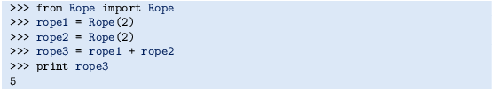
  As seen, the class also features a __str__ method for returning the number of knots on the rope.

• b) Equip the module file with a test function for verifying the implementation of the addition operator.

Filename: Rope.py.

Exercise 7.15 (Implement in-place += and -= operators)

As alternatives to the deposit and withdraw methods in class Account class from Sect. 7.2.1, we could use the operation += for deposit and -= for withdraw. Implement the += and -= operators, a __str__ method, and preferably a __repr__ method in class Account. Write a test_Account() function to verify the implementation of all functionality in class Account.

Hint

The special methods __iadd__ and __isub__ implement the += and -= operators, respectively. For instance, a -= p implies a call to a.__isub__(p). One important feature of __iadd__ and __isub__ is that they must return self to work properly, see the documentation of these methods in Chapter 3 of the Python Language Reference⁴.

Filename: Account4.

Exercise 7.16 (Implement a class for numerical differentiation)

A widely used formula for numerical differentiation of a function $f(x)$ takes the form

$$f^{\prime}(x)\approx{f(x+h)-f(x-h)\over 2h}\thinspace.$$

(7.8)

This formula usually gives more accurate derivatives than (7.1) because it applies a centered, rather than a one-sided, difference.

The goal of this exercise is to use the formula (7.8) to automatically differentiate a mathematical function $f(x)$ implemented as a Python function f(x). More precisely, the following code should work:

• a) Implement class Central and test that the code above works. Include an optional argument h to the constructor in class Central so that h in the approximation (7.8) can be specified.

• b) Write a test function test_Central() to verify the implementation. Utilize the fact that the formula (7.8) is exact for quadratic polynomials (provided h is not too small, then rounding errors in (7.8) require use of a (much) larger tolerance than the expected machine precision).

• c) Write a function table(f, x, h=1E-5) that prints a table of errors in the numerical derivative (7.8) applied to a function f at some points x. The argument f is a sympy expression for a function. This f object can be transformed to a Python function and fed to the constructor of class Central, and f can be used to compute the exact derivative symbolically. The argument x is a list or array of points x, and h is the h in (7.8).

Hint

The following session demonstrates how sympy can differentiate a mathematical expression and turn the result into a Python function:

• a) Organize the file with the class and functions such that it can be used a module.

Filename: Central.

Exercise 7.17 (Examine a program)

Consider this program file for computing a backward difference approximation to the derivative of a function f(x):

The output becomes

Is the approximation that bad, or are there bugs in the program?

Filename: find_errors_class.

Exercise 7.18 (Modify a class for numerical differentiation)

Make the two data attributes h and f of class Derivative from Sect. 7.3.2 protected as explained in Sect. 7.2.1. That is, prefix h and f with an underscore to tell users that these attributes should not be accessed directly. Add two methods get_precision() and set_precision(h) for reading and changing h. Make a separate test function for checking that the new class works as intended.

Filename: Derivative_protected.

Exercise 7.19 (Make a class for the Heaviside function)

• a) Use a class to implement the discontinuous Heaviside function (3.25) from Exercise 3.5 and the smoothed continuous version (3.26) from Exercise 3.5 such that the following code works:

  

• b) Extend class Heaviside such that array arguments are allowed:

  

Hint

Use ideas from Sect. 5.5.2.

• a) Extend class Heaviside such that it supports plotting:

  

Hint

Techniques from Sect. 5.4.1 must in the first case be used to return arrays x and y such that the discontinuity is exactly reproduced. In the continuous (smoothed) case, one needs to compute a sufficiently fine resolution (x) based on the eps parameter, e.g., 201/ϵ points in the interval $[-\epsilon,\epsilon]$, with a coarser set of coordinates outside this interval where the smoothed Heaviside function is almost constant, 0 or 1.

• a) Write a test function test_Heaviside() for verifying the result of the various methods in class Heaviside.

Filename: Heaviside_class.

Exercise 7.20 (Make a class for the indicator function)

The purpose of this exercise is the make a class implementation of the indicator function from Exercise 3.5. Let the implementation be based on expressing the indicator function in terms of Heaviside functions. Allow for an ϵ parameter in the calls to the Heaviside function, such that we can easily choose between a discontinuous and a smoothed, continuous version of the indicator function:

Note that if you build on the version of class Heaviside in Exercise 7.19b, any Indicator instance will accept array arguments too.

Filename: Indicator.

Exercise 7.21 (Make a class for piecewise constant functions)

The purpose of this exercise is to make a class implementation of a piecewise constant function, as defined in Exercise 3.5.

• a) Implement the minimum functionality such that the following code works:

  

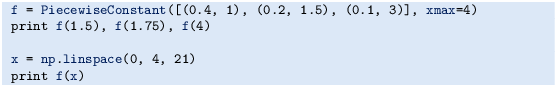
• b) Add a plot method to class PiecewiseConstant such that we can easily plot the graph of the function:

  

Filename: PiecewiseConstant.

Exercise 7.22 (Speed up repeated integral calculations)

The observant reader may have noticed that our Integral class from Sect. 7.3.3 is very inefficient if we want to tabulate or plot a function $F(x)=\int_{a}^{x}f(x)$ for several consecutive values of x: $x_{0}<x_{1}<\cdots<x_{m}$. Requesting $F(x_{k})$ will recompute the integral computed for $F(x_{k-1})$, and this is of course waste of computer work. Use the ideas from Sect. A.1.7 to modify the __call__ method such that if x is an array, assumed to contain coordinates of increasing value: $x_{0}<x_{1}<\cdots<x_{m}$, the method returns an array with $F(x_{0}),F(x_{1}),\ldots,F(x_{m})$ with the minimum computational work. Also write a test function to verify that the implementation is correct.

Hint

The n (n) parameter in the constructor of the Integral class can be taken as the total number of trapezoids (intervals) that are to be used to compute the final $F(x_{m})$ value. The integral over an interval $[x_{k},x_{k+1}]$ can then be computed by the trapezoidal function (or an Integral object) using an appropriate fraction of the n total trapezoids. This fraction can be $(x_{k+1}-x_{k})/(x_{m}-a)$ (i.e., $n_{k}=n(x_{k+1}-x_{k})/(x_{m}-a)$) or one may simply use a constant $n_{k}=n/m$ number of trapezoids for all the integrals over $[x_{k},x_{k+1}]$, $k=0,\ldots,m-1$.

Filename: Integral_eff.

Exercise 7.23 (Apply a class for polynomials)

The Taylor polynomial of degree N for the exponential function e^x is given by

$$p(x)=\sum_{k=0}^{N}{x^{k}\over k!}\thinspace.$$

Make a program that (i) imports class Polynomial from Sect. 7.3.7, (ii) reads x and a series of N values from the command line, (iii) creates a Polynomial object for each N value for computing with the given Taylor polynomial, and (iv) prints the values of $p(x)$ for all the given N values as well as the exact value e^x. Try the program out with x = 0.5,3,10 and N = 2,5,10,15,25.

Filename: Polynomial_exp.

Exercise 7.24 (Find a bug in a class for polynomials)

Go through this alternative implementation of class Polynomial from Sect. 7.3.7 and explain each line in detail:

The enumerate function, used in the __call__ method, enables us to iterate over a list somelist with both list indices and list elements: for index, element in enumerate(somelist). Write the code above in a file, and demonstrate that adding two polynomials does not work. Find the bug and correct it.

Filename: Polynomial_error.

Exercise 7.25 (Implement subtraction of polynomials)

Implement the special method __sub__ in class Polynomial from Sect. 7.3.7. Add a test for this functionality in function test_Polynomial.

Hint

Study the __add__ method in class Polynomial and treat the two cases, where the lengths of the lists in the polynomials differs, separately.

Filename: Polynomial_sub.

Exercise 7.26 (Test the functionality of pretty print of polynomials)

Verify the functionality of the __str__ method in class Polynomial from Sect. 7.3.7 by writing a new test function test_Polynomial_str().

Filename: Polynomial_test_str.

Exercise 7.27 (Vectorize a class for polynomials)

Introducing an array instead of a list in class Polynomial does not enhance the efficiency of the implementation unless the mathematical computations are also vectorized. That is, all explicit Python loops must be substituted by vectorized expressions.

• a) Go through class Polynomial.py and make sure the coeff attribute is always a numpy array with float elements.

• b) Update the test function test_Polynomial to make use of the fact that the coeff attribute is always a numpy array with float elements. Run test_Polynomial to check that the new implementation is correct.

• c) Vectorize the __add__ method by adding the common parts of the coefficients arrays and then appending the rest of the longest array to the result.

Hint

Appending an array a to an array b can be done by concatenate(a, b).

• a) Vectorize the __call__ method by observing that evaluation of a polynomial, $\sum_{i=0}^{n-1}c_{i}x^{i}$, can be computed as the inner product of two arrays: $(c_{0},\ldots,c_{n-1})$ and $(x^{0},x^{1},\ldots,x^{n-1})$. The latter array can be computed by x**p, where p is an array with powers $0,1,\ldots,n-1$, and x is a scalar.

• b) The differentiate method can be vectorized by the statements

  

  Show by hand calculations in a case where n is 3 that the vectorized statements produce the same result as the original differentiate method.

Filename: Polynomial_vec.

Remarks

The __mul__ method is more challenging to vectorize so you may leave this unaltered. Check that the vectorized versions of __add__, __call__, and differentiate work as intended by calling the test_Polynomial function.

Exercise 7.28 (Use a dict to hold polynomial coefficients)

Use a dictionary (instead of a list) for the coeff attribute in class Polynomial from Sect. 7.3.7 such that self.coeff[k] holds the coefficient of the x^k term. The advantage with a dictionary is that only the nonzero coefficients in a polynomial need to be stored.

• a) Implement a constructor and the __call__ method for evaluating the polynomial. The following demonstration code should work:

  

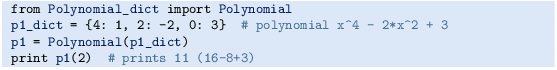
• b) Implement the __add__ method. The following demonstration code should work:

  

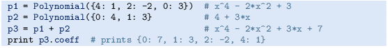
Hint

The structure of __add__ may be

• a) Implement the __sub__ method. The following demonstration code should work:

  

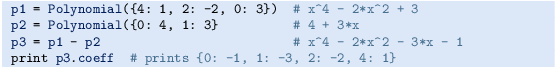
• b) Implement the __mul__ method. The following demonstration code should work:

  

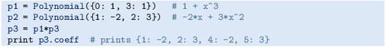
Hint

Study the __mul__ method in class Polynomial based on a list representation of the data in the polynomial and adapt to a dictionary representation.

• a) Write a test function for each of the methods __call__, __add__, and __mul__.

Filename: Polynomial_dict.

Exercise 7.29 (Extend class Vec2D to work with lists/tuples)

The Vec2D class from Sect. 7.4 supports addition and subtraction, but only addition and subtraction of two Vec2D objects. Sometimes we would like to add or subtract a point that is represented by a list or a tuple:

That is, a list or a tuple must be allowed in the right or left operand. Implement such an extension of class Vec2D.

Hint

Ideas are found in Sects. 7.5.3 and 7.5.5.

Filename: Vec2D_lists.

Exercise 7.30 (Extend class Vec2D to 3D vectors)

Extend the implementation of class Vec2D from Sect. 7.4 to a class Vec3D for vectors in three-dimensional space. Add a method cross for computing the cross product of two 3D vectors.

Filename: Vec3D.

Exercise 7.31 (Use NumPy arrays in class Vec2D)

The internal code in class Vec2D from Sect. 7.4 can be valid for vectors in any space dimension if we represent the vector as a NumPy array in the class instead of separate variables x and y for the vector components. Make a new class Vec where you apply NumPy functionality in the methods. The constructor should be able to treat all the following ways of initializing a vector:

Hint

In the constructor, use variable number of arguments as described in Sect. H.7. All arguments are then available as a tuple, and if there is only one element in the tuple, it should be an array, list, or tuple you can send through asarray to get a NumPy array. If there are many arguments, these are coordinates, and the tuple of arguments can be transformed by array to a NumPy array. Assume in all operations that the involved vectors have equal dimension (typically that other has the same dimension as self). Recall to return Vec objects from all arithmetic operations, not NumPy arrays, because the next operation with the vector will then not take place in Vec but in NumPy. If self.v is the attribute holding the vector as a NumPy array, the addition operator will typically be implemented as

Filename: Vec.

Exercise 7.32 (Impreciseness of interval arithmetics)

Consider the function $f(x)=x/(1+x)$ on $[1,2]$. Find the variation of f over $[1,2]$. Use interval arithmetics from Sect. 7.7.2 to compute the variation of f when $x\in[1,2]$.

Filename: interval_arithmetics.

Remarks

In this case, interval arithmetics overestimates the variation in f. The reason is that x occurs more than once in the formula for f (the so-called dependency problem⁵).

Exercise 7.33 (Make classes for students and courses)

Use classes to reimplement the summarizing problem in Sect. 6.7.2. More precisely, introduce a class Student and a class Course. Find appropriate attributes. The classes should have a __str__ method for pretty-printing of the contents.

Filename: Student_Course.

Exercise 7.34 (Find local and global extrema of a function)

Extreme points of a function $f(x)$ are normally found by solving $f^{\prime}(x)=0$. A much simpler method is to evaluate $f(x)$ for a set of discrete points in the interval $[a,b]$ and look for local minima and maxima among these points. We work with $n+1$ equally spaced points $a=x_{0}<x_{1}<\cdots<x_{n}=b$, $x_{i}=a+ih$, $h=(b-a)/n$.

First we find all local extreme points in the interior of the domain. Local minima are recognized by

$$f(x_{i-1})> f(x_{i})<f(x_{i+1}),\quad i=1,\ldots,n-1\thinspace.$$

Similarly, at a local maximum point x_i we have

$$f(x_{i-1})<f(x_{i})> f(x_{i+1}),\quad i=1,\ldots,n-1\thinspace.$$

Let $P_{\min}$ be the set of x values for local minima and $F_{\min}$ the set of the corresponding $f(x)$ values at these minima. Two sets $P_{\max}$ and $F_{\max}$ are defined correspondingly for the maxima.

The boundary points $x=a$ and $x=b$ are for algorithmic simplicity also defined as local extreme points: $x=a$ is a local minimum if $f(a)<f(x_{1})$, and a local maximum otherwise. Similarly, $x=b$ is a local minimum if $f(b)<f(x_{n-1})$, and a local maximum otherwise. The end points a and b and the corresponding function values must be added to the sets $P_{\min},P_{\max},F_{\min},F_{\max}$.

The global maximum point is defined as the x value corresponding to the maximum value in $F_{\max}$. The global minimum point is the x value corresponding to the minimum value in $F_{\min}$.

• a) Make a class MinMax with the following functionality:

  • __init__ takes $f(x)$, a, b, and n as arguments, and calls a method _find_extrema to compute the local and global extreme points.

  • _find_extrema implements the algorithm above for finding local and global extreme points, and stores the sets $P_{\min},P_{\max},F_{\min},F_{\max}$ as list attributes in the (self) instance.

  • get_global_minimum returns the global minimum point as a pair $(x,f(x))$.

  • get_global_maximum returns the global maximum point as a pair $(x,f(x))$.

  • get_all_minima returns a list or array of all $(x,f(x))$ minima.

  • get_all_maxima returns a list or array of all $(x,f(x))$ maxima.

  • __str__ returns a string where a nicely formatted table of all the min/max points are listed, plus the global extreme points.

  Here is a sample code using class MinMax:

  

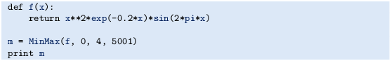
  The output becomes

  

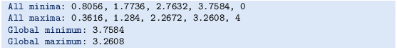
  Make sure that the program also works for functions without local extrema, e.g., linear functions $f(x)=ax+b$.

• b) The algorithm sketched above finds local extreme points x_i, but all we know is that the true extreme point is in the interval $(x_{i-1},x_{i+1})$. A more accurate algorithm may take this interval as a starting point and run a Bisection method (see Sect. 4.11.2) to find the extreme point $\bar{x}$ such that $f^{\prime}(\bar{x})=0$. Add a method _refine_extrema in class MinMax, which goes through all the interior local minima and maxima and solves $f^{\prime}(\bar{x})=0$. Compute $f^{\prime}(x)$ using the Derivative class (Sect. 7.3.2 with $h\ll x_{i+1}-x_{i-1}$.

Filename: minmaxf.

Exercise 7.35 (Find the optimal production for a company)

The company PROD produces two different products, P${}_{1}$ and P${}_{2}$, based on three different raw materials, $\mbox{M}_{1}$, $\mbox{M}_{2}$ and $\mbox{M}_{3}$. The following table shows how much of each raw material $\mbox{M}_{i}$ that is required to produce a single unit of each product P${}_{j}$:

For instance, to produce one unit of $\mbox{P}_{2}$ one needs 1 unit of $\mbox{M}_{1}$, 3 units of $\mbox{M}_{2}$ and 4 units of $\mbox{M}_{3}$. Furthermore, PROD has available 100, 80 and 150 units of material $\mbox{M}_{1}$, $\mbox{M}_{2}$ and $\mbox{M}_{3}$ respectively (for the time period considered). The revenue per produced unit of product $\mbox{P}_{1}$ is 150 NOK, and for one unit of $\mbox{P}_{2}$ it is 175 NOK. On the other hand the raw materials $\mbox{M}_{1}$, $\mbox{M}_{2}$ and $\mbox{M}_{3}$ cost 10, 17 and 25 NOK per unit, respectively. The question is: how much should PROD produce of each product? We here assume that PROD wants to maximize its net revenue (which is revenue minus costs).

• a) Let x and y be the number of units produced of product $\mbox{P}_{1}$ and $\mbox{P}_{2}$, respectively. Explain why the total revenue $f(x,y)$ is given by

  $$f(x,y)=150x-(10\cdot 2+17\cdot 5)x+175y-(10\cdot 1+17\cdot 3+25\cdot 4)y$$

  and simplify this expression. The function $f(x,y)$ is linear in x and y (make sure you know what linearity means).

• b) Explain why PROD’s problem may be stated mathematically as follows:

  $$\begin{array}[]{lrrrrr}\mbox{\rm maximize}&\multicolumn{3}{c}{f(x,y)}\\ \mbox{\rm subject to}&\\ &2x&+&y&\leq&100\\ &5x&+&3y&\leq&80\\ &&&4y&\leq&150\\ &&\multicolumn{4}{l}{x\geq 0,y\geq 0.}\end{array}$$

  (7.9)

  This is an example of a linear optimization problem.

• c) The production $(x,y)$ may be considered as a point in the plane. Illustrate geometrically the set T of all such points that satisfy the constraints in model (7.9). Every point in this set is called a feasible point.

Table 2

Hint

For every inequality determine first the straight line obtained by replacing the inequality by equality. Then, find the points satisfying the inequality (a half-plane), and finally, intersect these half-planes.

• a) Make a program for drawing the straight lines defined by the inequalities. Each line can be written as $ax+by=c$. Let the program read each line from the command line as a list of the a, b, and c values. In the present case the command-line arguments will be

  

Hint

Perform an eval on the elements of sys.argv[1:] to get a, b, and c for each line as a list in the program.

• a) Let α be a positive number and consider the level set of the function f, defined as the set

  $$L_{\alpha}=\{(x,y)\in T:f(x,y)=\alpha\}.$$

  This set consists of all feasible points having the same net revenue α. Extend the program with two new command-line arguments holding p and q for a function $f(x,y)=px+qy$. Use this information to compute the level set lines $y=\alpha/q-px/q$, and plot the level set lines for some different values of α (use the α value in the legend for each line).

• b) Use what you saw in e) to solve the problem (7.9) geometrically. This solution is called an optimal solution.

Hint

How large can you choose α such that $L_{\alpha}$ is nonempty?

• a) Assume that we have other values on the revenues and costs than the actual numbers in a). Explain why (7.9), with these new parameter values, still has an optimal solution lying in a corner point of T. Extend the program to calculate all the corner points of a region T in the plane determined by the linear inequalities like those listed above. Moreover, the program shall compute the maximum of a given linear function $f(x,y)=ax+by$ over T by calculating the function values in the corner points and finding the smallest function value.

Filename: optimization.