Dictionaries and Strings

Abstract

The present chapter addresses many techniques for interpreting information in files and storing the data in convenient Python objects for further data analysis. A particularly handy object for many purposes is the dictionary, which maps objects to objects, very often strings to various kinds of data that later can be looked up through the strings. Section 6.1 is devoted to dictionaries.

Information in files often appear as pure text, so to interpret and extract data from files it is sometimes necessary to carry out sophisticated operations on the text. Python strings have many methods for performing such operations, and the most important functionality is described in Sect. 6.2.

The World Wide Web is full of information and scientific data that may be useful to access from a program. Section 6.3 tells you how to read web pages from a program and interpret the contents using string operations.

Working with data often involves spreadsheets. Python programs not only need to extract data from spreadsheet files, but it can be advantageous and convenient to actually to the data processing in a Python program rather than in a spreadsheet program like Microsoft Excel or LibreOffice. Section 6.4 goes through relevant techniques for reading and writing files in the common CSV format for spreadsheets.

The present chapter builds on fundamental programming concepts such as loops, lists, arrays, if tests, command-line arguments, and curve plotting. The folder src/files contains all the relevant program example files and associated data files.

The present chapter addresses many techniques for interpreting information in files and storing the data in convenient Python objects for further data analysis. A particularly handy object for many purposes is the dictionary, which maps objects to objects, very often strings to various kinds of data that later can be looked up through the strings. Section 6.1 is devoted to dictionaries.

Information in files often appear as pure text, so to interpret and extract data from files it is sometimes necessary to carry out sophisticated operations on the text. Python strings have many methods for performing such operations, and the most important functionality is described in Sect. 6.2.

The World Wide Web is full of information and scientific data that may be useful to access from a program. Section 6.3 tells you how to read web pages from a program and interpret the contents using string operations.

Working with data often involves spreadsheets. Python programs not only need to extract data from spreadsheet files, but it can be advantageous and convenient to actually to the data processing in a Python program rather than in a spreadsheet program like Microsoft Excel or LibreOffice. Section 6.4 goes through relevant techniques for reading and writing files in the common CSV format for spreadsheets.

The present chapter builds on fundamental programming concepts such as loops, lists, arrays, if tests, command-line arguments, and curve plotting. The folder src/filesFootnote

http://tinyurl.com/pwyasaa/files

contains all the relevant program example files and associated data files.

6.1 Dictionaries

So far in the book we have stored information in various types of objects, such as numbers, strings, list, and arrays. A dictionary is a very flexible object for storing various kind of information, and in particular when reading files. It is therefore time to introduce the popular dictionary type.

A list is a collection of objects indexed by an integer going from 0 to the number of elements minus one. Instead of looking up an element through an integer index, it can be more handy to use a text. Roughly speaking, a list where the index can be a text is called a dictionary in Python. Other computer languages use other names for the same thing: HashMap, hash, associative array, or map.

6.1.1 Making Dictionaries

Suppose we need to store the temperatures from three cities: Oslo, London, and Paris. For this purpose we can use a list,

but then we need to remember the sequence of cities, e.g., that index 0 corresponds to Oslo, index 1 to London, and index 2 to Paris. That is, the London temperature is obtained as temps[1]. A dictionary with the city name as index is more convenient, because this allows us to write temps[’London’] to look up the temperature in London. Such a dictionary is created by one of the following two statements

Additional text-value pairs can be added when desired. We can, for instance, write

The temps dictionary has now four text-value pairs, and a print temps yields

6.1.2 Dictionary Operations

The string ‘‘indices’’ in a dictionary are called keys. To loop over the keys in a dictionary d, one writes for key in d: and works with key and the corresponding value d[key] inside the loop. We may apply this technique to write out the temperatures in the temps dictionary from the previous paragraph:

We can check if a key is present in a dictionary by the syntax if key in d:

Writing key in d yields a standard boolean expression, e.g.,

The keys and values can be extracted as lists from a dictionary:

An important feature of the keys method in dictionaries is that the order of the returned list of keys is unpredictable. If you need to traverse the keys in a certain order, you can sort the keys. A loop over the keys in the temps dictionary in alphabetic order is written as

Python also has a special dictionary type OrderedDict where the key-value pairs has a specific order, see Sect. 6.1.4.

A key-value pair can be removed by del d[key]:

Sometimes we need to take a copy of a dictionary:

Note that if two variables refer to the same dictionary and we change the contents of the dictionary through either of the variables, the change will be seen in both variables:

To avoid that temps is affected by adding a new key-value pair to t1, t1 must be a copy of temps.

Remark

In Python version 2.x, temps.keys() returns a list object while in Python version 3.x, temps.keys() only enables iterating over the keys. To write code that works with both versions one can use list(temps.keys()) in the cases where a list is really needed and just temps.keys() in a for loop over the keys.

6.1.3 Example: Polynomials as Dictionaries

Python objects that cannot change their contents are known as immutable data types and consist of int, float, complex, str, and tuple. Lists and dictionaries can change their contents and are called mutable objects.

The keys in a dictionary are not restricted to be strings. In fact, any immutable Python object can be used as key. For example, if you want a list as key, it cannot be used since lists can change their contents are hence mutable objects, but a tuple will do, since it is immutable.

A common type of key in dictionaries is integers. Next we shall explain how dictionaries with integers as key provide a handy way of representing polynomials. Consider the polynomial

$$p(x)=-1+x^{2}+3x^{7}\thinspace.$$

The data associated with this polynomial can be viewed as a set of power-coefficient pairs, in this case the coefficient −1 belongs to power 0, the coefficient 1 belongs to power 2, and the coefficient 3 belongs to power 7. A dictionary can be used to map a power to a coefficient:

A list can, of course, also be used, but in this case we must fill in all the zero coefficients too, since the index must match the power:

The advantage with a dictionary is that we need to store only the non-zero coefficients. For the polynomial $1+x^{100}$ the dictionary holds two elements while the list holds 101 elements (see Exercise 6.10).

The following function can be used to evaluate a polynomial represented as a dictionary:

The poly argument must be a dictionary where poly[power] holds the coefficient associated with the term x**power.

A more compact implementation can make use of Python’s sum function to sum the elements of a list:

That is, we first make a list of the terms in the polynomial using a list comprehension, and then we feed this list to the sum function. We can in fact drop the brackets and storing all the poly[power]*x**power numbers in a list, because sum can directly add elements of an iterator (like for power in poly):

Be careful with redefining variables!

The name sum appears in both eval_poly_dict and eval_poly_dict2. In the former, sum is a float object, and in the latter, sum is a built-in Python function. When we set sum=0.0 in the first implementation, we bind the name sum to a new float object, and the built-in Python function associated with the name sum is then no longer accessible inside the eval_poly_dict function. (Actually, this is not strictly correct, because sum is a local variable while the built-in Python sum function is associated with a global name sum, which can always be reached through globals()[’sum’].) Outside the eval_poly_dict function, nevertheless, sum will be Python’s summation function and the local sum variable inside the eval_poly_dict function is destroyed.

As a rule of thumb, avoid using sum or other names associated with frequently used functions as new variables unless you are in a very small function (like eval_poly_dict) where there is no danger that you need the original meaning of the name.

With a list instead of dictionary for representing the polynomial, a slightly different evaluation function is needed:

If there are many zeros in the poly list, eval_poly_list must perform all the multiplications with the zeros, while eval_poly_dict computes with the non-zero coefficients only and is hence more efficient.

Another major advantage of using a dictionary to represent a polynomial rather than a list is that negative powers are easily allowed, e.g.,

can represent $\frac{1}{2}x^{-3}+2x^{4}$. With a list representation, negative powers require much more book-keeping. We may, for example, set

and remember that p[i] is the coefficient associated with the power i-3. In particular, the eval_poly_list function will no longer work for such lists, while the eval_poly_dict function works also for dictionaries with negative keys (powers).

There is a dictionary counterpart to list comprehensions, called dictionary comprehensions, for quickly generating parameterized key-value pairs with a for loop. Such a construction is convenient to generate the coefficients in a polynomial:

The d dictionary now contains the power-coefficient pairs of the Taylor polynomial of degree n for $e^{-x}$. (Note the use of float to avoid integer division.)

You are now encouraged to solve Exercise 6.11 to become more familiar with the concept of dictionaries.

6.1.4 Dictionaries with Default Values and Ordering

Dictionaries with default values

Looking up keys that are not present in the dictionary requires special treatment. Consider a polynomial dictionary of the type introduced in Sect. 6.1.3. Say we have $2x^{-3}-1.5x^{-1}-2x^{2}$ represented by

If the code tries to look up p1[1], this operation results in a KeyError since 1 is not a registered key in p1. We therefore need to do either

or use

where p1.get returns p1[key] if key in p1 and the default value 0.0 if not. A third possibility is to work with a dictionary with a default value:

The p2 can be indexed by any key, and for unregistered keys the polynomial_coeff_default function is called to provide a value. This must be a function without arguments. Usually, a separate function is never made, but either a type is inserted or a lambda function. The example above is equivalent to

In the latter case float() is called for each unknown key, and float() returns a float object with zero value. Now we can look up p2[1] and get the default value 0. It must be remarked that this key is then a part of the dictionary:

Ordered dictionaries

The elements of a dictionary have an undefined order. For example,

One can control the order by sorting the keys, either by the default sorting (alphabetically for string keys, ascending order for number keys):

The sorted function also accept an optional argument where the user can supply a function that sorts two keys (see Exercise 3.5).

However, Python features a dictionary type that preserves the order of the keys as they were registered:

Here is an example with dates as keys where the order is important.

The order of the keys in the loop is not the right registered order, but this is easily achieved by OrderedDict

A comment on alternative solutions should be made here. Trying to sort the data dictionary when it is an ordinary dict object does not help, as by default the sorting will be alphabetically, resulting in the sequence ’Feb 2’, ’Jan 16’, and ’Jan 2’. What does help, however, is to use Python’s datetime objects as keys reflecting dates, since these objects will be correctly sorted. A datetime object can be created from a string like ’Jan 2, 2017’ using a special syntax (see the module documentation). The relevant code is

Printing out in sorted order gives the right sequence of dates:

The time is automatically part of a datetime object and set to 00:00:00 when not specified.

While OrderedDict provides a simpler and shorter solution to keeping keys (here dates) in the right order in a dictionary, using datetime objects for dates has many advantages: dates can be formatted and written out in various ways, counting days between two dates is easy (see Sect. A.1.1), calculating the corresponding week number and name of the weekday is supported, to mention some functionality.

6.1.5 Example: Storing File Data in Dictionaries

Problem

The file files/densities.dat contains a table of densities of various substances measured in $\hbox{g}/\hbox{cm}^{3}$:

In a program we want to access these density data. A dictionary with the name of the substance as key and the corresponding density as value seems well suited for storing the data.

Solution

We can read the densities.dat file line by line, split each line into words, use a float conversion of the last word as density value, and the remaining one or two words as key in the dictionary.

This code is found in the file density.py. With string operations from Sect. 6.2.1 we can avoid the special treatment of one or two words in the name of the substance and achieve simpler and more general code, see Exercise 6.3.

6.1.6 Example: Storing File Data in Nested Dictionaries

Problem

We are given a data file with measurements of some properties with given names (here A, B, C …). Each property is measured a given number of times. The data are organized as a table where the rows contain the measurements and the columns represent the measured properties:

The word no stands for no data, i.e., we lack a measurement. We want to read this table into a dictionary data so that we can look up measurement no. i of (say) property C as data[’C’][i]. For each property p, we want to compute the mean of all measurements and store this as data[p][’mean’].

Algorithm

The algorithm for creating the data dictionary goes as follows:

• examine the first line: split it into words and initialize a dictionary with the property names as keys and empty dictionaries as values

• for each of the remaining lines in the file

  • split the line into words

  • for each word after the first

    • if the word is not no:

      • transform the word to a real number and store the number in the relevant dictionary

Implementation

A new aspect needed in the solution is nested dictionaries, that is, dictionaries of dictionaries. The latter topic is first explained, via an example:

Observe here that the value of d[’key1’] is a dictionary, which we can index with its keys key1 and key2:

In other words, repeated indexing works for nested dictionaries as for nested lists. The repeated indexing does not apply to d[’key2’] since that value is just an integer:

When we have understood the concept of nested dictionaries, we are in a position to present a complete code that solves our problem of loading the tabular data in the file table.dat into a nested dictionary data and computing mean values. First, we list the program, stored in the file table2dict.py, and display the program’s output. Thereafter, we dissect the code in detail.

The corresponding output from this program becomes

To view the nested data dictionary, we may insert

which produces something like

Dissection

To understand a computer program, you need to understand what the result of every statement is. Let us work through the code, almost line by line, and see what it does.

First, we load all the lines of the file into a list of strings called lines. The first_line variable refers to the string

We split this line into a list of words, called properties, which then contains

With each of these property names we associate a dictionary with the measurement number as key and the property value as value, but first we must create these ‘‘inner’’ dictionaries as empty before we can add the measurements:

The first pass in the for loop picks out the string

as the line variable. We split this line into words, the first word (words[0]) is the measurement number, while the rest words[1:] is a list of property values, here named values. To pair up the right properties and values, we loop over the properties and values lists simultaneously:

Recall that some values may be missing and we drop to record that value (we could, alternatively, set the value to None). Because the values list contains strings (words) read from the file, we need to explicitly transform each string to a float number before we can compute with the values.

After the for line in lines[1:] loop, we have a dictionary data of dictionaries where all the property values are stored for each measurement number and property name. Figure 6.1 shows a graphical representation of the data dictionary.

Fig. 6.1

Illustration of the nested dictionary created in the table2dict.py program

It remains to compute the average values. For each property name p, i.e., key in the data dictionary, we can extract the recorded values as the list data[p].values() and simply send this list to Python’s sum function and divide by the number of measured values for this property, i.e., the length of the list:

Alternatively, we can write an explicit loop to compute the average:

When we want to look up a measurement no. n of property B, we must recall that this particular measurement may be missing so we must do a test if n is key in the dictionary data[p]:

6.1.7 Example: Reading and Plotting Data Recorded at Specific Dates

Problem

We want to compare the evolution of the stock prices of some giant companies in the computer industry: Microsoft, Apple, and Google. Relevant data files for stock prices can be downloaded from http://finance.yahoo.com. Fill in the company’s name and click on Search Finance in the top bar of this page and choose Historical Prices in the left pane. On the resulting web page one can specify start and end dates for the historical prices of the stock. The default values were used in this example. Ticking off Monthly values and clicking Get Prices result in a table of stock prices for each month since the stock was introduced. The table can be downloaded as a spreadsheet file in CSV format, typically looking like

The file format is simple: columns are separated by comma, the first line contains column headings, and the data lines have the date in the first column and various measures of stock prices in the next columns. Reading about the meaning of the various data on the Yahoo! web pages reveals that our interest concerns the final column (as these prices are adjusted for splits and dividends). Three relevant data files can be found in the folder src/filesFootnote

http://tinyurl.com/pwyasaa/files

with the names stockprices_X.csv, where X is Microsoft, Apple, or Google.

The task is visually illustrate the historical, relative stock market value of these companies. For this purpose it is natural to scale the prices of a company’s stock to start at a unit value when the most recent company entered the market. Since the date of entry varies, the oldest data point can be skipped such that all data points correspond to the first trade day every month.

Solution

There are two major parts of this problem: reading the file and plotting the data. The reading part is quite straightforward, while the plotting part needs some special considerations since the x values in the plot are dates and not real numbers. In the forthcoming text we solve the individual subproblems one by one, showing the relevant Python snippets. The complete program is found in the file stockprices.py.

We start with the reading part. Since the reading will be repeated for several companies, we create a function for extracting the relevant data for a specific company. These data cover the dates in column 1 and the stock prices in the last column. Since we want to plot prices versus dates, it will be convenient to turn the dates into date objects. In more detail the algorithms has the following points:

• 1. open the file

• 2. create two empty lists, dates and prices, for collecting the data

• 3. read the first line (of no interest)

• 4. for each line in the rest of the file:

  • a) split the line wrt. comma into words

  • b) append the first word to the dates list

  • c) append the last word to the prices list

• 5. reverse the lists (oldest date first)

• 6. convert date strings to datetime objects

• 7. convert prices list to float array for computations

• 8. return dates and prices, except for the first (oldest) data point

There are a couple of additional points to consider. First, the words on a line are strings, and at least the prices (last word) should be converted to a float. Second, the recipe for converting dates like ’2008-02-04’ to date (or datetime) objects goes as

The nice thing with date and datetime object is that we can compute with them and in particular used them in plotting with Matplotlib.

We can now translate the algorithm to Python code:

Although we work with three companies in this example, it is easy and almost always a good idea to generalize the program to an arbitrary number of companies. All we assume is that their stock prices are in files with names of the form stockprices_X.csv, where X is the company name. With aid of the function call glob.glob(’stockprices_*.csv’) we get a list of all such files. By looping over this list, extracting the company name, and calling read_file, we can store the dates and corresponding prices in dictionaries dates and prices, indexed by the company name:

The next step is to normalize the prices such that they coincide on a certain date. We pick this date as the first month we have data for the youngest company. In lists of date or datetime objects, we can use Python’s max and min functions to extract the newest and oldest date.

The normalized prices vary a lot, so to see the development over 30 years better, we decide to take the logarithm of the prices. The plotting procedure is somewhat involved so the reader should take the coming code more as a recipe than as a sequence of statement to really understand:

Figure 6.2 shows the resulting plot. We observe that the normalized prices coincide when Google entered the market, here at Sep 1, 2004. Note that there is a log scale on the vertical axis. You may want to plot the real normalized prices to get a stronger impression of the significant recent rise in value, especially for Apple.

Fig. 6.2

The evolution of stock prices for three companies

6.2 Strings

Many programs need to manipulate text. For example, when we read the contents of a file into a string or list of strings (lines), we may want to change parts of the text in the string(s) – and maybe write out the modified text to a new file. So far in this chapter we have converted parts of the text to numbers and computed with the numbers. Now it is time to learn how to manipulate the text strings themselves.

6.2.1 Common Operations on Strings

Python has a rich set of operations on string objects. Some of the most common operations are listed below.

Substring specification

The expression s[i:j] extracts the substring starting with character number i and ending with character number j-1 (similarly to lists, 0 is the index of the first character):

A negative upper index counts, as usual, from the right such that s[-1] is the last element, s[-2] is the next last element, and so on.

Searching for substrings

The call s.find(s1) returns the index where the substring s1 first appears in s. If the substring is not found, −1 is returned.

Sometimes the aim is to just check if a string is contained in another string, and then we can use the syntax:

Here is a typical use of the latter construction in an if test:

Two other convenient methods for checking if a string starts with or ends with a specified string are startswith and endswith:

Substitution

The call s.replace(s1, s2) replaces substring s1 by s2 everywhere in s:

A variant of the last example, where several string operations are put together, consists of replacing the text before the first colon:

Take a break at this point and convince yourself that you understand how we specify the substring to be replaced!

String splitting

The call s.split() splits the string s into words separated by whitespace (space, tabulator, or newline):

Splitting a string s into words separated by a text t can be done by s.split(t). For example, we may split with respect to colon:

We know that s contains a city name, a colon, a temperature, and then C:

With s.splitlines(), a multi-line string is split into lines (very useful when a file has been read into a string and we want a list of lines):

Upper and lower case

s.lower() transforms all characters to their lower case equivalents, and s.upper() performs a similar transformation to upper case letters:

Strings are constant

A string cannot be changed, i.e., any change always results in a new string. Replacement of a character is not possible:

If we want to replace s[18], a new string must be constructed, for example by keeping the substrings on either side of s[18] and inserting a ’5’ in between:

Strings with digits only

One can easily test whether a string contains digits only or not:

Whitespace

We can also check if a string contains spaces only by calling the isspace method. More precisely, isspace tests for whitespace, which means the space character, newline, or the TAB character:

The isspace is handy for testing for blank lines in files. An alternative is to strip first and then test for an empty string:

Stripping off leading and/or trailing spaces in a string is sometimes useful:

Joining strings

The opposite of the split method is join, which joins elements in a list of strings with a specified delimiter in between. That is, the following two types of statements are inverse operations:

An example on using join may be

As an illustration of the usefulness of split and join, we want to remove the first two words on a line. This task can be done by first splitting the line into words and then joining the words of interest:

There are many more methods in string objects. All methods are described in the String Methods³ section of the Python Standard Library online document.

6.2.2 Example: Reading Pairs of Numbers

Problem

Suppose we have a file consisting of pairs of real numbers, i.e., text of the form $(a,b)$, where a and b are real numbers. This notation for a pair of numbers is often used for points in the plane, vectors in the plane, and complex numbers. A sample file may look as follows:

The file can be found as read_pairs1.dat. Our task is to read this text into a nested list pairs such that pairs[i] holds the pair with index i, and this pair is a tuple of two float objects. We assume that there are no blanks inside the parentheses of a pair of numbers (we rely on a split operation, which would otherwise not work).

Solution

To solve this programming problem, we can read in the file line by line; for each line: split the line into words (i.e., split with respect to whitespace); for each word: strip off the parentheses, split with respect to comma, and convert the resulting two words to floats. Our brief algorithm can be almost directly translated to Python code:

This code is available in the file read_pairs1.py. The with statement is the modern Python way of reading files, see Sect. 4.5.2, with the advantage that we do not need to think about closing the file. Figure 6.3 shows a snapshot of the state of the variables in the program after having treated the first line. You should explain each line in the program to yourself, and compare your understanding with the figure.

Fig. 6.3

Illustration of the variables in the read_pairs.py program after the first pass in the loop over words in the first line of the data file

The output from the program becomes

We remark that our solution to this programming problem relies heavily on the fact that spaces inside the parentheses are not allowed. If spaces were allowed, the simple split to obtain the pairs on a line as words would not work. What can we then do?

We can first strip off all blanks on a line, and then observe that the pairs are separated by the text ’)(’. The first and last pair on a line will have an extra parenthesis that we need to remove. The rest of code is similar to the previous code and can be found in read_pairs2.py:

The program can be tested on the file read_pairs2.dat:

A third approach is to notice that if the pairs were separated by commas,

the file text is very close to the Python syntax of a list of 2-tuples. We only miss the enclosing brackets:

Running eval on this text will automatically produce the list object we want to construct! All we need to do is to read the file into a string, add a comma after every right parenthesis, add opening and closing bracket, and call eval (program read_pairs3.py):

In general, it is a good idea to construct file formats that are as close as possible to valid Python syntax such that one can take advantage of the eval or exec functions to turn text into ‘‘live objects’’.

6.2.3 Example: Reading Coordinates

Problem

Suppose we have a file with coordinates $(x,y,z)$ in three-dimensional space. The file format looks as follows:

The goal is to read this file and create a list with (x,y,z) 3-tuples, and thereafter convert the nested list to a two-dimensional array with which we can compute.

Note that there is sometimes a space between the = signs and the following number and sometimes not. Splitting with respect to space and extracting every second word is therefore not an option. We shall present three solutions.

Solution 1: substring extraction

The file format looks very regular with the x=, y=, and z= texts starting in the same columns at every line. By counting characters, we realize that the x= text starts in column 2, the y= text starts in column 16, while the z= text starts in column 31. Introducing

the three numbers in a line string are obtained as the substrings

The following code, found in file file2coor_v1.py, creates the coor array with shape $(n,3)$, where n is the number of $(x,y,z)$ coordinates.

The print statement inside the loop is always wise to include when doing string manipulations, simply because counting indices for substring limits quickly leads to errors. Running the program, the output from the loop looks like this

for the first line in the file. The double quotes show the exact extent of the extracted coordinates. Note that the last quote appears on the next line. This is because line has a newline at the end (this newline must be there to define the end of the line), and the substring line[z_start:] contains the newline at the of line. Writing line[z_start:-1] would leave the newline out of the z coordinate. However, this has no effect in practice since we transform the substrings to float, and an extra newline or other blanks make no harm.

The coor object at the end of the program has the value

Solution 2: string search

One problem with the solution approach above is that the program will not work if the file format is subject to a change in the column positions of x=, y=, or z=. Instead of hardcoding numbers for the column positions, we can use the find method in string objects to locate these column positions:

The rest of the code is similar to the complete program listed above, and the complete code is stored in the file file2coor_v2.py.

Solution 3: string split

String splitting is a powerful tool, also in the present case. Let us split with respect to the equal sign. The first line in the file then gives us the words

We throw away the first word, and strip off the last character in the next word. The final word can be used as is. The complete program is found in the file file2coor_v3.py and looks like

More sophisticated examples of string operations appear in Sect. 6.3.4.

6.3 Reading Data from Web Pages

Python has a module urllib which makes it possible to read data from a web page as easily as we can read data from an ordinary file. (In principle this is true, but in practice the text in web pages tend to be much more complicated than the text in the files we have treated so far.) Before we do this, a few concepts from the Internet world must be touched.

6.3.1 About Web Pages

Web pages are viewed with a web browser. There are many browsers: Firefox, Internet Explorer, Safari, Opera, and Google Chrome to mention the most famous. Any web page you visit is associated with an address, usually something like

This type of web address is called a URL (Uniform Resource Locator) or URI (Uniform Resource Identifier). (We stick to the term URL in this book because Python’s tools for accessing resources on the Internet have url as part of module and function names.) The graphics you see in a web browser, i.e., the web page you see with your eyes, is produced by a series of commands that specifies the text on the page, the images, buttons to be pressed, etc. Roughly speaking, these commands are like statements in computer programs. The commands are stored in a text file and follow rules in a language, exactly as you are used to when writing statements in a programming language.

The common language for defining web pages is HTML. A web page is then simply a text file with text containing HTML commands. Instead of a physical file, the web page can also be the output text from a program. In that case the URL is the name of the program file.

The web browser interprets the text and the HTML commands, and then decides how to display the information visually. Let us demonstrate this for a very simple web page shown in Fig. 6.4. This page was produced by the following text with embedded HTML commands:

Fig. 6.4

Example of what a very simple HTML file looks like in a web browser

A typical HTML command consists of an opening and a closing tag. For example, emphasized text is specified by enclosing the text inside em (emphasize) tags:

The opening tag is enclosed in less than and greater than signs, while the closing tag has an additional forward slash before the tag name.

In the HTML file we see an opening and closing html tag around the whole text in the file. Similarly, there is a pair of body tags, where the first one also has a parameter bgcolor which can be used to specify a background color in the web page. Section headlines are specified by enclosing the headline text inside h1 tags. Subsection headlines apply h2 tags, which results in a smaller font compared with h1 tags. Comments appear inside <!-- and -->. Links to other web pages are written inside a tags, with an argument href for the link’s web address. Lists apply the ul (unordered list) tag, while each item is written with just an opening tag li (list item), but no closing tag is necessary. Images are also specified with just an opening tag having name img, and the image file is given as a file name or URL of a file, enclosed in double quotes, as the src parameter.

The ultra-quick HTML course in the previous paragraphs gives a glimpse of how web pages can be constructed. One can either write the HTML file by hand in a pure text editor, or one can use programs such as Dream Weaver to help design the page graphically in a user-friendly environment, and then the program can automatically generate the right HTML syntax in files.

6.3.2 How to Access Web Pages in Programs

Why is it useful to know some HTML and how web pages are constructed? The reason is that the web is full of information that we can get access to through programs and use in new contexts. What we can get access to is not the visual web page you see, but the underlying HTML file. The information you see on the screen appear in text form in the HTML file, and by extracting text, we can get hold of the text’s information in a program.

Given the URL as a string stored in a variable, there are two ways of accessing the HTML text in a Python program:

Alternative 1

Download the HTML file and store it as a local file with a given name, say webpage.html:

Alternative 2

Open the HTML file as a file-like object:

This infile object has methods such as read, readline, and readlines.

6.3.3 Example: Reading Pure Text Files

Some web pages are just pure text files. Extracting the data from such pages are as easy as reading ordinary text files. Here is an example of historic weather data from the UK:

We may choose a station, say Oxford, which directs us to the page

We can download this data file by

The files looks as follows:

After the 7 header lines the data consists of 7 or 8 columns of numbers, the 8th being of no interest. Some numbers may have * or # appended to them, but this character must be stripped off before using the number. The columns contain the year, the month number (1–12), average maximum temperature, average minimum temperature, total number of days of air frost (af) during the month, total rainfall during the month, and the total number of hours with sun during the month. The temperature averages are taken over the maximum and minimum temperatures for all days in the month. Unavailable data are marked by three dashes.

The data can be conveniently stored in a dictionary with, e.g., three main keys: place (name), location (the info on the 2nd), and data. The latter is a dictionary with two keys: year and month.

The following program creates the data dictionary:

The code is available in the file historic_weather.py.

With a few lines of code, we can extract the data we want, say a two-dimensional array of the number of sun hours in a month (these data are available from year 1929):

One can now do analysis of the data as exemplified in Sect. 2.6.2 and Exercise 5.14.

6.3.4 Example: Extracting Data from HTML

Very often, interesting data in a web page appear inside HTML code. We then need to interpret the text using string operations and store the data in variables. An example will clarify the principle.

The web site www.worldclimate.com contains data on temperature and rainfall in a large number of cities around the world. For example,

contains a table of the average rainfall for each month of the year in the town Lisbon, Portugal. Our task is to download this web page and extract the tabular data (rainfall per month) in a list.

Downloading the file is done with urllib as explained in Sects. 6.3.2 and 6.3.3. Before attempting to read and interpret the text in the file, we need to look at the HTML code to find the interesting parts and determine how we can extract the data. The table with the rainfall data appears in the middle of the file. A sketch of the relevant HTML code goes as follows:

Our task is to walk through the file line by line and stop for processing the first and third line above:

The resulting data list looks like

To process this list further, we strip off the <br>... part of the last element:

Then we drop the first element and convert the others to float objects:

Now we have the rainfall data for each month as a list of real numbers. The complete program appears in the file Lisbon_rainfall.py. The recipe provided in this example can be used to interpret many other types of web pages where HTML code and data are wired together.

6.3.5 Handling Non-English Text

By default, Python only accepts English characters in a program file. Comments and strings in other languages, containing non-English characters, requires a special comment line before any non-English characters appears:

This line specifies that the file applies the UTF-8 encoding. Alternative encodings are UTF-16 and latin-1, depending on what your computer system supports. UTF-8 is most common nowadays.

There are two types of strings in Python: plain strings (known as byte strings) with type str and unicode strings with type unicode. Plain strings suffice as long as you are writing English text only. A string is then just a series of bytes representing integers between 0 and 255. The first characters corresponding to the numbers 0 to 127 constitute the ASCII set. These can be printed out:

The keys on an English keyboard can be recognized from i=32 to i=126. The next numbers are used to represent non-English characters.

Texts with non-English characters are recommended to be represented by unicode strings. This is the default string type in Python 3, while in Python 2 we need to explicitly annotate a string as unicode by a u prefix as in s = u’my text’.

We shall now explore plain strings and unicode strings and will for that purpose need a help function for displaying a string in the terminal window, printing the type of string, dumping the exact content of the string, and telling us the length of the string in bytes:

Let us start with a German character typed with a German keyboard:

Observe that there are 10 characters in the string, but len(Gauss) is 11. We can write each character:

The last character in the Gauss object, the special German character, is represented by two bytes: 195 and 159. The other characters are in the range 0–127.

The Gauss object above is a plain Python 2 (byte) string. We can define the string as unicode in Python 2:

This time the unicode representation is as long as the expected number of characters, and the special German ß looks like \xdf. In fact, this character has unicode representation DF and we can use this code directly when we define the string, instead of a German keyboard:

The string can be defined through the UTF-8 bytecode counterpart to ß, which is C3 9F:

Mixing UTF-8 bytecode in unicode strings, as in u’C. F. Gau\xc3\x9f’, gives and unreadable output.

We can convert from a unicode representation to UTF-8 bytecode and back again:

Other encodings are UTF-16 and latin-1:

Writing the unicode variable Gauss to file, a la f.write(Gauss), leads to a UnicodeEncodeError in Python 2, saying that ’ascii’ codec can’t encode character u’\xdf’ in position 9. The UTF-8 bytecode representation of strings does not pose any problems with file writing. The solution for unicode strings is to use the codecs module and explicitly work with a file object that converts unicode to UTF-8:

This is not necessary with Python 3, so if you use non-English characters, Python 3 has a clear advantage over Python 2.

To summarize, non-English character can be input with a non-English keyboard and stored either as a plain (byte) string or as a unicode string:

Alternatively, the non-English characters can be specified with special codes, depending on whether the representation is a plain UTF-8 string or a unicode string. Using a table⁴ with conversion between unicode and UTF-8 representation we find that in UTF-8, Å has the code C3 85, Ø is C3 98, and å is C3 A5:

In unicode, Å is C5, Ø is D8, å is E5:

The examples above have been collected in the file unicode_utf8.py.

6.4 Reading and Writing Spreadsheet Files

From school you are probably used to spreadsheet programs such as Microsoft Excel or LibreOffice. This type of program is used to represent a table of numbers and text. Each table entry is known as a cell, and one can easily perform calculations with cells that contain numbers. The application of spreadsheet programs for mathematical computations and graphics is steadily growing.

Also Python may be used to do spreadsheet-type calculations on tabular data. The advantage of using Python is that you can easily extend the calculations far beyond what a spreadsheet program can do. However, even if you can view Python as a substitute for a spreadsheet program, it may be beneficial to combine the two. Suppose you have some data in a spreadsheet. How can you read these data into a Python program, perform calculations on the data, and thereafter read the data back to the spreadsheet program? This is exactly what we will explain below through an example. With this example, you should understand how easy it is to combine Excel or LibreOffice with your own Python programs.

6.4.1 CSV Files

The table of data in a spreadsheet can be saved in so-called CSV files, where CSV stands for comma separated values. The CSV file format is very simple: each row in the spreadsheet table is a line in the file, and each cell in the row is separated by a comma or some other specified separation character. CSV files can easily be read into Python programs, and the table of cell data can be stored in a nested list (table, see Sect. 2.4), which can be processed as we desire. The modified table of cell data can be written back to a CSV file and read into the spreadsheet program for further processing.

Figure 6.5 shows a simple spreadsheet in the LibreOffice program. The table contains $4\times 4$ cells, where the first row contains column headings and the first column contains row headings. The remaining $3\times 3$ subtable contains numbers that we may compute with. Let us save this spreadsheet to a file in the CSV format. The complete file will typically look as follows:

Fig. 6.5

A simple spreadsheet in LibreOffice

Our primary task is now to load these data into a Python program, compute the sum of each column, and write the data out again in the CSV format.

6.4.2 Reading CSV Files

We start with loading the data into a table, represented as a nested list, with aid of the csv module from Python’s standard library. This approach gives us complete control of all details. Later, we will use more high-level numpy functionality for accomplishing the same thing with less lines.

The csv module offers functionality for reading one line at a time from a CSV file:

The row variable is a list of column values that are read from the file by the csv module. The three lines computing table can be condensed to one using a list comprehension:

We can easily print table,

to see what the spreadsheet looks like when it is represented as a nested list in a Python program:

Observe now that all entries are surrounded by quotes, which means that all entries are string (str) objects. This is a general rule: the csv module reads all cells into string objects. To compute with the numbers, we need to transform the string objects to float objects. The transformation should not be applied to the first row and first column, since the cells here hold text. The transformation from strings to numbers therefore applies to the indices r and c in table (table[r][c]), such that the row counter r goes from 1 to len(table)-1, and the column counter c goes from 1 to len(table[0])-1 (len(table[0]) is the length of the first row, assuming the lengths of all rows are equal to the length of the first row). The relevant Python code for this transformation task becomes

A pprint.pprint(table) statement after this transformation yields

The numbers now have a decimal and no quotes, indicating that the numbers are float objects and hence ready for mathematical calculations.

6.4.3 Processing Spreadsheet Data

Let us perform a very simple calculation with table, namely adding a final row with the sum of the numbers in the columns:

As seen, we first create a list row consisting of zeros. Then we insert a text in the first column, before we invoke a loop over the numbers in the table and compute the sum of each column. The table list now represents a spreadsheet with four columns and five rows:

6.4.4 Writing CSV Files

Our final task is to write the modified table list back to a CSV file so that the data can be loaded in a spreadsheet program. The write task is done by the code segment

The budget2.csv looks like this:

The final step is to read budget2.csv into a spreadsheet. The result is displayed in Fig. 6.6 (in LibreOffice one must specify in the Open dialog that the spreadsheet data are separated by commas, i.e., that the file is in CSV format).

Fig. 6.6

A spreadsheet processed in a Python program and loaded back into LibreOffice

The complete program reading the budget.csv file, processing its data, and writing the budget2.csv file can be found in rw_csv.py. With this example at hand, you should be in a good position to combine spreadsheet programs with your own Python programs.

Remark

You may wonder why we used the csv module to read and write CSV files when such files have comma separated values, which we can extract by splitting lines with respect to the comma (this technique is used in Sect. 6.1.7 to read a CSV file):

This works well for the present budget.csv file, but the technique breaks down when a text in a cell contains a comma, for instance ″​Aug 8, 2007″​. The line.split(’,’) will split this cell text, while the csv.reader functionality is smart enough to avoid splitting text cells with a comma.

6.4.5 Representing Number Cells with Numerical Python Arrays

Instead of putting the whole spreadsheet into a single nested list, we can make a Python data structure more tailored to the data at hand. What we have are two headers (for rows and columns, respectively) and a subtable of numbers. The headers can be represented as lists of strings, while the subtable could be a two-dimensional Numerical Python array. The latter makes it easier to implement various mathematical operations on the numbers. A dictionary can hold all the three items: two header lists and one array. The relevant code for reading, processing, and writing the data is shown below and can be found in the file rw_csv_numpy.py:

The code makes heavy use of list comprehensions, and the transformation between a nested list, for file reading and writing, and the data dictionary, for representing the data in the Python program, is non-trivial. If you manage to understand every line in this program, you have digested a lot of topics in Python programming!

6.4.6 Using More High-Level Numerical Python Functionality

The previous program can be shortened significantly by applying the genfromtxt function from Numerical Python:

Doing a repr(arr) on the array returned from genfromtxt results in

That is, the data in the CSV file are available as an array of strings. The code shows how we can easily use slices to extract the row and column headings, convert the numbers to a floating-point array for computations, compute the sums, and store various object in the data dictionary. Then we may write a CSV file as described in the previous example (see rw_csv_numpy2.py) or we may take a different approach and extend the arr array with an extra row and fill in the row heading and the sums (see rw_csv_numpy3.py for the complete code):

Observe how we extract the numbers in subtable, compute with them, and put the results back into the arr array as strings. The savetxt function saves a two-dimensional array as a plain table in a text file, here with comma as delimiter. The function suffices in this example, none of the approaches with genfromtxt and savetxt work with column or row headings containing a comma. Then we need to use the csv module.

6.5 Examples from Analyzing DNA

We shall here continue the bioinformatics applications started in Sect. 3.3. Analysis of DNA sequences is conveniently done in Python, much with the aid of lists, dictionaries, numpy arrays, strings, and files. This will be illustrated through a series of examples.

6.5.1 Computing Frequencies

Your genetic code is essentially the same from you are born until you die, and the same in your blood and your brain. Which genes that are turned on and off make the difference between the cells. This regulation of genes is orchestrated by an immensely complex mechanism, which we have only started to understand. A central part of this mechanism consists of molecules called transcription factors that float around in the cell and attach to DNA, and in doing so turn nearby genes on or off. These molecules bind preferentially to specific DNA sequences, and this binding preference pattern can be represented by a table of frequencies of given symbols at each position of the pattern. More precisely, each row in the table corresponds to the bases A, C, G, and T, while column j reflects how many times the base appears in position j in the DNA sequence.

For example, if our set of DNA sequences are TAG, GGT, and GGG, the table becomes

Table 1

From this table we can read that base A appears once in index 1 in the DNA strings, base C does not appear at all, base G appears twice in all positions, and base T appears once in the beginning and end of the strings.

In the following we shall present different data structures to hold such a table and different ways of computing them. The table is known as a frequency matrix in bioinformatics and this is the term used here too.

Separate frequency lists

Since we know that there are only four rows in the frequency matrix, an obvious data structure would be four lists, each holding a row. A function computing these lists may look like

We need to initialize the lists with the right length and a zero for each element, since each list element is to be used as a counter. Creating a list of length n with object x in all positions is done by [x]*n. Finding the proper length is here carried out by inspecting the length of the first element in dna_list, the list of all DNA strings to be counted, assuming that all elements in this list have the same length.

In the for loop we apply the enumerate function, which is used to extract both the element value and the element index when iterating over a sequence. For example,

Here is a test,

with output

Nested list

The frequency matrix can also be represented as a nested list M such that M[i][j] is the frequency of base i in position j in the set of DNA strings. Here i is an integer, where 0 corresponds to A, 1 to T, 2 to G, and 3 to C. The frequency is the number of times base i appears in position j in a set of DNA strings. Sometimes this number is divided by the number of DNA strings in the set so that the frequency is between 0 and 1. Note that all the DNA strings must have the same length.

The simplest way to make a nested list is to insert the A, C, G, and T lists into another list:

Alternatively, we can illustrate how to compute this type of nested list directly:

As in the case with individual lists we need to initialize all elements in the nested list to zero.

A call and printout,

results in

Dictionary for more convenient indexing

The series of if tests in the Python function freq_list_of_lists_v1 are somewhat cumbersome, especially if we want to extend the code to other bioinformatics problems where the alphabet is larger. What we want is a mapping from base, which is a character, to the corresponding index 0, 1, 2, or 3. A Python dictionary may represent such mappings:

With the base2index dictionary we do not need the series of if tests and the alphabet ’ATGC’ could be much larger without affecting the length of the code:

Numerical Python array

As long as each sublist in a list of lists has the same length, a list of lists can be replaced by a Numerical Python (numpy) array. Processing of such arrays is often much more efficient than processing of the nested list data structure. To initialize a two-dimensional numpy array we need to know its size, here 4 times len(dna_list[0]). Only the first line in the function freq_list_of_lists_v2 needs to be changed in order to utilize a numpy array:

The resulting frequency_matrix object can be indexed as [b][i] or [b,i], with integers b and i. Typically, b will be something line base2index[’C’].

Dictionary of lists

Instead of going from a character to an integer index via base2index, we may prefer to index frequency_matrix by the base name and the position index directly, like in [’C’][14]. This is the most natural syntax for a user of the frequency matrix. The relevant Python data structure is then a dictionary of lists. That is, frequency_matrix is a dictionary with keys ’A’, ’C’, ’G’, and ’T’. The value for each key is a list. Let us now also extend the flexibility such that dna_list can have DNA strings of different lengths. The lists in frequency_list will have lengths equal to the longest DNA string. A relevant function is

Running the test code

results in the output

The initialization of frequency_matrix in the above code can be made more compact by using a dictionary comprehension:

In our example we set

Adopting this construction in the freq_dict_of_lists_v1 function leads to a slightly more compact version:

As an additional comment on computing the maximum length of the DNA strings can be made as there are several alternative ways of doing this. The classical use of max is to apply it to a list as done above:

However, for very long lists it is possible to avoid the memory demands of storing the result of the list comprehension, i.e., the list of lengths. Instead max can work with the lengths as they are computed:

It is also possible to write

Here, len is applied to each element in dna_list, and the maximum of the resulting values is returned.

6.5.1.1 Dictionary of dictionaries.

The dictionary of lists data structure can alternatively be replaced by a dictionary of dictionaries object, often just called a dict of dicts object. That is, frequency_matrix[base] is a dictionary with key i and value equal to the added number of occurrences of base in dna[i] for all dna strings in the list dna_list. The indexing frequency_matrix[’C’][i] and the values are exactly as in the last example; the only difference is whether frequency_matrix[’C’] is a list or dictionary.

Our function working with frequency_matrix as a dict of dicts is written as

Using dictionaries with default values

The manual initialization of each subdictionary to zero,

can be simplified by using a dictionary with default values for any key. The construction defaultdict(lambda: obj) makes a dictionary with obj as default value. This construction simplifies the previous function a bit:

Remark

Dictionary comprehensions were new in Python 2.7 and 3.1, but can be simulated in earlier versions by making (key, value) tuples via list comprehensions. A dictionary comprehension

is then constructed as

Using arrays and vectorization

The frequency_matrix dict of lists for can easily be changed to a dict of numpy arrays: just replace the initialization [0]*n by np.zeros(n, dtype=np.int). The indexing remains the same:

Having frequency_matrix[base] as a numpy array instead of a list does not give any immediate advantage, as the storage and CPU time is about the same. The loop over the dna string and the associated indexing is what consumes all the CPU time. However, the numpy arrays provide a potential for increasing efficiency through vectorization, i.e., replacing the element-wise operations on dna and frequency_matrix[base] by operations on the entire arrays at once.

Let us use the interactive Python shell to explore the possibilities of vectorization. We first convert the string to a numpy array of characters:

For a given base, say A, we can in one vectorized operation find which locations in dna that contain A:

By converting b to an integer array i we can update the frequency counts for all indices by adding i to frequency_matrix[’A’]:

This recipe can be repeated for all bases:

It turns out that we do not need to convert the boolean array b to an integer array i, because doing arithmetics with b directly is possible: False is interpreted as 0 and True as 1 in arithmetic operations. We can also use the += operator to update all elements of frequency_matrix[base] directly, without first computing the sum of two arrays frequency_matrix[base] + i and then assigning this result to frequency_matrix[base]. Collecting all these ideas in one function yields the code

This vectorized function runs almost 10 times as fast as the (scalar) counterpart freq_list_of_arrays_v1!

6.5.2 Analyzing the Frequency Matrix

Having built a frequency matrix out of a collection of DNA strings, it is time to use it for analysis. The short DNA strings that a frequency matrix is built out of, is typically a set of substrings of a larger DNA sequence, which shares some common purpose. An example of this is to have a set of substrings that serves as a kind of anchors/magnets at which given molecules attach to DNA and perform biological functions (like turning genes on or off). With the frequency matrix constructed from a limited set of known anchor locations (substrings), we can now scan for other similar substrings that have the potential to perform the same function. The simplest way to do this is to first determine the most typical substring according to the frequency matrix, i.e., the substring having the most frequent nucleotide at each position. This is referred to as the consensus string of the frequency matrix. We can then look for occurrences of the consensus substring in a larger DNA sequence, and consider these occurrences as likely candidates for serving the same function (e.g., as anchor locations for molecules).

For instance, given three substrings ACT, CCA and AGA, the frequency matrix would be (list of lists, with rows corresponding to A, C, G, and T):

We see that for position 0, which corresponds to the left-most column in the table, the symbol A has the highest frequency (2). The maximum frequencies for the other positions are seen to be C for position 1, and A for position 2. The consensus string is therefore ACA. Note that the consensus string does not need to be equal to any of the substrings that formed the basis of the frequency matrix (this is indeed the case for the above example).

List of lists frequency matrix

Let frequency_matrix be a list of lists. For each position i we run through the rows in the frequency matrix and keep track of the maximum frequency value and the corresponding letter. If two or more letters have the same frequency value we use a dash to indicate that this position in the consensus string is undetermined.

The following function computes the consensus string:

Since this code requires frequency_matrix to be a list of lists we should insert a test and raise an exception if the type is wrong:

Dict of dicts frequency matrix

How must the find_consensus_v1 function be altered if frequency_matrix is a dict of dicts?

• 1. The base2index dict is no longer needed.

• 2. Access of sublist, frequency_matrix[0], to test for type and length of the strings, must be replaced by frequency_matrix[’A’].

The updated function becomes

Here is a test:

with output

Let us try find_consensus_v3 with the dict of defaultdicts as input (freq_dicts_of_dicts_v2). The code runs fine, but the output string is just G! The reason is that dna_length is 1, and therefore that the length of the A dict in frequency_matrix is 1. Printing out frequency_matrix yields

where our X is a short form for text like

We see that the length of a defaultdict will only count the nonzero entries. Hence, to use a defaultdict our function must get the length of the DNA string to build as an extra argument:

Exercise 6.16 suggests to make a unified find_consensus function which works with all of the different representations of frequency_matrix that we have used.

The functions making and using the frequency matrix are found in the file freq.py.

6.5.3 Finding Base Frequencies

DNA consists of four molecules called nucleotides, or bases, and can be represented as a string of the letters A, C, G, and T. But this does not mean that all four nucleotides need to be similarly frequent. Are some nucleotides more frequent than others, say in yeast, as represented by the first chromosome of yeast? Also, DNA is really not a single thread, but two threads wound together. This wounding is based on an A from one thread binding to a T of the other thread, and C binding to G (that is, A will only bind with T, not with C or G). Could this fact force groups of the four symbol frequencies to be equal? The answer is that the A-T and G-C binding does not in principle force certain frequencies to be equal, but in practice they usually become so because of evolutionary factors related to this pairing.

Our first programming task now is to compute the frequencies of the bases A, C, G, and T. That is, the number of times each base occurs in the DNA string, divided by the length of the string. For example, if the DNA string is ACGGAAA, the length is 7, A appears 4 times with frequency 4/7, C appears once with frequency 1/7, G appears twice with frequency 2/7, and T does not appear so the frequency is 0.

From a coding perspective we may create a function for counting how many times A, C, G, and T appears in the string and then another function for computing the frequencies. In both cases we want dictionaries such that we can index with the character and get the count or the frequency out. Counting is done by

This function can then be used to compute the base frequencies:

Since we learned at the end of Sect. 3.3.2 that dna.count(base) was much faster than the various manual implementations of counting, we can write a faster and simpler function for computing all the base frequencies:

A little test,

gives the result

The format_frequencies function was made for nice printout of the frequencies with 2 decimals. The one-line code is an effective combination of a dictionary, list comprehension, and the join functionality. The latter is used to get a comma correctly inserted between the items in the result. Lazy programmers would probably just do a print frequencies and live with the curly braces in the output and (in general) 16 disturbing decimals.

We can try the frequency computation on real data. The file

contains the DNA for yeast. We can download this file from the Internet by

where url is the Internet address of the file and name_of_local_file is a string containing the name of the file on the computer where the file is downloaded. To avoid repeated downloads when the program is run multiple times, we insert a test on whether the local file exists or not. The call os.path.isfile(f) returns True if a file with name f exists in the current working folder.

The appropriate download code then becomes

A copy of the file on the Internet is now in the current working folder under the name yeast_chr1.txt. (See Sect. 6.3.2 for more information about urllib and downloading files from the Internet.)

The yeast_chr1.txt files contains the DNA string split over many lines. We therefore need to read the lines in this file, strip each line to remove the trailing newline, and join all the stripped lines to recover the DNA string:

As usual, an alternative programming solution can be devised:

The output becomes

The varying frequency of different nucleotides in DNA is referred to as nucleotide bias. The nucleotide bias varies between organisms, and have a range of biological implications. For many organisms the nucleotide bias has been highly optimized through evolution and reflects characteristics of the organisms and their environments, for instance the typical temperature the organism is adapted to.

The functions computing base frequencies are available in the file basefreq.py.

6.5.4 Translating Genes into Proteins

An important usage of DNA is for cells to store information on their arsenal of proteins. Briefly, a gene is, in essence, a region of the DNA, consisting of several coding parts (called exons), interspersed by non-coding parts (called introns). The coding parts are concatenated to form a string called mRNA, where also occurrences of the letter T in the coding parts are substituted by a U. A triplet of mRNA letters code for a specific amino acid, which are the building blocks of proteins. Consecutive triplets of letters in mRNA define a specific sequence of amino acids, which amounts to a certain protein.

Here is an example of using the mapping from DNA to proteins to create the Lactase protein (LPH), using the DNA sequence of the Lactase gene (LCT) as underlying code. An important functional property of LPH is in digesting Lactose, which is found most notably in milk. Lack of the functionality of LPH leads to digestive problems referred to as lactose intolerance. Most mammals and humans lose their expression of LCT and therefore their ability to digest milk when they stop receiving breast milk.

The file

contains a mapping of genetic codes to amino acids. The file format looks like

The first column is the genetic code (triplet in mRNA), while the other columns represent various ways of expressing the corresponding amino acid: a 1-letter symbol, a 3-letter name, and the full name.

Downloading the genetic_code.tsv file can be done by this robust function:

We want to make a dictionary of this file that maps the code (first column) on to the 1-letter name (second column):

Downloading the file, reading it, and making the dictionary are done by

Not surprisingly, the read_genetic_code_v1 can be made much shorter by collecting the first two columns as list of 2-lists and then converting the 2-lists to key-value pairs in a dictionary:

Creating a mapping of the code onto all the three variants of the amino acid name is also of interest. For example, we would like to make look ups like [’CUU’][’3-letter’] or [’CUU’][’amino acid’]. This requires a dictionary of dictionaries:

An alternative way of writing the last function is

To form mRNA, we need to grab the exon regions (the coding parts) of the lactase gene. These regions are substrings of the lactase gene DNA string, corresponding to the start and end positions of the exon regions. Then we must replace T by U, and combine all the substrings to build the mRNA string.

Two straightforward subtasks are to load the lactase gene and its exon positions into variables. The file lactase_gene.txt, at the same Internet location as the other files, stores the lactase gene. The file has the same format as yeast_chr1.txt. Using the download function and the previously shown read_dnafile_v1, we can easily load the data in the file into the string lactase_gene.

The exon regions are described in a file lactase_exon.tsv, also found at the same Internet site as the other files. The file is easily transferred to your computer by calling download. The file format is very simple in that each line holds the start and end positions of an exon region:

We want to have this information available in a list of (start, end) tuples. The following function does the job:

Readers favoring compact code will appreciate this alternative version of the function:

For simplicity’s sake, we shall consider mRNA as the concatenation of exons, although in reality, additional base pairs are added to each end. Having the lactase gene as a string and the exon regions as a list of (start, end) tuples, it is straightforward to extract the regions as substrings, replace T by U, and add all the substrings together:

We would like to store the mRNA string in a file, using the same format as lactase_gene.txt and yeast_chr1.txt, i.e., the string is split on multiple lines with, e.g., 70 characters per line. An appropriate function doing this is

It might be convenient to have a separate folder for files that we create. Python has good support for testing if a folder exists, and if not, make a folder:

Python’s term for folder is directory, which explains why isdir is the function name for testing on a folder existence. Observe especially that the combination of a folder and a filename is done via os.path.join rather than just inserting a forward slash, or backward slash on Windows: os.path.join will insert the right slash, forward or backward, depending on the current operating system.

Occasionally, the output folder is nested, say

In that case, os.mkdir(output_folder) may fail because the intermediate folder output is missing. Making a folder and also all missing intermediate folders is done by os.makedirs. We can write a more general file writing function that takes a folder name and file name as input and writes the file. Let us also add some flexibility in the file format: one can either write a fixed number of characters per line, or have the string on just one long line. The latter version is specified through chars_per_line=’inf’ (for infinite number of characters per line). The flexible file writing function then becomes

To create the protein, we replace the triplets of the mRNA strings by the corresponding 1-letter name as specified in the genetic_code.tsv file.

Unfortunately, this first try to simulate the translation process is incorrect. The problem is that the translation always begins with the amino acid Methionine, code AUG, and ends when one of the stop codons is met. We must thus check for the correct start and stop criteria. A fix is

The output, needed below for comparison, becomes

6.5.5 Some Humans Can Drink Milk, While Others Cannot

One type of lactose intolerance is called Congenital lactase deficiency. This is a rare genetic disorder that causes lactose intolerance from birth, and is particularly common in Finland. The disease is caused by a mutation of the base in position 30049 (0-based) of the lactase gene, a mutation from T to A. Our goal is to check what happens to the protein if this base is mutated. This is a simple task using the previously developed tools:

The output, to be compared with the non-mutated gene above, is now

As we can see, the translation stops prematurely, creating a much smaller protein, which will not have the required characteristics of the lactase protein.

A couple of mutations in a region for LCT located in front of LCT (actually in the introns of another gene) is the reason for the common lactose intolerance. That is, the one that sets in for adults only. These mutations control the expression of the LCT gene, i.e., whether that the gene is turned on or off. Interestingly, different mutations have evolved in different regions of the world, e.g., Africa and Northern Europe. This is an example of convergent evolution: the acquisition of the same biological trait in unrelated lineages. The prevalence of lactose intolerance varies widely, from around 5 % in northern Europe, to close to 100 % in south-east Asia.

The functions analyzing the lactase gene are found in the file genes2proteins.py.

6.6 Making Code that is Compatible with Python 2 and 3

Some basic differences between Python 2 and 3 are covered Sect. 4.10. With the additional constructions met in this chapter, there are some important additional differences between the two versions of Python.

6.6.1 More Basic Differences Between Python 2 and 3

xrange in Python 2 is range in Python 3

The range function in Python 2 generates a list of integers, and for very long loops this list may consume significant computer memory. The xrange function in Python was therefore made to just generate a series of integers without storing them. In Python 3, range is the xrange function from Python 2. If one wants a list of integers in Python 3, one has to do list(range(5)) to store the output from range in a list.

Python 3 often avoids returning lists and dictionaries

The Python 3 idea of letting range just generate one object at a time instead of storing all of them applies to many other constructions too. Let d be a dictionary. In Python 2, d.keys() returns a list of the keys in the dictionary, while in Python 3, d.keys() just enables iteration over the keys in a for loop. Similarly, d.values() and d.items() returns lists of values or key-value pairs in Python 2, while in Python 3 we can only iterate over the values in a for loop. A simple loop like

works well for both Python versions, but

in Python 2, where we want the keys as a list, needs a modification in Python 3:

We should add that for key in d.keys() is not the preferred syntax anyway – use for key in d. Also, if we just want a for loop over all key-value pairs, we can use d.iteritems() which does not return any list, neither in Python 2 nor in Python 3.

Library modules have different names

We have used the urllib module in Sects. 6.3.2 and 6.3.3. Python 3 has some different names for this module:

A lot of other modules have also changed names, but the futurize program (see below) help you to find the right new names.

Python 3 has unicode and byte strings

A standard Python 2 string, s = ’abc’, is a sequence of bytes, called byte string in Python 3, declared as s = b’abc’ in Python 3. The assignment s = ’abc’ in Python 3 leads to a unicode string and is equivalent to s = u’abc’ in Python 2. To convert a byte string in Python 3 to an ordinary (unicode) string, do s.decode(’utf-8’). String handling is often the most tricky task when converting Python 2 code to Python 3.

Python 3 has different relative import syntax inside packages

If you work with Python packages⁵, relative imports inside a package has slightly different syntax in Python 2 and 3. Say you want to import somefunc from a module somemod in some other module at the same level (same subfolder) in the package. Python 2 syntax would be from somemod import somefunc, while Python 3 demands from .somemod import somefunc. The leading dot in the module name indicates that somemod is a module located in the same subfolder as the file containing this import statement. The alternative import, import somemod, in Python 2 must read from . import somemod in Python 3.

6.6.2 Turning Python 2 Code into Python 3 Code

As demonstrated in Sect. 4.10, one can use the futurize program to turn a Python 2 program into a version that works with both Python 2 and 3. For the programs at this stage in the book, and also for more advanced programs, we recommend to run the command

which generates the new version of the program prog.py in the subfolder py23. Sometimes manual changes are needed in addition, but this depends on the complexity of prog.py.

By frequently running just futurize prog.py to see what needs to be changed, you can learn a lot of the differences between Python 2 and 3 and also change your programming style in Python 2 so that it comes even closer to Python 3. The python-future documentation has a very useful list of difference between Python 2 and 3⁶ and recipes on how to make common code for both versions.

Porting of larger programs from Python 2 to 3 is recommended to use futurize in a two-stage fashion⁷.

6.7 Summary

6.7.1 Chapter Topics

Dictionaries

Array or list-like objects with text or other (fixed-valued) Python objects as indices are called dictionaries. They are very useful for storing general collections of objects in a single data structure. The table below displays some of the most important dictionary operations.

Table 2

Strings

Some of the most useful functionalities in a string object s are listed below.

Split

the string into substrings separated by delimiter:

Join elements in a list of strings:

Extract a substring:

Replace a substring substr by new a string replacement:

Check if a substring is contained within another string:

Find the index where some text starts:

Extend a string:

Check if a string contains whitespace only:

Note: you cannot change the characters in a string like you can change elements in a list (a string is in this sense like a tuple). You have to make a new string:

Downloading Internet files

Internet files can be downloaded if we know their URL:

The downloaded information is put in the local file thing.html in the current working folder. Alternatively, we can open the URL as a file object:

HTML files are often messy to interpret by string operations.

Terminology

The important computer science topics in this chapter are

• dictionaries

• strings and string operations

• CSV files

• HTML files

6.7.2 Example: A File Database

Problem

We have a file containing information about the courses that students have taken. The file format consists of blocks with student data, where each block starts with the student’s name (Name:), followed by the courses that the student has taken. Each course line starts with the name of the course, then comes the semester when the exam was taken, then the size of the course in terms of credit points, and finally the grade is listed (letters A to F). Here is an example of a file with three student entries:

Our problem consists of reading this file into a dictionary data with the student name as key and a list of courses as value. Each element in the list of courses is a dictionary holding the course name, the semester, the credit points, and the grade. A value in the data dictionary may look as

Having the data dictionary, the next task is to print out the average grade of each student.

Solution

We divide the problem into two major tasks: loading the file data into the data dictionary, and computing the average grades. These two tasks are naturally placed in two functions.

We need to have a strategy for reading the file and interpreting the contents. It will be natural to read the file line by line, and for each line check if this is a line containing a new student’s name, a course information line, or a blank line. In the latter case we jump to the next pass in the loop. When a new student name is encountered, we initialize a new entry in the data dictionary to an empty list. In the case of a line about a course, we must interpret the contents on that line, which we postpone a bit.

We can now sketch the algorithm described above in terms of some unfinished Python code, just to get the overview:

If we find ’Name:’ as a substring in line, we must extract the name. This can be done by the substring line[i+5:]. Alternatively, we can split the line with respect to colon and strip off the first word:

We have chosen the former strategy of extracting the name as a substring in the final program.

Each course line is naturally split into words for extracting information:

The name of the course consists of a number of words, but we do not know how many. Nevertheless, we know that the final words contain the semester, the credit points, and the grade. We can hence count from the right and extract information, and when we are finished with the semester information, the rest of the words list holds the words in the name of the course. The code goes as follows:

This code is a good example of the usefulness of split and join operations when extracting information from a text.

Now to the second task of computing the average grade. Since the grades are letters we cannot compute with them. A natural way to proceed is to convert the letters to numbers, compute the average number, and then convert that number back to a letter. Conversion between letters and numbers is easily represented by a dictionary:

To convert from numbers to grades, we construct the inverse dictionary:

In the computation of the average grade we should use a weighted sum such that larger courses count more than smaller courses. The weighted mean value of a set of numbers r_i with weights w_i, $i=0,\ldots,n-1$, is given by

$${\sum_{i=0}^{n-1}w_{i}r_{i}\over\sum_{i=0}^{n-1}w_{i}}\thinspace.$$

This weighted mean value must then be rounded to the nearest integer, which can be used as key in number2grade to find the corresponding grade expressed as a letter. The weight w_i is naturally taken as the number of credit points in the course with grade r_i. The whole process is performed by the following function:

The complete code is found in the file students.py. Running this program gives the following output of the average grades:

One feature of the students.py code is that the output of the names are sorted after the last name. How can we accomplish that? A straight for name in data loop will visit the keys in an unknown (random) order. To visit the keys in alphabetic order, we must use

This default sort will sort with respect to the first character in the name strings. We want a sort according to the last part of the name. A tailored sort function can then be written (see Exercise 3.5 for an introduction to tailored sort functions). In this function we extract the last word in the names and compare them:

We can now pass on sort_names to the sorted function to get a sequence that is sorted with respect to the last word in the students’ names:

6.8 Exercises

Exercise 6.1 (Make a dictionary from a table)

The file src/dictstring/constants.txtFootnote

http://tinyurl.com/pwyasaa/dictstring/constants.txt

contains a table of the values and the dimensions of some fundamental constants from physics. We want to load this table into a dictionary constants, where the keys are the names of the constants. For example, constants[’gravitational constant’] holds the value of the gravitational constant ($6.67259\cdot 10^{-11}$) in Newton’s law of gravitation. Make a function that reads and interprets the text in the file, and finally returns the dictionary.

Filename: fundamental_constants.

Exercise 6.2 (Explore syntax differences: lists vs. dicts)

Consider this code:

Explain why the lines above work fine while the ones below do not:

What must be done in the last code snippet to make it work properly?

Filename: list_vs_dict.

Exercise 6.3 (Use string operations to improve a program)

Consider the program density.py from Sect. 6.1.5. One problem with this program is that the name of the substance can contain only one or two words, while more comprehensive tables may have substances with names consisting of several words. The purpose of this exercise is to use string operations to shorten the code and make it more general and elegant.

• a) Make a Python function that lets the name substance consist of all the words that line is split into, but not the last (which is the value of the corresponding density). Use the join method in string objects to combine the words that make up the name of the substance.

• b) Observe that all the density values in the file densities.dat start in the same column. Write an alternative function that makes use of substring indexing to divide line into two parts (substance and density).

Hint

Remember to strip the first part such that, e.g., the density of ice is obtained as densities[’ice’] and not densities[’ice ’].

• a) Make a test function that calls the two other functions and tests that they produce the same result.

Filename: density_improved.

Exercise 6.4 (Interpret output from a program)

The program src/funcif/lnsum.py produces, among other things, this output:

Redirect the output to a file (by python lnsum.py > file). Write a Python program that reads the file and extracts the numbers corresponding to epsilon, exact error, and n. Store the numbers in three arrays and plot epsilon and the exact error versus n. Use a logarithmic scale on the y axis.

Hint

The function semilogy is an alternative to plot and gives logarithmic scale on y axis.

Filename: read_error.

Exercise 6.5 (Make a dictionary)

Based on the stars data in Exercise 3.5, make a dictionary where the keys contain the names of the stars and the values correspond to the luminosity.

Filename: stars_data_dict1.

Exercise 6.6 (Make a nested dictionary)

Store the data about stars from Exercise 3.5 in a nested dictionary such that we can look up the distance, the apparent brightness, and the luminosity of a star with name N by

Hint

Initialize the data by just copying the stars.txtFootnote

http://tinyurl.com/pwyasaa/funcif/stars.txt

text into the program.

Filename: stars_data_dict2.

Exercise 6.7 (Make a nested dictionary from a file)

The file src/dictstring/human_evolution.txtFootnote

http://tinyurl.com/pwyasaa/dictstring/human_evolution.txt

holds information about various human species and their height, weight, and brain volume. Make a program that reads this file and stores the tabular data in a nested dictionary humans. The keys in humans correspond to the specie name (e.g., homo erectus), and the values are dictionaries with keys for height, weight, brain volume, and when (the latter for when the specie lived). For example, humans[’homo neanderthalensis’][’mass’] should equal ’55-70’. Let the program write out the humans dictionary in a nice tabular form similar to that in the file.

Filename: humans.

Exercise 6.8 (Make a nested dictionary from a file)

The viscosity μ of gases depends on the temperature. For some gases the following formula is relevant:

$$\mu(T)=\mu_{0}\frac{T_{0}-C}{T+C}\left(\frac{T}{T_{0}}\right)^{1.5},$$

where the values of the constants C, T₀, and $\mu_{0}$ are found in the file src/dictstring/viscosity_of_gases.datFootnote

http://tinyurl.com/pwyasaa/dictstring/viscosity_of_gases.txt

. The temperature is measured in Kelvin.

• a) Load the file into a nested dictionary mu_data such that we can look up C, T₀, and $\mu_{0}$ for a gas with name name by mu_data[name][X], where X is ’C’ for C, ’T_0’ for T₀, and ’mu_0’ for $\mu_{0}$.

• b) Make a function mu(T, gas, mu_data) for computing $\mu(T)$ for a gas with name gas (according to the file) and information about constants C, T₀, and $\mu_{0}$ in mu_data.

• c) Plot $\mu(T)$ for air, carbon dioxide, and hydrogen with $T\in[223,373]$.

Filename: viscosity_of_gases.

Exercise 6.9 (Compute the area of a triangle)

The purpose of this exercise is to write an area function as in Exercise 3.5, but now we assume that the vertices of the triangle is stored in a dictionary and not a list. The keys in the dictionary correspond to the vertex number (1, 2, or 3) while the values are 2-tuples with the x and y coordinates of the vertex. For example, in a triangle with vertices $(0,0)$, $(1,0)$, and $(0,2)$ the vertices argument becomes

Filename: area_triangle_dict.

Exercise 6.10 (Compare data structures for polynomials)

Write a code snippet that uses both a list and a dictionary to represent the polynomial $-\frac{1}{2}+2x^{100}$. Print the list and the dictionary, and use them to evaluate the polynomial for x = 1.05.

Hint

You can apply the eval_poly_dict and eval_poly_list functions from Sect. 6.1.3).

Filename: poly_repr.

Exercise 6.11 (Compute the derivative of a polynomial)

A polynomial can be represented by a dictionary as explained in Sect. 6.1.3. Write a function diff for differentiating such a polynomial. The diff function takes the polynomial as a dictionary argument and returns the dictionary representation of the derivative. Here is an example of the use of the function diff:

Hint

Recall the formula for differentiation of polynomials:

$${d\over dx}\sum_{j=0}^{n}c_{j}x^{j}=\sum_{j=1}^{n}jc_{j}x^{j-1}\thinspace.$$

(6.1)

This means that the coefficient of the $x^{j-1}$ term in the derivative equals j times the coefficient of x^j term of the original polynomial. With p as the polynomial dictionary and dp as the dictionary representing the derivative, we then have dp[j-1] = j*p[j] for j running over all keys in p, except when j equals 0.

Filename: poly_diff.

Exercise 6.12 (Specify functions on the command line)

Explain what the following two code snippets do and give an example of how they can be used.

Hint

Read about the StringFunction tool in Sect. 4.3.3 and about a variable number of keyword arguments in Sect. H.7.

• a)

  

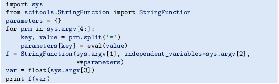
• b)

  

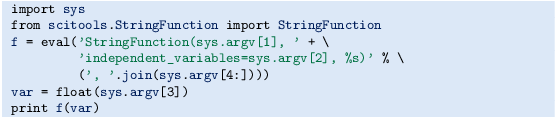
Filename: cml_functions.

Exercise 6.13 (Interpret function specifications)

To specify arbitrary functions $f(x_{1},x_{2},\ldots;p_{1},p_{2},\ldots)$ with independent variables $x_{1},x_{2},\ldots$ and a set of parameters $p_{1},p_{2},\ldots$, we allow the following syntax on the command line or in a file:

where <expression> denotes the function formula, <list1> is a comma-separated list of the independent variables, and <list2> is a comma-separated list of name=value parameters. The part with parameters <list2> is omitted if there are no parameters. The names of the independent variables and the parameters can be chosen freely as long as the names can be used as Python variables. Here are four different examples of what we can specify on the command line using this syntax:

Create a Python function that takes such function specifications as input and returns an appropriate StringFunction object. This object must be created from the function expression and the list of independent variables and parameters. For example, the last function specification above leads to the following StringFunction creation:

Write a test function for verifying the implementation (fill sys.argv with appropriate content prior to each individual test).

Hint

Use string operations to extract the various parts of the string. For example, the expression can be split out by calling split(’is a function of’). Typically, you need to extract <expression>, <list1>, and <list2>, and create a string like

and sending it to eval to create the object.

Filename: text2func.

Exercise 6.14 (Compare average temperatures in cities)

The tarfile src/misc/city_temp.tar.gzFootnote

http://tinyurl.com/pwyasaa/misc/city_temp.tar.gz

contains a set of files with temperature data for a large number of cities around the world. The files are in text format with four columns, containing the month number, the date, the year, and the temperature, respectively. Missing temperature observations are represented by the value −99. The mapping between the names of the text files and the names of the cities are defined in an HTML file citylistWorld.htm.

• a) Write a function that can read the citylistWorld.htm file and create a dictionary with mapping between city and filenames.

• b) Write a function that takes this dictionary and a city name as input, opens the corresponding text file, and loads the data into an appropriate data structure (dictionary of arrays and city name is a suggestion).

• c) Write a function that can take a number of data structures and the corresponding city names to create a plot of the temperatures over a certain time period.

Filename: temperature_data.

Exercise 6.15 (Generate an HTML report with figures)

The goal of this exercise is to let a program write a report in HTML format containing the solution to Exercise 5.14. First, include the program from that exercise, with additional explaining text if necessary. Program code can be placed inside <pre> and </pre> tags. Second, insert three plots of the $f(x,t)$ function for three different t values (find suitable t values that illustrate the displacement of the wave packet). Third, add an animated GIF file with the movie of $f(x,t)$. Insert headlines (<h1> tags) wherever appropriate.

Filename: wavepacket_report.

Exercise 6.16 (Allow different types for a function argument)

Consider the family of find_consensus_v* functions from Sect. 6.5.2. The different versions work on different representations of the frequency matrix. Make a unified find_consensus function that accepts different data structures for the frequency_matrix. Test on the type of data structure and perform the necessary actions.

Filename: find_consensus.

Exercise 6.17 (Make a function more robust)

Consider the function get_base_counts(dna) from Sect. 6.5.3, which counts how many times A, C, G, and T appears in the string dna:

Unfortunately, this function crashes if other letters appear in dna. Write an enhanced function get_base_counts2 which solves this problem. Test it on a string like ’ADLSTTLLD’.

Filename: get_base_counts2.

Exercise 6.18 (Find proportion of bases inside/outside exons)

Consider the lactase gene as described in Sects. 6.5.4 and 6.5.5. What is the proportion of base A inside and outside exons of the lactase gene?

Hint

Write a function get_exons, which returns all the substrings of the exon regions concatenated. Also write a function get_introns, which returns all the substrings between the exon regions concatenated. The function get_base_frequencies from Sect. 6.5.3 can then be used to analyze the frequencies of bases A, C, G, and T in the two strings.

Filename: prop_A_exons.