
Abstract
Cooperative advertising is an important mechanism used by manufacturers to influence retailers’ promotional decisions. In a typical arrangement, the manufacturer agrees to reimburse a fraction of a retailer’s advertising cost, known as the subsidy rate. We consider a case of new product adoption of a durable good with retail oligopoly, in which a manufacturer sells through a number of independent and competing retailers. We model the problem as a Stackelberg differential game with the manufacturer as the leader and the retailers as followers. The manufacturer announces his subsidy rates for the retailers, and the retailers in response play a Nash differential game to increase their cumulative sales and choose their optimal advertising efforts. We obtain feedback Stackelberg strategies consisting of manufacturer’s subsidy rates and retailers’ optimal advertising efforts. We obtain the conditions under which it is optimal for the manufacturer to not offer any advertising subsidy and study the role of retail competition on the manufacturer’s subsidy rates decisions. For a special case of two retailers, using a linear demand formulation, we present managerial insights on issues such as: dependence of subsidy rates on key model parameters, impact on channel profits and channel coordination, and finally, a case of an anti-discrimination legislation which restricts the manufacturer to offer equal subsidy rates to the two retailers.
Access provided by Autonomous University of Puebla. Download chapter PDF
Keywords
These keywords were added by machine and not by the authors. This process is experimental and the keywords may be updated as the learning algorithm improves.
1 Introduction
Firms spend huge sums of money in advertising, particularly in competitive markets. For some product categories, a firm’s market performance and competitiveness over its competitor relies heavily upon its advertising and promotional strategy. Quite often, the responsibility of local advertising lies with the retailers as they usually have much better knowledge about customers and local advertising channels such as TV stations, local newspapers, radio stations, etc. Since advertising can be quite expensive, a retailer might not advertise to the extent desired by the manufacturer, whose product the retailer is selling. In such a case, the manufacturer may consider providing some incentive to the retailer to advertise more. An important incentive comes in the form of cooperative advertising, an important and commonly used arrangement in which the manufacturer agrees to reimburse a fraction of the retailer’s advertising expenditures in selling his product (Bergen and John 1997). This fraction is commonly known as the ‘subsidy rate.’
Cooperative advertising is a fast growing activity amounting to billions of dollars a year, and it can be a significant portion of the advertising budgets of a manufacturer. Nagler (2006) found that the total expenditure on cooperative advertising in 2000 was estimated at $15 billion, compared with $900 million in 1970. Recent estimates put a figure of more than $25 billion for 2007. According to Dant and Berger (1996), as many as 25–40 % of local advertisements and promotions are cooperatively funded. In addition, Dutta et al. (1995) reported that the subsidy rates differ from industry to industry: it was 88.38 % for consumer convenience products, 69.85 % for other consumer products, and 69.29 % for industrial products.
Many researchers in the past have used static models to study cooperative advertising. Berger (1972) modeled cooperative advertising in the form of a wholesale price discount offered by a manufacturer to his retailer as an advertising allowance. He concluded that both the manufacturer and the retailer can do better with cooperative advertising. Dant and Berger (1996) extended the Berger model to incorporate demand uncertainty. Kali (1998) studied cooperative advertising from the perspective of coordinating a manufacturer-retailer channel. Huang et al. (2002) allowed for advertising by a manufacturer in addition to cooperative advertising. They also justified their static model by making a case for short-term effects of promotion.
Jørgensen et al. (2000) formulated a dynamic model with cooperative advertising as a Stackelberg differential game between a manufacturer and his retailer with the manufacturer as the leader. They considered short term as well as long term forms of advertising efforts made by the retailer as well as the manufacturer. They showed that the manufacturer’s support of both types of retail advertising benefits both channel members more than the support of only one type, and support of one type is better than no support at all. Jørgensen et al. (2001) modified the above model by introducing decreasing marginal returns to goodwill and studied two scenarios: a Nash game without advertising support and a Stackelberg game with support from the manufacturer as the leader. They characterized stationary feedback policies in both cases. Jørgensen et al. (2003) explored the possibility of advertising cooperation even when the retailer’s promotional efforts may erode the brand image. Karray and Zaccour (2005) extended the above model to consider both the manufacturer’s national advertising and the retailer’s local promotional effort. All of these papers use the Nerlove–Arrow (1962) model, in which goodwill increases linearly in advertising and decreases linearly in goodwill, and there is no interaction term between the sales and the advertising effort in the dynamics of sales. He et al. (2009) solved a manufacturer-retailer Stackelberg differential game with cooperative advertising using the Sethi (1983) model. He et al. (2011) considered a cooperative advertising channel consisting of a manufacturer selling its product through two retailers. In their study, they used a Lanchester-style extension of the Sethi model, in which the two competitors split the total market.
In this chapter, we study cooperative advertising in the case of durable goods. A durable good can be defined as a commodity which, once purchased by the consumer, does not need to be repurchased for a lengthy period of time. Examples of durable goods include cars, TV’s, microwave ovens, washing machines, etc. The market potential of such items depletes with time as cumulative sales increase and, eventually, saturation is reached. The advertising decisions for such products can be crucial, particularly in the early stages of their diffusion in the market. The modeling of durable goods sales dynamics is important in economics and management science. Many researchers in the past have studied the sales-advertising dynamics to study new product adoption for durable goods. Mahajan et al. (1990) review some of these models. A well known example of such a model is the Bass (1969) model of innovation diffusion, given by
where X(t) is the cumulative sales by time t, and a and b are positive constants. Many researchers have extended this model by highlighting the dependence of these constants on pricing and advertising policies. Feichtinger et al. (1994) reviewed such models. From the point of view of our research, we use the following model developed recently by Sethi et al. (2008):
where X(t) is the cumulative sales by time t with the total market potential normalized to one, D(p(t)) is the demand as a function of price p(t) with ∂D(p(t))/∂p(t)<0, u(t) is the advertising effort rate at time t, and ρ is the effectiveness of advertising. Krishnamoorthy et al. (2010) presented its duopolistic extension in which the sales-dynamics is given by
where the subscript i refers to firm i, i=1,2.
We study a dynamic cooperative advertising model for a retail market oligopoly of a durable product. We use an oligopolistic extension of (3), specified in the next section as our sales dynamics. The manufacturer sells his product through n independent and competing retailers and may choose to share their advertising costs. We model the problem as a Stackelberg differential game in which the manufacturer, as the leader announces his subsidy rates for the n retailers, and the retailers, acting as followers, respond by choosing their respective advertising efforts. The retailers, thus compete among themselves to increase their cumulative sales and play a Nash differential game to find their optimal advertising efforts.
To the best of our knowledge, with the exception of Chutani and Sethi (2012a), there has not been much work addressing the issue of manufacturer’s promotional support decisions for a dynamic market of durable goods. Chutani and Sethi (2012a) studied optimal pricing and advertising decisions for a retailer duopoly of durable goods. They considered the wholesale and retail prices, the retailers’ advertising efforts, and the manufacturer’s subsidy rates to the retailers’ advertising efforts as decision variables. They found that for a linear demand formulation, the manufacturer’s optimal subsidy rates are constant and independent of the model parameters. In this chapter, we study an oligopoly of n retailers with only the retailers’ advertising efforts and the manufacturer’s subsidy rates to those efforts as decision variables. By keeping the wholesale and retail prices as exogenously given, we can focus only on the advertising decisions. This allows us to obtain important managerial insights on such key issues as dependence of subsidy rates on various model parameters, threshold conditions for non-zero subsidy rates, channel coordination with optimal subsidy rates, and the impact of an anti-discrimination legislation when applied to subsidy rates.
In comparison to Chutani and Sethi (2012b) who also study cooperative advertising in a retailer oligopoly setting for a perishable goods market, we focus on durable goods such as refrigerators and vacuum cleaners. In our paper, the state variable is cumulative sales to account for the fact that those who have already purchased the good are no longer in the market, and its derivative, namely the sales rate, enters into the objective function. On the other hand, with frequently purchased goods such as soft drinks and soaps, the customers do not exit the market after their purchases, although they may switch to other brands for their future purchases. Thus in the perishable goods setting, the state is the rate of sales, expressed often times as a fraction of the market potential. It is this sales rate that enters directly into the objective function and makes the model of Chutani and Sethi (2012b) quite different from the model discussed in this chapter. There is another difference between the two models, i.e., the absence of the decay term in (3). This is due to the fact that the cumulative sales, which have already taken place, do not decay. In the perishable goods case, on the other hand, the decay term is ascribed to the effect of factors such as competition, product obsolescence, forgetting, etc., on the change in the rate of sales.
Thus, we make contributions to the existing literature in areas of cooperative advertising, durable goods sales-advertising dynamics, and supply chain coordination by answering the following key research questions. First, what are the optimal subsidy rates of the manufacturer and the optimal advertising responses by the retailers in feedback form for a durable goods retail oligopoly? Second, is cooperative advertising always optimal for the manufacturer, or are there cases under which it is optimal for the manufacturer not to offer any subsidy to the retailers? Moreover, whenever possible, we find a threshold condition, based on model parameters, which delineates the cases under which no subsidy is optimal for the manufacturer. Third, what role does retail level competition play on the subsidy rate policies? Fourth, how do subsidy rates depend on various model parameters? Fifth, what is the impact of a coop advertising program on the profits of all the members in the channel? How does the channel profit with coop program compare to that without coop advertising, and to the integrated channel profit? Can coop advertising lead to better channel coordination? Finally, sixth, what are the effects of an anti-discrimination legislation that restricts the manufacturer to offer equal subsidy rates to his retailers. How does it impact the optimal subsidy rates, profits of all the members in the channel, and the total channel profit?
The rest of the chapter is organized as follows. In Sect. 2 we describe the model in detail, followed by some preliminary results in Sect. 3. In Sect. 4, we consider a special case of identical retailers and obtain some explicit analytical results along with some useful insights. In Sect. 5, we study a special case of two competing retailers. We perform numerical analysis in a general case and examine the effect of various model parameters on the optimal subsidy rates in the special case of linear demand. In the same section, we discuss the issue of channel coordination with cooperative advertising. In this special case of two retailers, we discuss an extension in which the manufacturer is required to offer equal subsidy rates, if any, to both the retailers. We also study the impact of such an anti-discriminatory act on the profits of all the channel members and on the performance of the channel as a whole. Finally, we conclude the chapter and summarize our findings in Sect. 6.
2 The Model
We consider a model in which a manufacturer sells his product through n independent and competing retailers, labeled 1,2,…,n. The manufacturer may subsidize the advertising expenditures of the retailers. The subsidy, expressed as a fraction of a retailer’s total advertising expenditure, is referred to as the manufacturer’s subsidy rate to that retailer. We now introduce key notation used in the chapter:
- t :
-
Time t∈[0,∞),
- i :
-
Indicates retailer i, i=1,2,…,n, when used as a subscript,
- X i (t)∈[0,1]:
-
Cumulative normalized sales of retailer i,
- \(\bar{X}(t)= \sum_{j=1}^{N}{X_{i}(t)}\) :
-
Total cumulative sales combined over n retailers,
- X(t)≡(X 1(t),X 2(t),…,X n (t)):
-
Cumulative sales vector of n retailers at time t,
- u i (t):
-
Retailer i’s advertising effort rate at time t,
- w i :
-
Wholesale price for retailer i,
- p i :
-
Retail price of retailer i,
- p i −w i =m i :
-
Margin of retailer i,
- θ i (t)≥0:
-
Manufacturer’s subsidy rate for retailer i at time t,
- Θ(X(t))≡(θ 1(X(t)),…,θ n (X(t))):
-
Subsidy rate vector in feedback form at time t,
- D i :
-
Demand of goods sold by retailer i, D i ≥0,
- ρ i >0:
-
Advertising effectiveness parameter of retailer i,
- r>0:
-
Discount rate of the manufacturer and the retailers,
- V i , V m :
-
Value functions of retailer i and of the manufacturer, respectively,
- V I :
-
Value function of the integrated channel.
Without any loss of generality, we assume that the manufacturing cost of the product is zero. Thus, the margin for the manufacturer from retailer i is equal to the wholesale price w i . Furthermore, we use the standard notations, i.e., \(V_{iX_{j}} = \partial V_{i}/\partial X_{j}\), i=1,2,…,n, j=1,2,…,n, and \(V_{mX_{i}} = \partial V_{m}/\partial X_{i}\) and \(V_{X_{i}} = \partial V/\partial X_{i}\), i=1,2,…,n. For simplicity, X(t) and Θ(X(t)) are also referred to as X, and Θ(X), respectively
We normalize the total market potential to be one and the cumulative normalized sales of the retailer i, at time t to be denoted by X i (t), i=1,2,…,n. The rate of change of cumulative units sold, which is the instantaneous rate of sales, is denoted by \(\dot{X_{i}}(t)\), and is given by
where \(\bar{X}(t) = \sum_{j=1}^{n}X_{j}(t)\) is the cumulative sales of the manufacturer at time t, u i (t) is the retailer i’s advertising effort at time t, ρ i is the effectiveness of firm i’s advertising, and D i is the demand of retailer i. The state of the system is denoted by the cumulative sales vector, i.e., X(t)≡{X i (t)}=(X 1(t),X 2(t),…,X n (t)). The sequence of events is shown in Fig. 1. The manufacturer as the Stackelberg leader announces the subsidy rate θ i (t) for retailer i, i=1,2,…,n, at time t. The retailers, acting as followers respond by choosing their respective advertising efforts u i (t), i=1,2,…,n, by playing a Nash differential game to increase their sales.

Sequence of events
For a solution of our game, we adopt the concept of a feedback Stackelberg equilibrium (see, e.g., Başar and Olsder 1999, and Bensoussan et al. 2014). This type of equilibrium is subgame perfect as well as strongly time-consistent (see Başar and Olsder 1999). Accordingly, the manufacturer’s subsidy rates policy, denoted by its subsidy rate vector Θ(X)≡(θ 1(X),θ 2(X),…,θ n (X)), is expressed as a function of the cumulative sales vector X≡(X 1,X 2,…,X n ). Thus, the subsidy rates at time t≥0 are θ i (X(t)), i=1,2,…,n. The retailers in response choose their optimal advertising efforts by solving their respective optimization problems. The cost of advertising is quadratic in the advertising effort, representing a marginal diminishing effect of advertising. The use of such quadratic cost function is common in the literature. Retailer i’s optimal control problem is to maximize the present value of his profit stream over the infinite horizon, i.e.,
subject to (4), where p i −w i =m i equals the margin of retailer i and V i (X) is referred to as the value function of retailer i. The vector X=(X 1,X 2,…,X n ) is the vector of initial conditions such that X i ≥0, ∀i=1,2,…,n and \(\sum_{i=1}^{n} X_{i} \leq1\). The solution to the Nash differential game defined by (4)–(5) gives retailer i’s feedback advertising effort u i (X(t)), i=1,2,…,n, which, with a slight abuse of notation, can be written as u i (X 1,X 2,…,X n ∣θ 1(X 1,X 2,…,X n ),…,θ n (X 1,X 2,…,X n ))≡u i (X∣θ(X)), i=1,2,…,n.
The manufacturer anticipates the retailers’ optimal responses and incorporates them into his optimization problem, which is a stationary infinite horizon optimal control problem:
subject to for i=1,2,…,n
The solution to the optimal control problem (6)–(7) gives the optimal subsidy policy in feedback form, which is expressed as \(\theta^{*}_{i}(X_{1}, X_{2}, \ldots, X_{n}) \equiv\theta^{*}_{i}(X)\). We can also write retailer i’s feedback advertising policy, with a slight abuse of notation, as \(u^{*}_{i}(X) \equiv u^{*}_{i}(X \mid\theta^{*}_{1}(X), \ldots, \theta^{*}_{n}(X)) \equiv u^{*}_{i}(X \mid\varTheta^{*}(X))\), i=1,2,…,n.
The subsidy rate and advertising policies, \(\theta^{*}_{i}(X)\) and \(u^{*}_{i}(X)\), i=1,2,…,n, respectively, constitute a feedback Stackelberg equilibrium of the problem (4)–(7). Substituting these policies into the state equations (4) gives the cumulative sales vector \(X^{*}(t) = (X^{*}_{1}(t), X^{*}_{2}(t), \ldots, X^{*}_{n}(t))\), t≥0, and the decisions of the manufacturer and the retailers, as \(\theta^{*}_{i} = \theta^{*}_{i}(t) = \theta^{*}_{i}(X(t))\) and \(u^{*}_{i} = u^{*}_{i}(t) = u^{*}_{i}(X^{*}(t))\), i=1,2,…,n, t≥0, respectively.
3 Preliminary Results
We first solve retailer i’s problem to find the optimal advertising policy \(u^{*}_{i}(X\mid\varTheta(X))\), given the subsidy rates θ i (X), i=1,2,…,n, announced by the manufacturer. The Hamilton–Jacobi–Bellman (HJB) equation for the value function of retailer i, i=1,2,…,n, is
where \(V_{iX_{j}}\) represents the marginal increase in the total discounted profit of retailer i, i=1,2,…,n, with respect to an increase in the cumulative sales of retailer j, j=1,2,…,n.
Remark 1
Although we have restricted θ i (X), i=1,2,…,n, to be nonnegative, it is obvious that 0≤θ i (X)<1, i=1,2,…,n. This is because, if the optimal subsidy rate for a retailer were greater than or equal to one, then that retailer would choose to have an infinite level of advertising, resulting in the manufacturer’s value function to be −∞. This would mean that the manufacturer would have even less profit than he would have by not subsidizing any retailer at all. Since the manufacturer is the leader, it also follows that optimal subsidy rates are less than one.
We now obtain the optimal advertising policy of a retailer i, given the subsidy rate policy of the manufacturer.
Proposition 1
For a given subsidy rate policy θ i (X), i=1,2,…,n, the optimal feedback advertising decision of retailer i is
and the value function V i (X) satisfies the partial differential equation
Proof
Using the first-order conditions w.r.t. u i in (8), i=1,2,…,n, we obtain (9), and then use (9) in (8) to obtain (10). The second order conditions are also satisfied as it can be seen that V i (X) is concave in u i . □
We can see that the advertising effort by retailer i increases with his demand D i and with the marginal benefit of his own market share. Moreover, the advertising effort is greater for a higher un-captured market (\(1-\bar{X}\)). Taking into account retailers’ optimal responses to his subsidy rates policy, the manufacturer solves his problem to obtain his optimal subsidy rates. The HJB equation for the manufacturer’s value function V m (X) is
Using (9), we can rewrite the above HJB equation as
We can now obtain the manufacturer’s optimal subsidy rates policy as shown below.
Proposition 2
The manufacturer’s optimal subsidy rate for retailer i is
where
and the manufacturer’s value function V m (X) satisfies
Proof
The first-order conditions w.r.t. θ i , i=1,2,…,n, in (11) give a unique solution, i.e., \(\hat{\theta}_{i}\), i=1,2,…,n, as shown in (13). This along with Remark 1 yields the optimal subsidy rates policy as in (12). Finally, we obtain (14) by using (12) in (11). In order to verify the second-order conditions for the optimality of the subsidy rates, we compute the Hessian matrix \(\frac{\partial^{2} V_{m}(X)}{\partial\theta_{i} \partial \theta_{j}}\), i=1,2,…,n, j=1,2,…,n. We find that \(\frac{\partial^{2} V_{m}(X)}{ \partial\theta_{i} \partial\theta_{j}} = 0\) for i≠j, and \(\frac {\partial^{2} V_{m}(X)}{ \partial\theta^{2}_{i}} < 0\) when we use \(\theta_{i} = \hat{\theta}_{i}\), i=1,2,…,n. Therefore, the Hessian matrix is negative definite for \(\theta_{i} = \hat{\theta}_{i}\), ∀i=1,2,…,n, and the second-order conditions are satisfied. □
Equation (13) shows that the optimal subsidy rate offered by the manufacturer to retailer i increases as the manufacturer’s marginal profit with respect to the cumulative sales of retailer i increases. Thus, the manufacturer provides more support to the retailer who offers a higher marginal profit from his sales to the manufacturer. However, as a retailer’s own marginal profit with respect to his cumulative sales increases, then the subsidy rate offered by the manufacturer to that retailer decreases. This is because the manufacturer is aware that the retailer has his own incentive to increase his sales by advertising more, and so the manufacturer would lower his subsidy rate to that retailer. Moreover, by using (13) in (9), we see that \(u^{*}_{i}(X) = \frac{1}{4} (\rho _{i}D_{i}(p_{i})(2(w_{i}+V_{mX_{i}})+(p_{i}-w_{i}+V_{iX_{i}}))\sqrt{1-\bar{X}} )\), which shows that the advertising effort by retailer i increases with the marginal profit of the retailer as well as that of the manufacturer with respect to his cumulative sales.
To obtain the optimal advertising and subsidy rate strategies which constitute a feedback Stackelberg equilibrium, we must find continuously differentiable functions V i (X), i=1,2,…,n, and V m (X) that satisfy equations (10) and (14), respectively. As in Sethi et al. (2008), we look for affine value functions
where α and β i , i=1,2,…,n, are constants, and later show that these solve (10) and (14). In order to obtain the coefficients α and β i , i=1,2,…,n, we see from (15) and (16) that
We can also see that with (15)–(16), \(\hat{\theta _{i}}(X)\) and \(\theta^{*}_{i}(X)\), i=1,2,…,n, given in (12) and (13) will be constants, and thus, can be simply denoted as \(\hat{\theta_{i}}\) and \(\theta^{*}_{i}\), respectively, i=1,2,…,n.
We compare the coefficients of X i , i=1,2,…,n, and the constant term of the value functions V i (X), and V m (X) in equations (10), (14), and (15)–(16), and obtain the following nonlinear system of equations to be solved for the coefficients α and β i , i=1,2,…,n:
Using (17) and (20), we can obtain a condition under which the manufacturer will support retailer i. We define
The optimal subsidy rate for retailer i will clearly depend on the sign of P i , i=1,2,…,n. Thus, when P i >0, the manufacturer supports retailer i, otherwise he does not. When P i ≤0, ∀i, no retailer gets advertising support from the manufacturer. In this case, \(\theta^{*}_{i} = 0\), i=1,2,…,n, and the set of equations given by (18) can be solved independently of (19) for the coefficients β i , i=1,2,…,n. By computing the coefficients α and β i , i=1,2,…,n, when \(\theta^{*}_{i} = 0\), i=1,2,…,n, we can write the conditions for a zero subsidy rate for each retailer, i.e., P i ≤0, i=1,2,…,n, in terms of the model parameters p i , w i , ρ i and D i , i=1,2,…,n.
In general, it is difficult to obtain an explicit solution of the system of equations (18)–(20). However, in the special case of identical retailers, defined by m 1=m 2=⋯=m n (i.e., p 1−w 1=p 2−w 2=⋯=p n −w n ), D 1=D 2=⋯=D n , and ρ 1=ρ 2=⋯=ρ n , we can obtain some explicit results, including the values of P i , i=1,2,…,n. In addition to this, when M 1=M 2=⋯=M n i.e., w 1=w 2=⋯=w n ), more explicit results can be obtained. In the general case, nevertheless, it is easy to solve the system numerically and study the dependence of the subsidy rates on the various model parameters. We now consider some special cases to get some insights into the problem.
4 Special Case: n Identical Retailers
Let m i =p i −w i =m, D i =D, and ρ i =ρ, i=1,2,…,n. Without loss of generality, we can assume that w 1>w 2>w 3>⋯>w n−1>w n , which is equivalent to p 1<p 2<⋯<p n . In order to obtain the condition under which none of the retailers will be supported (i.e., P i ≤0, i=1,2,…,n), we set \(\theta^{*}_{i} = 0\), i=1,2,…,n, in equations (18)–(19) and then solve for β i , i=1,2,…,n, and α in an explicit form to obtain P i , i=1,2,…,n, as follows:
where \(W_{-i} = \sum_{^{j=1}_{j\neq i}}^{n}{w_{j}}\). The derivation of (22) is shown in the Appendix. We can now conclude the following result.
Proposition 3
When P i ≤0, i=1,2,…,n, we have a non-cooperative equilibrium in which it is optimal for the manufacturer not to support any retailer. Furthermore, if P i >0 and P j ≤0, j=1,2,…,n, j≠i, we have \(\theta ^{*}_{i} > 0\) and \(\theta^{*}_{j} = 0\), j=1,2,…,n, j≠i, that is, the manufacturer supports retailer i only.
We can observe that P i is linear in w j , i=1,2,…,n, j=1,2,…,n. In P i , the coefficient of w i is positive and that of w j , j≠i is negative. Thus, P i increases as the margin of the manufacturer from retailer i (which is the same as the wholesale price charged from retailer i) increases, and it decreases as the margin from any other retailers decreases. As retailer i pays a higher wholesale price to the manufacturer, his likelihood of receiving advertising support from the manufacturer increases. Moreover, this increase in w i further hampers the case of retailer j, j≠i, in getting support from the manufacturer. This is intuitive because it is beneficial for the manufacturer to support the retailer who is more profitable to him and increase his sales, and since the n retailers compete for the same market, it comes at a cost for the other n−1 retailers. Indeed, it can be seen that
which means that w i >w j implies P i >P j . Thus, when P i ≤0 and P j ≤0 for i≠j, retailer i will be the first to start receiving a positive subsidy rate, whenever changes in the parameters (m, D, ρ) cause the sign of P i to change from negative to positive, and retailer j will never receive any support as long as w i >w j . In other words, a retailer who pays a higher wholesale price is more likely to get a positive subsidy rate from the manufacturer when compared to a retailer who offers a lower wholesale price.
To further enhance the understanding of our results, we assume that the discount rate is very small, i.e., r≈0. Under this condition, the expressions for P i can be simplified to
where \(W_{-i} = \sum_{^{j=1}_{j\neq i}}^{n}{w_{j}}\). Equation (24) yields some useful insights from our analysis of the case of identical retailers for small values of the discount rate. We can see from (24) that if w i is less than the average wholesale price of other n−1 retailers, i.e., \(\frac {W_{-i}}{(n-1)}\), then retailer i will not be supported. In addition, if the retailers are also symmetric (i.e., w 1=w 2=⋯=w n ), then P i <0, i=1,2,…,n, and no retailer will be supported. If we assume that w j =0, j=2,3,…,n, j≠1, so that only retailer 1 sells the manufacturer’s product and all other retailers compete with retailer 1, then, under competition, the condition for support for retailer 1 is \(w_{1}\frac{(n-1)}{n} \geq m\frac{(n-1)}{(2n-1)} = (p_{1}-w_{1})\frac {(n-1)}{(2n-1)}\). Furthermore, if the number of retailers n is very large, then retailer i receives advertising support when w i >m/2=(p i −w i )/2, i.e. when the manufacturer’s margin from retailer i is at-least half of retailer i’s margin.
5 Special Case: Two Non-identical Retailers
In this section, we further explore our model in the case of two non-identical retailers, to get some useful managerial insights. We look into issues such as dependence of subsidy rates on different model parameters, issue of channel coordination and profits of the channel members with cooperative advertising, and a case of anti-discriminatory legislation.
5.1 Numerical Analysis
We perform numerical analysis to study the dependence of the manufacturer’s subsidy rates on wholesale prices (w 1,w 2), retailers’ margins (p 1−w 1,p 2−w 2), and advertising effectiveness coefficients (ρ 1,ρ 2). We consider a linear demand form and study the impact of the price sensitivity of demand on the subsidy rates. In this analysis, we first take a base case with a value for each parameter and then vary different parameters one by one to study their impacts on \(\theta^{*}_{1}\) and \(\theta^{*}_{2}\). To study the effect of retailer 1’s margin, we vary p 1 and keep all other parameters unchanged. Similarly, by changing w 1 and keeping all other parameters constant, we study the impact of manufacturer’s margin. We consider the following demand specification for given retail prices:
where η i represents the price sensitivity of the demand. The linear demand function is popular in the literature (e.g., Petruzzi and Dada 1999; Sethi et al. 2008; Krishnamoorthy et al. 2010). We perform numerical analysis for a wide range of parameters and present some representative results for a base case of w 1=w 2=0.3, p 1=p 2=0.6, η 1=η 2=1, and ρ 1=ρ 2=1. Thus in the base case m 1=m 2=0.3.
-
(a)
Effect of the manufacturer’s margin Fig. 2: We vary w 1 to change the manufacturer’s margin from retailer 1, but also change p 1 accordingly to keep retailer 1’s margin (p 1−w 1) constant. Note that as p 1 increases retailer 1’s demand D 1 decreases. We find that as w 1 increases, the manufacturer starts offering a higher subsidy rate to retailer 1, rewarding him for providing a higher margin. Retailer 2’s subsidy rate decreases initially and then increases. The retailer who offers a higher margin (wholesale price) to the manufacturer gets a higher subsidy rate.
Fig. 2 
Subsidy rates vs. w 1, fixed p 1−w 1
-
(b)
Effect of the manufacturer’s margin and changing retailer 1’s margin Fig. 3: We vary w 1 to change the manufacturer’s margin and keep p 1 constant, thereby changing retailer 1’s margin as well. As w 1 increases, the manufacturer offers a higher subsidy rate to retailer 1 and reduces the subsidy rate to retailer 2. Since p 1 remains constant, retailer 1’s margin decreases as w 1 increases, so he has less incentive to advertise. The manufacturer rewards retailer 1, now that he gives him a higher margin, by increasing his subsidy rate, and simultaneously reduces the subsidy rate of retailer 2. The manufacturer gives a higher subsidy rate to the retailer who gives a higher margin.
Fig. 3 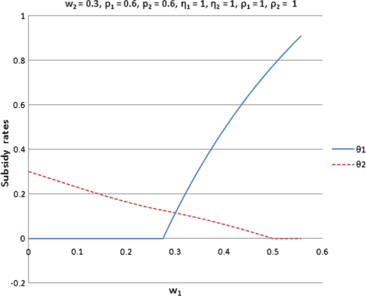
Subsidy rates vs. w 1
-
(c)
Effect of retail price (and hence retailer’s margin) Fig. 4: As p 1 increases, retailer 1’s margin increases and demand D 1 decreases. With a higher p 1, the manufacturer knows that retailer 1 has a higher incentive of his own to advertise more. Moreover as retailer 1’s demand decreases, the manufacturer sees a greater possibility of increase in its sales through retailer 2. The combined effect of these factors makes the subsidy rate for retailer 1 to decrease and that of retailer 2 to increase gradually. The retailer with the lower retail price gets a higher subsidy rate.
Fig. 4 
Subsidy rates vs. p 1
-
(d)
Effect of the advertising effectiveness parameter Fig. 5: As the advertising effectiveness of retailer 1 increases, the subsidy rates for both retailers decrease. The rate of decrease is higher for retailer 2 than for retailer 1. All other parameters being the same, the retailer with the higher advertising effectiveness gets a higher subsidy rate.
Fig. 5 
Subsidy rates vs. ρ 1
-
(e)
Effect of the price sensitivity of demand Fig. 6: As η 1 increases, D 1=1−η 1 p 1 decreases. The manufacturer increases the subsidy rate for both retailers. The retailer with the higher price sensitivity gets a lower subsidy rate.
Fig. 6 
Subsidy rates vs. η 1


5.2 Channel Coordination
In this section, we analyze the impact of cooperative advertising arrangement on the profits of the manufacturer and the retailers, and thereby investigate the role of cooperative advertising in coordinating the channel and improving the overall channel profit. We compare the value functions of the channel members and that of the channel as a whole in three cases: (i) an integrated channel in which the advertising decisions are taken on the basis of maximization of the total combined profit of the manufacturer and the retailers, (ii) a decentralized channel with optimal subsidy rates, where the manufacturer chooses the optimal subsidy rates and the retailers decide their optimal levels of advertising, and (iii) a decentralized channel without any cooperative advertising.
In the integrated channel case, the optimization problem to decide the optimal level of advertising can be written as follows:
subject to
The HJB equation for the integrated channel value function V I is
where \(\dot{X_{1}}\) and \(\dot{X_{2}}\) are given by (27). Using (27) in the HJB equation (28) and applying the first-order conditions for maximization with respect to u 1 and u 2, we obtain the following
Proposition 4
The optimal feedback advertising policies for the integrated channel are
and the value function of the integrated channel satisfies the partial differential equation
Proof
We obtain (29) by applying the first-order conditions with respect to u 1 and u 2 in the HJB equation (28), and (30) can be obtained by using (29) and (27) in (28). □
Once again, we show that
solves (30), for some α I to be determined. Since \(\alpha^{I} = -V^{I}_{X_{1}} = -V^{I}_{X_{2}}\) is a constant, it must satisfy the equation
This is a quadratic equation in α I which gives two real roots. We choose the one which gives p 1−α I≥0 and p 2−α I≥0, as it ensures \(u^{*}_{1} \geq0\) and \(u^{*}_{2} \geq0\). We therefore have
In the second case, we consider a decentralized channel with cooperative advertising, where the manufacturer chooses the optimal subsidy rates. We define the value function in this case as \(V^{c}(X_{1}, X_{2}) = V^{c}_{m}(X_{1}, X_{2}) + V^{c}_{r}(X_{1}, X_{2})\), where \(V^{c}_{m}\) is the manufacturer’s value function (given by (16)) and \(V^{c}_{r}\) is the sum of the value functions of the two retailers obtained by (15).
The third case is of a decentralized channel with no cooperation, with the channel value function defined as \(V^{n}(X_{1}, X_{2}) = V^{n}_{m}(X_{1}, X_{2}) + V^{n}_{r}(X_{1}, X_{2})\), where \(V^{n}_{m}\) and \(V^{n}_{r}\) are the manufacturer’s value function and the sum of the two retailers’ value functions, respectively, in the non-cooperative setting. These value functions are computed by setting \(\theta^{*}_{1} = \theta ^{*}_{2} = 0\) in (18)–(19), and then using the resulting values of α, β 1, and β 2 in (15)–(16). We term the values of these coefficients in the non-cooperative case as α n, \(\beta^{n}_{1}\), and \(\beta ^{n}_{2}\), respectively.
Since the manufacturer is the leader and decides the subsidy rates by maximizing his total discounted profit, it is obvious that
In general, it is difficult to establish explicit analytical relationships between the value functions of the retailers and the channel as a whole. We therefore use numerical analysis to study the effect of cooperative advertising on the profits of all the parties in the channel. Recall that V I=α I(1−X 1−X 2), V c=(α+β 1+β 2)(1−X 1−X 2), and \(V^{n} = (\alpha^{n}+\beta^{n}_{1}+\beta^{n}_{2})(1-X_{1}-X_{2})\). Thus, in order to do a comparison of any two value functions, it is sufficient to compare their respective coefficients of (1−X 1−X 2). We study V I, V c and V n with respect to the changes in the optimal subsidy rates brought about by changes in the model parameters. In the results shown, the changes in the value functions correspond to the changes in the margin of retailer 1 (caused by changes in p 1). As p 1 increases, we know from Fig. 4 that θ 1 decreases, and θ 2 increases gradually. Figure 7 depicts the values of α I, (α+β 1+β 2), and \((\alpha^{n}+\beta^{n}_{1}+\beta^{n}_{2})\), and thus compares V I, V c, and V n, respectively, for D 1=1−η 1 p 1, D 2=1−η 2 p 2, p 2=0.6, w 1=0.3, w 2=0.3, η 1=1, η 2=1, ρ 1=1, and ρ 2=1. Thus, for any point in Fig. 7, the values of the optimal subsidy rates are the same as the corresponding values in Fig. 4. We find that under all instances, \(\alpha^{I} > (\alpha+\beta_{1}+\beta_{2}) > (\alpha^{n}+\beta ^{n}_{1}+\beta^{n}_{2})\), and thus V I>V c>V n. The result that V I is the highest of all is obvious, as we expect the integrated channel value function to be greater than that in the decentralized channel, with or without cooperative advertising. This result also indicates that through a cooperative advertising mechanism, as proposed in our model, total channel profit can be increased and better channel coordination can be achieved. The level of partial coordination measured by the ratio (V c−V n)/(V I−V n) is found to be as high as 82.5 %.

Channel value functions in integrated, coop, and non-cooperative cases
Figure 8 shows the difference in the value function coefficients between cooperative and non-cooperative settings for the manufacturer, the two retailers, and the total channel, i.e., α−α n, \(\beta_{1}-\beta^{n}_{1}\), \(\beta_{2}-\beta^{n}_{2}\), and \((\alpha+\beta_{1}+\beta_{2})-(\alpha^{n}+\beta^{n}_{1}+\beta^{n}_{2})\), respectively. Once again, we use D 1=1−η 1 p 1, D 2=1−η 2 p 2, p 2=0.6, w 1=0.3, w 2=0.3, η 1=1, η 2=1, ρ 1=1, and ρ 2=1. As expected, the manufacturer always benefits from cooperative advertising. In view of results in Fig. 4, we can see that the manufacturer’s benefit is higher when, roughly speaking, the difference between the subsidy rates of the two retailers is higher. The retailers, however, do not seem to benefit always from cooperative advertising. It is found that when a retailer receives a much lower subsidy rate in comparison to his competitor, he does not seem to benefit from this arrangement. In other words, when \(\theta^{*}_{1}-\theta^{*}_{2}\) is high, retailer 2 does not benefit from cooperative advertising, and vice versa. Figure 8 also shows that the region in which both retailers benefit from cooperative advertising is a small range of values of p 1, around the point when p 1=p 2, which is when both retailers receive almost equal subsidy rates. Thus, the retailer which has a higher margin relative to his competitor and thus gets a significantly lower subsidy rate from the manufacturer, might not prefer a cooperative advertising arrangement.

Difference between the value functions in the coop case and the non-coop case
These observations raise the issue of the manufacturer preferring one retailer over the other, in terms of subsidy rates, particularly when it seems that the retailer receiving a significantly lower subsidy rate might make less profit from cooperative advertising than without it. Next, we study the effect of an anti-discriminatory legislation, such as the Robinson–Patman Act of 1936, which would compel the manufacturer to offer equal subsidy rates to both retailers.
5.3 Equal Subsidy Rate for Both Retailers
We consider the case when the manufacturer is required to offer equal subsidy rates to both retailers. We let \(V^{RP}_{m}(X_{1}, X_{2})\), \(V^{RP}_{1}(X_{1}, X_{2})\), \(V^{RP}_{2}(X_{1}, X_{2})\), and V RP(X 1,X 2) denote the value functions of the manufacturer, retailer 1, retailer 2, and the total channel, respectively, with the superscript RP standing for Robinson and Patman. These value functions solve the control problems defined by (4)–(6) with θ 1=θ 2=θ, as the manufacturer’s optimization problem now has only one subsidy rate decision. As in the general model, we obtain value functions that are linear in X 1 and X 2 and are a multiple of (1−X 1−X 2), and we express them as in (15)–(16). The value function coefficients for the manufacturer and the two retailers are now defined as α rp, \(\beta^{rp}_{1}\), and \(\beta ^{rp}_{2}\), respectively. The coefficients solve the system of equations obtained by setting \(\theta^{*}_{1} = \theta^{*}_{2} = \theta^{*}\) in (18)–(19). We thus have the following system of equations:
where
The threshold for no cooperation with both retailers is that
We perform numerical analysis to study the behavior of θ ∗ with respect to different model parameters and compare it with the optimal subsidy rates in the general model with no restriction on the subsidy rates. Figures 9, 10, 11, 12, and 13 show the dependence of θ ∗ on w 1 with fixed p 1−w 1, w 1 with fixed p 1, p 1, ρ 1, and η 1, respectively, and compare θ ∗ with \(\theta ^{*}_{1}\) and \(\theta^{*}_{2}\) (optimal subsidy rates with no legislation in effect) for linear demand, i.e., D i =1−η i p i . We find that as w 1 and p 1 increase while keeping retailer 1’s margin (p 1−w 1) constant, the common subsidy rate for the two retailers increases, but at a decreasing rate Fig. 9. However, when the increase in w 1 is accompanied by a fixed p 1, thereby reducing retailer 1’s margin, we find that the common subsidy rate first increases and then decreases. As p 1 increases, θ ∗ changes in a more complicated decreasing-increasing fashion as shown in Fig. 11. Recall that an increase in p 1 causes D 1 to decrease. The dependence of the common subsidy rate on ρ 1 and η 1 is similar to the dependence of the optimal subsidy rates in the unrestricted model, i.e., decreasing with ρ 1 and increasing with η 1, as shown in Fig. 12, and Fig. 13.

Subsidy rate vs. w 1, constant p 1−w 1

Subsidy rate vs. w 1, constant p 1

Subsidy rate vs. p 1

Subsidy rate vs. ρ 1

Subsidy rate vs. η 1
We now investigate the impact of an anti-discriminatory legislation on the value functions of all the parties in the supply chain and on the channel value function. We compare the value functions in three cases: a channel without any cooperative advertising, a channel with no anti-discriminatory act and optimal subsidy rates, and a channel with an anti-discriminatory act and optimal common subsidy rate for both retailers. Recall that the value functions in our model take the form of a constant times (1−X 1−X 2), and thus we compare the value of these coefficients (α, β 1, β 2, α rp, \(\beta ^{rp}_{1}\), \(\beta^{rp}_{2}\), α n, \(\beta^{n}_{1}\), \(\beta^{n}_{2}\)) via numerical analysis to understand the comparison between the various value functions. Figures 14 and 15 show a comparison of these coefficients with changes in p 1. The values of the parameters are chosen so that for any point in these curves, the optimal subsidy rates (\(\theta^{*}_{1}\), \(\theta^{*}_{2}\), θ ∗) are the same as the corresponding values in Fig. 11. Figure 14 shows the impact of a Robinson–Patman like legislation on the profits of all the parties in the channel by plotting the difference between the value function coefficients with and without the legislation. As is obvious, the manufacturer does not benefit from this legislation because of the additional constraint on his optimization problem. The manufacturer’s loss is high when p 1 is very low, i.e., when the difference \(\theta^{*}_{1} - \theta^{*}_{2}\) is high. The manufacturer’s loss is low when the difference between the two optimal subsidy rates in the unconstrained problem is low. We find that the retailer receiving a higher subsidy rate in the absence of the legislation, does not benefit either. However, a less efficient retailer who would have received a lower subsidy rate without the legislation, benefits as his subsidy rate is increased under the act. Thus, when p 1 is low, retailer 1 loses and retailer 2 benefits, and when p 1 is high, retailer 1 loses and retailer 2 benefits from the legislation. Noticeably though, in all the instances studied, the gain of one retailer was not able to offset the losses of the other two parties and the total channel suffered as a whole. These results indicate that an anti-discriminatory legislation in the context of cooperative advertising could be beneficial to only one of the two retailers and not to the other parties, and could also result in a lower channel profit.

Impact of anti-discriminatory legislation on the value functions

Value functions in different cases divided by the integrated channel value function
Figure 15 compares the total profit of an integrated channel (V I) with the total channel profit in three cases: no advertising cooperation (V n), cooperation with no legislation (V c), and cooperation with equal subsidy rates (V rp), with a view of comparing the level of channel coordination possible in these three scenarios. Here again, we see that while an unrestricted cooperative advertising arrangement can coordinate the channel to a great extent (up to 85 %, as found previously), the enforcement of an anti-discriminatory law on the manufacturer can decrease the channel profit and thereby reduce the level of coordination achieved. The case of no advertising cooperation seems to perform worst of all with the lowest channel profit and thus, the lowest level of coordination. Once again, these results suggest that for a durable goods duopoly with a sales dynamics as ours, cooperative advertising with no regulation might be the best alternative of the three from the perspective of total channel profit.
6 Concluding Remarks
We study a cooperative advertising model for durable goods in a retail oligopoly of n independent and competing retailers. We obtain the Stackelberg equilibrium and obtain the optimal subsidy rates policy of the manufacturer and the optimal advertising policy of the retailers in feedback form. We explore the conditions under which it is not optimal for manufacturer to support retailers and compute this explicitly as a function of the model parameters in a special case of n identical retailers, and obtain managerial insights on the role of retail competition. For a special case of two non-identical retailers with linear demand, we numerically study the dependence of the optimal subsidy rate on the model parameters. We investigate the impact of cooperative advertising on the profits of the channel members in a channel with two retailers and explore the extent to which cooperative advertising can coordinate the channel. Our numerical analysis shows that a cooperative advertising arrangement can result in higher channel profit and greater supply chain coordination. However, we find that while the manufacturer always benefits with an arrangement with the optimal subsidy rates, the two retailers may not benefit simultaneously. Indeed, we find that both retailers seem to benefit when the retailer are nearly symmetric and thus the subsidy rates they receive are nearly equal. And finally, we consider a case of anti-discrimination legislation in the case of two retailers, in which the manufacturer is required to offer equal subsidy rates to the two retailers. We find that such a legislation may result in a lower channel coordination.
References
Başar, T., & Olsder, G. J. (1999). SIAM series in classics in applied mathematics. Dynamic noncooperative game theory. Philadelphia: Society for Industrial and Applied Mathematics.
Bass, F. M. (1969). A new product growth model for consumer durables. Management Science, 15(5), 215–227.
Bensoussan, A., Chen, S., & Sethi, S. P. (2014). Feedback Stackelberg solutions of infinite-horizon stochastic differential games. In F. El Ouardighi & K. Kogan (Eds.), International series in operations research & management science. Models and methods in economics and management sciences, dedicated to professor Charles Tapiero. Cham: Springer.
Bergen, M., & John, G. (1997). Understanding cooperative advertising participation rates in conventional channels. Journal of Marketing Research, 34, 357–369.
Berger, P. D. (1972). Vertical cooperative advertising ventures. Journal of Marketing Research, 9(3), 309–312.
Chutani, A., & Sethi, S. P. (2012a). Optimal advertising and pricing in a dynamic durable goods supply chain. Journal of Optimization Theory and Applications, 154(2), 615–643.
Chutani, A., & Sethi, S. P. (2012b). Cooperative advertising in a dynamic retail market oligopoly. Dynamic Games and Applications, 2, 347–375.
Dant, R. P., & Berger, P. D. (1996). Modeling cooperative advertising decisions in franchising. Journal of the Operational Research Society, 47(9), 1120–1136.
Dutta, S., Bergen, M., John, G., & Rao, A. (1995). Variations in the contractual terms of cooperative advertising contracts: an empirical investigation. Marketing Letters, 6(1), 15–22.
Feichtinger, G., Hartl, R. F., & Sethi, S. P. (1994). Dynamic optimal control models in advertising: recent developments. Management Science, 40(2), 195–226.
Huang, Z., Li, S. X., & Mahajan, V. (2002). An analysis of manufacturer-retailer supply chain coordination in cooperative advertising. Decision Sciences, 33(3), 469–494.
He, X., Prasad, A., & Sethi, S. P. (2009). Cooperative advertising and pricing in a dynamic stochastic supply chain: feedback Stackelberg strategies. Production and Operations Management, 18(1), 78–94.
He, X., Krishnamoorthy, A., Prasad, A., & Sethi, S. P. (2011). Retail competition and cooperative advertising. Operations Research Letters, 39, 11–16.
Jørgensen, S., Sigué, S. P., & Zaccour, G. (2000). Dynamic cooperative advertising in a channel. Journal of Retailing, 76(1), 71–92.
Jørgensen, S., Taboubi, S., & Zaccour, G. (2001). Cooperative advertising in a marketing channel. Journal of Optimization Theory and Applications, 110(1), 145–158.
Jørgensen, S., Taboubi, S., & Zaccour, G. (2003). Retail promotions with negative brand image effects: is cooperation possible? European Journal of Operational Research, 150(2), 395–405.
Kali, R. (1998). Minimum advertised price. Journal of Economics & Management Strategy, 7(4), 647–668.
Karray, S., & Zaccour, G. (2005). A differential game of advertising for national brand and store brands. In A. Haurie & G. Zaccour (Eds.), Dynamic games: theory and applications (pp. 213–229). Berlin: Springer.
Krishnamoorthy, A., Prasad, A., & Sethi, S. P. (2010). Optimal pricing and advertising in a durable-good duopoly. European Journal of Operational Research, 200(2), 486–497.
Mahajan, N., Muller, E., & Bass, F. M. (1990). New product diffusion models in marketing: a review and directions for research. Journal of Marketing, 54(1), 1–26.
Nagler, M. G. (2006). An exploratory analysis of the determinants of cooperative advertising participation rates. Marketing Letters, 17(2), 91–102.
Nerlove, M., & Arrow, K. J. (1962). Optimal advertising policy under dynamic conditions. Economica, 29, 129–142.
Petruzzi, N., & Dada, M. (1999). Pricing and the newsvendor problem: a review with extensions. Operations Research, 47, 183–194.
Sethi, S. P. (1983). Deterministic and stochastic optimization of a dynamic advertising model. Optimal Control Applications & Methods, 4(2), 179–184.
Sethi, S. P., Prasad, A., & He, X. (2008). Optimal advertising and pricing in a new-product adoption model. Journal of Optimization Theory and Applications, 139(2), 351–360.
Author information
Authors and Affiliations
Corresponding author
Editor information
Editors and Affiliations
Appendix: Proof of the Derivation of P i in the Case of Identical Retailers
Appendix: Proof of the Derivation of P i in the Case of Identical Retailers
Proof
Using m i =p i −w i =m, D i =D, ρ i =ρ, and \(\theta ^{*}_{i} = 0\), i=1,2,…,n, in (18)–(19), we get the following system of equations:
Equations (40) and (41) can be solved to give the following: For i=1,2,…,n,
or
We choose the first value, given by (42), which satisfies m−β≥0, which in turn ensures that u i ≥0, i=1,2,…,n. Now, using (43) in (41), we get
where \(W = \sum_{j=1}^{n}{w_{j}}\). Finally, we use (44) and (43) in the equation P i =2(w i −α)−(p i −w i −β i ) to show that the values of P i , i=1,2,…,n, are as given in (22). □
Rights and permissions
Copyright information
© 2014 Springer-Verlag Berlin Heidelberg
About this chapter
Cite this chapter
Chutani, A., Sethi, S.P. (2014). A Feedback Stackelberg Game of Cooperative Advertising in a Durable Goods Oligopoly. In: Haunschmied, J., Veliov, V., Wrzaczek, S. (eds) Dynamic Games in Economics. Dynamic Modeling and Econometrics in Economics and Finance, vol 16. Springer, Berlin, Heidelberg. https://doi.org/10.1007/978-3-642-54248-0_5
Download citation
DOI: https://doi.org/10.1007/978-3-642-54248-0_5
Publisher Name: Springer, Berlin, Heidelberg
Print ISBN: 978-3-642-54247-3
Online ISBN: 978-3-642-54248-0
eBook Packages: Business and EconomicsEconomics and Finance (R0)