Enhancing Workflow-Nets with Data for Trace Completion

Abstract

The growing adoption of IT-systems for modeling and executing (business) processes or services has thrust the scientific investigation towards techniques and tools which support more complex forms of process analysis. Many of them, such as conformance checking, process alignment, mining and enhancement, rely on complete observation of past (tracked and logged) executions. In many real cases, however, the lack of human or IT-support on all the steps of process execution, as well as information hiding and abstraction of model and data, result in incomplete log information of both data and activities. This paper tackles the issue of automatically repairing traces with missing information by notably considering not only activities but also data manipulated by them. Our technique recasts such a problem in a reachability problem and provides an encoding in an action language which allows to virtually use any state-of-the-art planning to return solutions.

These keywords were added by machine and not by the authors. This process is experimental and the keywords may be updated as the learning algorithm improves.

1 Introduction

The use of IT systems for supporting business activities has brought to a large diffusion of process mining techniques and tools that offer business analysts the possibility to observe the current process execution, identify deviations from the model, perform individual and aggregated analysis on current and past executions.

Fig. 1.

The three types of process mining.

According to the process mining manifesto, all these techniques and tools can be grouped in three basic types: process discovery, conformance checking and process enhancement (see Fig. 1), and require in input an event log and, for conformance checking and enhancement, a (process) model. A log, usually described in the IEEE standard XES format¹, is a set of execution traces (or cases) each of which is an ordered sequence of events carrying a payload as a set of attribute-value pairs. Process models instead provide a description of the scenario at hand and can be constructed using one of the available Business Process Modeling Languages, such as BPMN, YAWL and Declare.

Event logs are therefore a crucial ingredient to the accomplishment of process mining. Unfortunately, a number of difficulties may hamper the availability of event logs. Among these are partial event logs, where the execution traces may bring only partial information in terms of which process activities have been executed and what data or artefacts they produced. Thus repairing incomplete execution traces by reconstructing the missing entries becomes an important task to enable process mining in full, as noted in recent works such as [6, 14]. While these works deserve a praise for having motivated the importance of trace repair and having provided some basic techniques for reconstructing missing entries using the knowledge captured in process models, they all focus on event logs (and process models) of limited expressiveness. In fact, they all provide techniques for the reconstruction of control flows, thus completely ignoring the data flow component. This is a serious limitation, given the growing efforts to extend business process languages with the capability to model complex data objects along with the fact that considering data in the repair task allows, in general, for reducing the number of possible trace completions, as shown in Sect. 2.2.

In this paper we show how to exploit state-of-the-art planning techniques to deal with the repair of data-aware event logs in the presence of imperative process models. Specifically we will focus on the well established Workflow Nets [16], a particular class of Petri nets that provides the formal foundations of several process models, of the YAWL language and have become one of the standard ways to model and analyze workflows. In particular we provide:

• 1. a modeling language DAW-net, an extension of the workflow nets with data formalism introduced in [15] so to be able to deal with more expressive data (Sect. 3);

• 2. a recast of data aware trace repair as a reachability problem in DAW-net (Sect. 4);

• 3. a sound and complete encoding of reachability in DAW-net in a planning problem so to be able to deal with trace repair using planning (Sect. 5).

The solution of the problem are all and only the repairs of the partial trace compliant with the DAW-net model. The advantage of using automated planning techniques is that we can exploit the underlying logic language to ensure that generated plans conform to the observed traces without resorting to ad hoc algorithms for the specific repair problem. The theoretical investigation presented in this work provides an important step forward towards the exploitation of planning techniques in data-aware processes.

2 Preliminaries

2.1 The Workflow Nets Modeling Language

Petri Nets (PN) is a modeling language for the description of distributed systems that has widely been applied to business processes. The classical PN is a directed bipartite graph with two node types, called places and transitions, connected via directed arcs. Connections between nodes of the same type are not allowed.

Definition 1

(Petri Net). A Petri Net is a triple $\langle {P,T,F}\rangle$ where P is a set of places; T is a set of transitions; $F\subseteq (P \times T) \cup (T \times P)$ is the flow relation describing the arcs between places and transitions (and between transitions and places).

The preset of a transition t is the set of its input places: ${}^{\bullet }t = \{p \in P \mid (p,t) \in F\}$. The postset of t is the set of its output places: $t^{\bullet } = \{p \in P \mid (t,p) \in F\}$. Definitions of pre- and postsets of places are analogous.

Places in a PN may contain a discrete number of tokens. Any distribution of tokens over the places, formally represented by a total mapping $M : P\mapsto \mathbb {N}$, represents a configuration of the net called a marking.

Fig. 2.

A process as a Petri Net.

Process tasks are modeled in PNs as transitions while arcs and places constraint their ordering. Figure 2 exemplifies how PNs can be used to model parallel and mutually exclusive choices: sequences T2;T4-T3;T5 (transitions T6-T7-T8) are placed on mutually exclusive paths, while transitions T10 and T11 are placed on parallel paths. Finally, T9 prevents connections between nodes of the same type.

The expressivity of PNs exceeds, in the general case, what is needed to model business processes, which typically have a well-defined starting (ending) point. This leads to the following definition of a workflow net (WF-net) [16].

Definition 2

(WF-net). A PN $\langle {P,T,F}\rangle$ is a WF-net if it has a single source place start, a single sink place end, and every place and every transition is on a path from start to end, i.e., for all $n\in P\cup T$, $(start,n)\in F^*$ and $(n,end)\in F^*$, where $F^*$ is the reflexive transitive closure of F.

A marking in a WF-net represents the workflow state of a single case. The semantics of a PN/WF-net, and in particular the notion of valid firing, defines how transitions route tokens through the net so that they correspond to a process execution.

Definition 3

(Valid Firing). A firing of a transition $t\in T$ from M to $M'$ is valid, in symbols $M {\mathop {\rightarrow }\limits ^{{t}}} M'$, iff

• 1. t is enabled in M, i.e., $\{ p\in P\mid M(p)>0\}\supseteq {}^{\bullet }t$; and

• 2. the marking $M'$ is such that for every $p\in P$:

  $$\begin{aligned} \small M'(p) = {\left\{ \begin{array}{ll} M(p)-1 &{} \text {if } p\in {}^{\bullet }t \setminus t^{\bullet } \\ M(p)+1 &{} \text {if } p\in t^{\bullet } \setminus {}^{\bullet }t \\ M(p) &{} \text {otherwise} \end{array}\right. } \end{aligned}$$

Condition 1. states that a transition is enabled if all its input places contain at least one token; 2. states that when t fires it consumes one token from each of its input places and produces one token in each of its output places.

A case of a WF-Net is a sequence of valid firings $M_0 {\mathop {\rightarrow }\limits ^{{t_1}}} M_1, M_1 {\mathop {\rightarrow }\limits ^{{t_2}}} M_2, \ldots ,$ $M_{k-1} {\mathop {\rightarrow }\limits ^{{t_k}}} M_k$ where $M_0$ is the marking indicating that there is a single token in start.

Definition 4

( k -safeness). A marking of a PN is k-safe if the number of tokens in all places is at most k. A PN is k-safe if the initial marking is k-safe and the marking of all cases is k-safe.

From now on we concentrate on 1-safe nets, which generalize the class of structured workflows and are the basis for best practices in process modeling [9]. We also use safeness as a synonym of 1-safeness. It is important to notice that our approach can be seamlessly generalized to other classes of PNs, as long as it is guaranteed that they are k-safe. This reflects the fact that the process control-flow is well-defined (see [8]).

Reachability on Petri Nets. The behavior of a PN can be described as a transition system where states are markings and directed edges represent firings. Intuitively, there is an edge from $M_i$ to $M_{i+1}$ labeled by $t_i$ if $M_i {\mathop {\rightarrow }\limits ^{{t}}} M_{i+1}$ is a valid firing. Given a “goal” marking $M_g$, the reachability problem amounts to check if there is a path from the initial marking $M_0$ to $M_g$. Reachability on PNs (WF-nets) is of enormous importance in process verification as it allows for checking natural behavioral properties, such as satisfiability and soundness in a natural manner [1].

2.2 Trace Repair

One of the goals of process mining is to capture the as-is processes as accurately as possible: this is done by examining event logs that can be then exploited to perform the tasks in Fig. 1. In many cases, however, event logs are subject to data quality problems, resulting in incorrect or missing events in the log. In this paper we focus on the latter issue addressing the problem of repairing execution traces that contain missing entries (hereafter shortened in trace repair).

The need for trace repair is motivated in depth in [14], where missing entities are described as a frequent cause of low data quality in event logs, especially when the definition of the business processes integrates activities that are not supported by IT systems due either to their nature (e.g. they consist of human interactions) or to the high level of abstraction of the description, detached from the implementation. A further cause of missing events are special activities (such as transition T9 in Fig. 2) that are introduced in the model to guarantee properties concerning e.g., the structure of the workflow or syntactic constraints, but are never executed in practice.

The starting point of trace repair are execution traces and the knowledge captured in process models. Consider for instance the model in Fig. 2 and the (partial) execution trace {T3, T7}. By aligning the trace to the model, techniques such as the ones presented in [14] and [6] are able to exploit the events stored in the trace and the control flow specified in the model to reconstruct two possible repairs:

Consider now a different scenario in which the partial trace reduces to {T7}. In this case, by using the control flow in Fig. 2 we are not able to reconstruct whether the loan is a student loan or a worker loan. This increases the number of possible repairs and therefore lowers the usefulness of trace repair. Assume now that the event log conforms to the XES standard and stores some observed data attached to T7:

$$\begin{aligned} \{T7[request=\texttt {60k},loan=\texttt {50k}]\} \end{aligned}$$

If the process model is able to specify how transitions can read and write variables, and furthermore some constraints on how they do it, the scenario changes completely. Indeed, assume that transition T4 is empowered with the ability to write the variable request with a value smaller or equal than $\texttt {30k}$ (the maximum amount of a student loan). Using this fact, and the fact that the request examined by T7 is greater than $\texttt {30k}$, we can understand that the execution trace has chosen the path of the worker loan. Moreover, if the model specifies that variable loanType is written during the execution of T1, when the applicant chooses the type of loan she is interested in, we are able to infer that T1 sets variable loanType to $\texttt {w}$. This example, besides illustrating the idea of trace repair, also motivates why data are important to accomplish this task, and therefore why extending repair techniques beyond the mere control flow is a significant contribution to address data quality problems in event logs.

2.3 The Planning Language $\mathcal {K}$

The main elements of action languages are fluents and actions. The former represent the state of the system which may change by means of actions. Causation statements describe the possible evolution of the states, and preconditions associated to actions describe which action can be executed according to the current state. A planning problem in $\mathcal {K}$  [7] is specified using a Datalog-like language where fluents and actions are represented by literals (not necessarily ground). The specification includes the list of fluents, actions, initial state and goal conditions; also a set of statements specifies the dynamics of the planning domain using causation rules and executability conditions. The semantics of $\mathcal {K}$ borrows heavily from Answer Set Programming (ASP). In fact, the system enables the reasoning with partial knowledge and provides both weak and strong negation.

A causation rule is a statement of the form

The rule states that f is true in the new state reached by executing (simultaneously) some actions, provided that $a_1,\ldots ,a_m$ are known to hold while $a_{m+1},\ldots ,a_n$ are not known to hold in the previous state (some of the $a_j$ might be actions executed on it), and $b_1,\ldots ,b_k$ are known to hold while $b_{k+1},\ldots ,b_\ell$ are not known to hold in the new state. Rules without the part are called static.

An executability condition is a statement of the form

Informally, such a condition says that the action a is eligible for execution in a state, if $b_1,\ldots ,b_k$ are known to hold while $b_{k+1},\ldots ,b_\ell$ are not known to hold in that state.

Terms in both kind of statements could include variables (starting with capital letter) and the statements must be safe in the usual Datalog meaning w.r.t. the first fluent or action of the statements.

A planning domain PD is a pair $\langle {D,R}\rangle$ where D is a finite set of action and fluent declarations, and R is a finite set of rules, initial state constraints, and executability conditions.

The semantics of the language is provided in terms of a transition system where the states are ASP models (sets of atoms) and actions transform the state according to the rules. A state transition is a tuple $t = \langle {s, A, s'}\rangle$ where $s, s'$ are states and A is a set of action instances. The transition is said to be legal if the actions are executable in the first state and both states are the minimal ones that satisfy all causation rules. Semantics of plans including default negation is defined by means of a Gelfond-Lifschitz type reduction to a positive planning domain. A sequence of state transitions $\langle {s_0, A_1, s_1}\rangle , \ldots ,\langle {s_{n-1}, A_n, s_n}\rangle$, $n \ge 0$, is a trajectory for PD, if $s_0$ is a legal initial state of PD and all $\langle {s_{i-1}, A_i, s_i}\rangle$, are legal state transitions of PD.

A planning problem is a pair composed of a planning domain PD and a ground goal $g_1,\ldots , g_m$, $g_{m+1}$, $\ldots$, $g_n$ that has to be satisfied at the end of the execution.

3 Framework

In this section we suitably extend WF-nets to represent data and their evolution as transitions are performed. In order for such an extension to be meaningful, i.e., allowing reasoning on data, it has to provide: (i) a model for representing data; (ii) a way to make decisions on actual data values; and (iii) a mechanism to express modifications to data. We provide (i)–(iii) by enhancing WF-nets with the following elements:

• a set of variables taking values from possibly different domains (provides(i));

• queries on such variables used as transitions preconditions (provides(ii));

• variables updates and deletion in the specification of net transitions (provides(iii)).

Our framework follows the approach of state-of-the-art WF-nets with data [10, 15], from which it borrows the above concepts, extending them by allowing reasoning on actual data values as better explained in Sect. 6.

We make use of the WF-net in Fig. 2 extended with data as a running example.

3.1 Data Model

As our focus is on trace repair, we follow the data model of the IEEE XES standard for describing logs, which represents data as a set of variables. Variables take values from specific sets on which a partial order can be defined. As customary, we distinguish between the data model, namely the intensional level, from a specific instance of data, i.e., the extensional level.

Definition 5

(Data model). A data model is a tuple $\mathcal {D}= (\mathcal {V}, \varDelta , \textsf {dm}, \textsf {ord})$ where:

• $\mathcal {V}$ is a possibly infinite set of variables;

• $\varDelta = \{ \varDelta _1, \varDelta _2, \ldots \}$ is a possibly infinite set of domains (not necessarily disjoint);

• $\textsf {dm}: \mathcal {V}\rightarrow \varDelta$ is a total and surjective function which associates to each variable v its domain $\varDelta _i$;

• $\textsf {ord}$ is a partial function that, given a domain $\varDelta _i$, if $\textsf {ord}(\varDelta _i)$ is defined, then it returns a partial order (reflexive, antisymmetric and transitive) $\le _{\varDelta _i} \subseteq \varDelta _i \times \varDelta _i$.

A data model for the loan example is $\mathcal {V}= \{loanType$, $request, loan\}$, $\textsf {dm}(loanType)=\{ \texttt {w}, \texttt {s} \}$, $\textsf {dm}(request) = \mathbb {N}$, $\textsf {dm}(loan) = \mathbb {N}$, with $\textsf {dm}(loan)$ and $\textsf {dm}(request)$ being totally ordered by the natural ordering $\le$ in $\mathbb {N}$.

An actual instance of a data model is a partial function associating values to variables.

Definition 6

(Assignment). Let $\mathcal {D}= \langle {\mathcal {V}, \varDelta , \textsf {dm}, \textsf {ord}}\rangle$ be a data model. An assignment for variables in $\mathcal {V}$ is a partial function $\eta : \mathcal {V}\rightarrow \bigcup _i\varDelta _i$ such that for each $v \in \mathcal {V}$, if $\eta (v)$ is defined, i.e., $v \in img(\eta )$ where $img$ is the image of $\eta$, then we have $\eta (v) \in \textsf {dm}(v)$.

We now define our boolean query language, which notably allows for equality and comparison. As will become clearer in Sect. 3.2, queries are used as guards, i.e., preconditions for the execution of transitions.

Definition 7

(Query language - syntax). Given a data model, the language $\mathcal {L}(\mathcal {D})$ is the set of formulas $\varPhi$ inductively defined according to the following grammar:

$$\varPhi \quad := \quad true \mid \textsf {def}(v) \mid t_1 = t_2 \mid t_1 \le t_2 \mid \lnot \varPhi _1 \mid \varPhi _1 \wedge \varPhi _2$$

where $v \in \mathcal {V}$ and $t_1, t_2 \in \mathcal {V}\cup \bigcup _i \varDelta _i$.

Examples of queries of the loan scenarios are $request \le \texttt {5k}$ or $loanType=\texttt {w}$. Given a formula $\varPhi$ and an assignment $\eta$, we write $\varPhi [\eta ]$ for the formula $\varPhi$ where each occurrence of variable $v \in img(\eta )$ is replaced by $\eta (v)$.

Definition 8

(Query language - semantics). Given a data model $\mathcal {D}$, an assignment $\eta$ and a query $\varPhi \in \mathcal {L}(\mathcal {D})$ we say that $\mathcal {D}, \eta$ satisfies $\varPhi$, written $D, \eta \models \varPhi$ inductively on the structure of $\varPhi$ as follows:

• $\mathcal {D}, \eta \models true$;

• $\mathcal {D}, \eta \models \textsf {def}(v)$ iff $v \in img(\eta )$;

• $\mathcal {D}, \eta \models t_1 = t_2$ iff $t_1[\eta ], t_2[\eta ] \not \in \mathcal {V}$ and $t_1[\eta ] \equiv t_2[\eta ]$;

• $\mathcal {D}, \eta \models t_1 \le t_2$ iff $t_1[\eta ], t_2[\eta ] \in \varDelta _i$ for some i and $\textsf {ord}(\varDelta _i)$ is defined and $t_1[\eta ] \le _{\varDelta _i} t_2[\eta ]$;

• $\mathcal {D}, \eta \models \lnot \varPhi$ iff it is not the case that $\mathcal {D}, \eta \models \varPhi$;

• $\mathcal {D}, \eta \models \varPhi _1 \wedge \varPhi _2$ iff $\mathcal {D}, \eta \models \varPhi _1$ and $\mathcal {D}, \eta \models \varPhi _2$.

Intuitively, $\textsf {def}$ can be used to check if a variable has an associated value or not (recall that assignment $\eta$ is a partial function); equality has the intended meaning and $t_1 \le t_2$ evaluates to true iff $t_1$ and $t_2$ are values belonging to the same domain $\varDelta _i$, such a domain is ordered by a partial order $\le _{\varDelta _i}$ and $t_1$ is actually less or equal than $t_2$ according to $\le _{\varDelta _i}$.

3.2 Data-Aware Net

We now combine the data model with a WF-net and formally define how transitions are guarded by queries and how they update/delete data. The result is a Data-AWare net (DAW-net) that incorporates aspects (i)–(iii) described at the beginning of Sect. 3.

Definition 9

(DAW-net). A DAW-net is a tuple $\langle$ $\mathcal {D},$ $\mathcal {N},$ $\textsf {wr},$ $\textsf {gd}$ $\rangle$ where:

• $\mathcal {N}=\langle {P,T,F}\rangle$ is a WF-net;

• $\mathcal {D}=\langle {\mathcal {V}, \varDelta , \textsf {dm}, \textsf {ord}}\rangle$ is a data model;

• $\textsf {wr}: T \mapsto (\mathcal {V}' \mapsto 2^{\textsf {dm}(\mathcal {V})})$, where $\mathcal {V}'\subseteq \mathcal {V}$, $\textsf {dm}(\mathcal {V})=\bigcup _{v \in V} \textsf {dm}(v)$ and $\textsf {wr}(t)(v)\subseteq \textsf {dm}(v)$ for each $v\in \mathcal {V}'$, is a function that associates each transition to a (partial) function mapping variables to a finite subset of their domain.

• $\textsf {gd}: T \mapsto \mathcal {L}(\mathcal {D})$ is a function that associates a guard to each transition.

Function $\textsf {gd}$ associates a guard, namely a query, to each transition. The intuitive semantics is that a transition t can fire if its guard $\textsf {gd}(t)$ evaluates to true (given the current assignment of values to data). Examples are $\textsf {gd}(T6)=request \le \texttt {5k}$ and $\textsf {gd}(T8)= \lnot (request \le \texttt {99999})$. Function $\textsf {wr}$ is instead used to express how a transition t modifies data: after the firing of t, each variable $v \in \mathcal {V}'$ can take any value among a specific finite subset of $\textsf {dm}(v)$. We have three different cases:

• $\emptyset \subset \textsf {wr}(t)(v) \subseteq \textsf {dm}(v)$: t nondeterministically assigns a value from $\textsf {wr}(t)(v)$ to v;

• $\textsf {wr}(t)(v) = \emptyset$: t deletes the value of v (hence making v undefined);

• $v \not \in dom(\textsf {wr}(t))$: value of v is not modified by t.

Notice that by allowing $\textsf {wr}(t)(v) \subseteq \textsf {dm}(v)$ in the first bullet above we enable the specification of restrictions for specific tasks. E.g., $\textsf {wr}(T4):\{ request \} \mapsto \{ \texttt {0} \ldots \texttt {30k} \}$ says that T4 writes the request variable and intuitively that students can request a maximum loan of $\texttt {30k}$, while $\textsf {wr}(T5):\{ request \} \mapsto \{ \texttt {0} \ldots \texttt {500k} \}$ says that workers can request up to $\texttt {500k}$.

The intuitive semantics of $\textsf {gd}$ and $\textsf {wr}$ is formalized next. We start from the definition of DAW-net state, which includes both the state of the WF-net, namely its marking, and the state of data, namely the assignment. We then extend the notions of state transition and valid firing.

Definition 10

(DAW-net state). A state of a DAW-net $\langle {\mathcal {D}, \mathcal {N}, \textsf {wr}, \textsf {gd}}\rangle$ is a pair $(M,\eta )$ where $M$ is a marking for $\langle {P,T,F}\rangle$ and $\eta$ is an assignment for $\mathcal {D}$.

Definition 11

(DAW-net Valid Firing). Given a DAW-net $\langle {\mathcal {D}, \mathcal {N}, \textsf {wr}, \textsf {gd}}\rangle$, a firing of a transition $t\in T$ is a valid firing from $(M,\eta )$ to $(M',\eta ')$, written as $(M,\eta ){\mathop {\rightarrow }\limits ^{{t}}}(M',\eta ')$, iff conditions 1. and 2. of Def. 3 holds for $M$ and $M'$, i.e., it is a WF-Net valid firing, and

• 1. $\mathcal {D}, \eta \models \textsf {gd}(t)$,

• 2. assignment $\eta '$ is such that, if wr $\,= \{ v {\,\mid \,} \textsf {wr}(t)(v)\ne \emptyset \}$, del $\,= \{ v {\,\mid \,} \textsf {wr}(t)(v)=\emptyset \}$:

  • its domain $dom(\eta ') = dom(\eta )\cup$ wr $\setminus$ del;

  • for each $v\in dom(\eta ')$:

    $$\begin{aligned} \eta '(v) = {\left\{ \begin{array}{ll} d \in \textsf {wr}(t)(v) &{} \text {if } v\in {}{wr} \\ \eta (v) &{} \text {otherwise.} \end{array}\right. } \end{aligned}$$

Condition 1. and 2. extend the notion of valid firing of WF-nets imposing additional pre- and postconditions on data, i.e., preconditions on $\eta$ and postconditions on $\eta '$. Specifically, 1. says that for a transition t to be fired its guard $\textsf {gd}(t)$ must be satisfied by the current assignment $\eta$. Condition 2. constrains the new state of data: the domain of $\eta '$ is defined as the union of the domain of $\eta$ with variables that are written ($\textsc {wr}$), minus the set of variables that must be deleted ($\textsc {del}$). Variables in $dom(\eta ')$ can indeed be grouped in three sets depending on the effects of t: (i) $\textsc {old} = dom(\eta ) \setminus \textsc {wr}$: variables whose value is unchanged after t; (ii) $\textsc {new} = \textsc {wr} \setminus dom(\eta )$: variables that were undefined but have a value after t; and (iii) $\textsc {overwr} = \textsc {wr} \cap dom(\eta )$: variables that did have a value and are updated with a new one after t. The final part of condition 2. says that each variable in $\textsc {new} \cup \textsc {overwr}$ takes a value in $\textsf {wr}(t)(v)$, while variables in $\textsc {old}$ maintain the old value $\eta (v)$.

A case of a DAW-net is defined as a case of a WF-net, with the only difference that the assignment $\eta _0$ of the initial state $(M_0, \eta _0)$ is empty, i.e., $dom(\eta _0)=\emptyset$.

4 Trace Repair as Reachability

In this section we provide the intuition behind our technique for solving the trace repair problem via reachability. Full details and proofs are contained in [5].

A trace is a sequence of observed events, each with a payload including the transition it refers to and its effects on the data, i.e., the variables updated by its execution. Intuitively, a DAW-net case is compliant w.r.t. a trace if it contains all the occurrences of the transitions observed in the trace (with the corresponding variable updates) in the right order.

As a first step, we assume without loss of generality that DAW-net models start with a special transition $start_t$ and terminate with a special transition $end_t$. Every process can be reduced to such a structure as informally illustrated in the left hand side of Fig. 3 by arrows labeled with (1). Note that this change would not modify the behavior of the net: any sequence of firing valid for the original net can be extended by the firing of the additional transitions and vice versa.

Fig. 3.

Outline of the trace “injection”

Next, we illustrate the main idea behind our approach by means of the right hand side of Fig. 3: we consider the observed events as transitions (in red) and we suitably “inject” them in the original DAW-net. By doing so, we obtain a new model where, intuitively, tokens are forced to activate the red transitions of DAW-net, when events are observed in the trace. When, instead, there is no red counterpart, i.e., there is missing information in the trace, the tokens move in the black part of the model. The objective is then to perform reachability for the final marking (i.e., to have one token in the end place and all other places empty) over such a new model in order to obtain all and only the possible repairs for the partial trace.

More precisely, for each event e with a payload including transition t and some effect on variables we introduce a new transition $t_e$ in the model such that:

• $t_e$ is placed in parallel with the original transition t;

• $t_e$ includes an additional input place connected to the preceding event and an additional output place which connects it to the next event;

• $\textsf {gd}(t_e) = \textsf {gd}(t)$ and

• $\textsf {wr}(t_e)$ specifies exactly the variables and the corresponding values updated by the event, i.e. if the event set the value of v to d, then $\textsf {wr}(t_e)(v) = \{ d \}$; if the event deletes the variable v, then $\textsf {wr}(t_e)(v) = \emptyset$.

Given a trace $\tau$ and a DAW-net W, it is easy to see that the resulting trace workflow (indicated as $W^\tau$) is a strict extension of W (only new nodes are introduced) and, since all newly introduced nodes are in a path connecting the start and sink places, it is a DAW-net, whenever the original one is a DAW-net net.

We now prove the soundness and completeness of the approach by showing that: (1) all cases of $W^\tau$ are compliant with $\tau$; (2) each case of $W^\tau$ is also a case of W and (3) if there is a case of W compliant with $\tau$, then that is also a case for $W^\tau$.

Property (1) is ensured by construction. For (2) and (3) we need to relate cases from $W^\tau$ to the original DAW-net W. We indeed introduce a projection function $\varPi _\tau$ that maps elements from cases of the enriched DAW-net to cases of elements from the original DAW-net. Essentially, $\varPi _\tau$ maps newly introduced transitions $t_e$ to the corresponding transitions in event e, i.e., t, and also projects away the new places in the markings. Given that the structure of $W^\tau$ is essentially the same as that of W with additional copies of transitions that are already in W, it is not surprising that any case for $W^\tau$ can be replayed on W by mapping the new transitions $t_e$ into the original ones t, as shown by the following:

Lemma 1

If C is a case of $W^\tau$ then $\varPi _\tau (C)$ is a case of W.

This lemma proves that whenever we find a case on $W^\tau$, then it is an example of a case on W that is compliant with $\tau$, i.e., (2). However, to reduce the original problem to reachability on DAW-net, we need to prove that all the W cases compliant with $\tau$ can be replayed on $W^\tau$, that is, (3). In order to do that, we can build a case for $W^\tau$ starting from the compliant case for W, by substituting the occurrences of firings corresponding to events in $\tau$ with the newly introduced transitions. The above results pave the way to the following:

Theorem 1

Let W be a DAW-net and $\tau = (e_1,\ldots , e_n)$ a trace; then $W^\tau$ characterises all and only the cases of W compatible with $\tau$. That is

• $\Rightarrow$ if C is a case of $W^\tau$ containing $t_{e_n}$ then $\varPi _\tau (C)$ is compatible with $\tau$; and

• $\Leftarrow$ if C is a case of W compatible with $\tau$, then there is a case $C'$ of $W^\tau$ s.t. $\varPi _\tau (C') = C$.

Theorem 1 provides the main result of this section and is the basis for the reduction of the trace repair for W and $\tau$ to the reachability problem for $W^\tau$. In fact, by enumerating all the cases of $W^\tau$ reaching the final marking (i.e. a token in end) we can provide all possible repairs for the partial observed trace. Moreover, the transformation generating $W^\tau$ is preserving the safeness properties of the original workflow:

Lemma 2

Let W be a DAW-net and $\tau$ a trace of W. If W is k-safe then $W^\tau$ is k-safe as well.

This is essential to guarantee the decidability of the reasoning techniques described in the next section.

5 Reachability as a Planning Problem

In this section we exploit the similarity between workflows and planning domains in order to describe the evolution of a DAW-net by means of a planning language. Once the original workflow behaviour has been encoded into an equivalent planning domain, we can use the automatic derivation of plans with specific properties to solve the reachability problem. In our approach we introduce a new action for each transition (to ease the description we will use the same names) and represent the status of the workflow – marking and variable assignments – by means of fluents. Although their representation as dynamic rules is conceptually similar we will separate the description of the encoding by considering first the behavioural part (the WF-net) and then the encoding of data (variable assignments and guards).

5.1 Encoding DAW-net Behaviour

Since we focus on 1-safe WF-nets the representation of markings is simplified by the fact that each place can either contain 1 token or no tokens at all. This information can be represented introducing a propositional fluent for each place, true iff the corresponding place holds a token. Let us consider $\langle {P,T,F}\rangle$ the safe WF-net component of a DAW-net system. The declaration part of the planning domain will include:

• a fluent declaration p for each place $p\in P$;

• an action declaration t for each task $t\in T$.

Since each transition can be fired² only if each input place contains a token, then the corresponding action can be executed when place fluents are true: for each task $t\in T$, given $\{i^t_1, \ldots , i^t_n\} = {}^{\bullet }t$, we include the executability condition:

As valid firings are sequential, namely only one transition can be fired at each step, we disable concurrency in the planning domain introducing the following rule for each pair of tasks $t_1,t_2\in T$ ³

Transitions transfer tokens from input to output places. Thus the corresponding actions must clear the input places and set the output places to true. This is enforced by including

for each task $t\in T$ and $\{i^t_1, \ldots , i^t_n\} = {}^{\bullet }t \setminus t^{\bullet }$, $\{o^t_1, \ldots , o^t_k\} = t^{\bullet }$. Finally, place fluents should be inertial since they preserve their value unless modified by an action. This is enforced by adding for each $p\in P$

Planning problem. Besides the domain described above, a planning problem includes an initial state, and a goal. In the initial state the only place with a token is the source:

The formulation of the goal depends on the actual instance of the reachability problem we need to solve. The goal corresponding to the state in which the only place with a token is end is written as:

where $\{p_1, \ldots , p_k\} = P\setminus \{ end \}$.

5.2 Encoding Data

For each variable $v\in \mathcal {V}$ we introduce a fluent unary predicate $\text {var}_{v}$ holding the value of that variable. Clearly, $\text {var}_{v}$ predicates must be functional and have no positive instantiation for undefined variables.

We also introduce auxiliary fluents to facilitate the writing of the rules. Fluent $\text {def}_{v}$ indicates whether the v variable is not undefined – it is used both in tests and to enforce models where the variable is assigned/unassigned. The fluent $\text {chng}_{v}$ is used to inhibit inertia for the variable v when its value is updated because of the execution of an action.

DAW-net includes the specification of the set of values that each transition can write on a variable. This information is static, therefore it is included in the background knowledge by means of a set of unary predicates $\text {dom}_{v,t}$ as a set of facts:

for each $v\in \mathcal {V}$, $t\in T$, and $e\in \textsf {wr}(t)(v)$.

Constraints on variables. For each variable $v\in \mathcal {V}$:

• we impose functionality

  

• we force its value to propagate to the next state unless it is modified by an action ($\text {chng}_{v}$)

  

• the defined fluent is the projection of the argument

  

Variable updates. The value of a variable is updated by means of causation rules that depend on the transition t that operates on the variable, and depends on the value of $\textsf {wr}(t)$. For each v in the domain of $\textsf {wr}(t)$:

• $\textsf {wr}(t)(v) = \emptyset$: delete (undefine) a variable v

  

• $\textsf {wr}(t)(v) \subseteq \textsf {dm}(v)$: set v with a value nondeterministically chosen among a set of elements from its domain

  

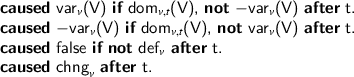
  If $\textsf {wr}(t)(v)$ contains a single element d, then the assignment is deterministic and the first three rules above can be substituted with⁴

  

Guards. To each subformula $\varphi$ of transition guards is associated a fluent $\text {grd}_{\varphi }$ that is true when the corresponding formula is satisfied. To simplify the notation, for any transition t, we will use $\text {grd}_{t}$ to indicate the fluent $\text {grd}_{\textsf {gd}(t)}$. Executability of transitions is conditioned to the satisfiability of their guards; instead of modifying the executability rule including the $\text {grd}_{t}$ among the preconditions, we use a constraint rule preventing executions of the action whenever its guard is not satisfied:

Translation of atoms ($\xi$) is defined in terms of $\text {var}_{v}$ predicates. For instance $\xi (v = w)$ corresponds to $\mathsf {var}_{v}(\mathsf {V})$, $\mathsf {var}_{w}(\mathsf {W})$, $\mathsf {V == W}$. That is $\xi (v,T) = \text {var}_{t} (\mathsf {T})$ for $t\in \mathcal {V}$, and $\xi (d,T) = \text {var}_{t} \mathsf {T ==}$ d for $d\in \bigcup _i \varDelta _i$. For each subformula $\varphi$ of transition guards a static rule is included to “define” the fluent $\text {grd}_{\varphi }$:

5.3 Correctness and Completeness

We provide a sketch of the correctness and completeness of the encoding. Proofs can be found in [5].

Planning states include all the information to reconstruct the original DAW-net states. In fact, we can define a function $\varPhi (\cdot )$ mapping consistent planning states into DAW-net states as following: $\varPhi (s) = (M,\eta )$ with

$$\begin{aligned} \forall p\in P,\; M(p) = {\left\{ \begin{array}{ll} 1 \text { if } p \in s \\ 0 \text { otherwise} \end{array}\right. } \quad \eta = \{ (v,d)\mid \text {var}_{v} (d)\in s \} \end{aligned}$$

$\varPhi (s)$ is well defined because s it cannot be the case that $\{ \text {var}_{v} (d), \text {var}_{v} (d') \}\subseteq s$ with $d\ne d'$, otherwise the static rule

would not be satisfied. Moreover, 1-safeness implies that we can restrict to markings with range in $\{0,1\}$. By looking at the static rules we can observe that those defining the predicates $\text {def}_{v}$ and $\text {grd}_{t}$ are stratified. Therefore their truth assignment depends only on the extension of $\text {var}_{v} (\cdot )$ predicates. This implies that $\text {grd}_{t}$ fluents are satisfied iff the variables assignment satisfies the corresponding guard $\textsf {gd}(t)$. Based on these observations, the correctness of the encoding is relatively straightforward since we need to show that a legal transition in the planning domain can be mapped to a valid firing. This is proved by inspecting the dynamic rules.

Lemma 3

(Correctness). Let W be a DAW-net and $\varOmega {(}W)$ the corresponding planning problem. If $\langle {s,\{t\},s'}\rangle$ is a legal transition in $\varOmega {(}W)$, then $\varPhi (s) {\mathop {\rightarrow }\limits ^{{t}}} \varPhi (s')$ is a valid firing of W.

The proof of completeness is more complex because – given a valid firing – we need to build a new planning state and show that it is minimal w.r.t. the transition. Since the starting state s of $\langle {s,\{t\},s'}\rangle$ does not require minimality we just need to show its existence, while $s'$ must be carefully defined on the basis of the rules in the planning domain.

Lemma 4

(Completeness). Let W be a DAW-net, $\varOmega {(}W)$ the corresponding planning problem and $(M,\eta ){\mathop {\rightarrow }\limits ^{{t}}}(M',\eta ')$ be a valid firing of W. Then for each consistent state s s.t. $\varPhi (s) = M$ there is a consistent state $s'$ s.t. $\varPhi (s') =M'$ and $\langle {s,\{t\},s'}\rangle$ is a legal transition in $\varOmega {(}W)$.

Lemmata 3 and 4 provide the basis for the inductive proof of the following theorem:

Theorem 2

Let W be a safe WF-net and $\varOmega {(}PN)$ the corresponding planning problem. Let $(M_0,\eta _0)$ be the initial state of W – i.e. with a single token in the source and no assignments – and $s_0$ the planning state satisfying the initial condition.

$(\Rightarrow )$ :

For any case $\zeta : (M_0,\eta _0) {\mathop {\rightarrow }\limits ^{{t_1}}} (M_1,\eta _1) \ldots (M_{n-1},\eta _{n-1}){\mathop {\rightarrow }\limits ^{{t_n}}} (M_{n},\eta _{n})$ in W there is a trajectory $\eta : \langle {s_0,\{t_1\},s_1}\rangle , \ldots , \langle {s_{n-1},\{t_n\},s_{n}}\rangle$ in $\varOmega {(}W)$ such that $(M_i,\eta _i) = \varPhi (s_i)$ for each $i \in \{0 \ldots n\}$ and viceversa.

$(\Leftarrow )$ :

For each trajectory $\eta : \langle {s_0,\{t_1\},s_1}\rangle , \ldots , \langle {s_{n-1},\{t_n\},s_{n}}\rangle$ in $\varOmega {(}W)$, the sequence of firings $\zeta : \varPhi (s_0) {\mathop {\rightarrow }\limits ^{{t_1}}} \varPhi (s_1) \ldots \varPhi (s_{n-1}) {\mathop {\rightarrow }\limits ^{{t_n}}} \varPhi (s_{n})$ is a case of W.

Theorem 2 above enables the exploitation of planning techniques to solve the reachability problem in DAW-net. Indeed, to verify whether the final marking is reachable it is sufficient to encode it as a condition for the final state and verify the existence of a trajectory terminating in a state where the condition is satisfied. Decidability of the planning problem is guaranteed by the fact that domains are effectively finite, as in Definition 9 the $\textsf {wr}$ functions range over a finite subset of the domain and by the fact that the planner takes as input the maximum length of the plan to be returned (note that this allows for dealing with loops).

6 Related Work and Conclusions

The key role of data in the context of business processes has been recently recognized.

A number of variants of PNs have been enriched so as to make tokens able to carry data and transitions aware of the data, as in the case of Workflow nets enriched with data [10, 15], the model adopted by the business process community. In  [15] Workflow Net transitions are enriched with information about data (e.g., a variable request) and about how it is used by the activity (for reading or writing purposes). Nevertheless, these nets do not consider data values (e.g., in the example of Sect. 2.2 we would not be aware of the values of the variable request that T4 is enabled to write). They only allow for the identification of whether the value of the data element is defined or undefined, thus limiting the reasoning capabilities that can be provided on top of them. For instance, in the example of Sect. 2.2, we would not be able to discriminate between the worker and the student loan for the trace in Sect. (2.2), as we would only be aware that request is defined after T4.

The problem of incomplete traces has been investigated in a number of works of trace alignment in the field of process mining, where it still represents one of the challenges. Several works have addressed the problem of aligning event logs and procedural models, without [2] and with [10, 11] data. All these works, however, explore the search space of possible moves in order to find the best one aligning the log and the model. Differently from them, we assume that the model is correct and we focus on the repair of incomplete execution traces. Moreover, we exploit state-of-the-art planning techniques to reason on control and data flow rather than solving an optimisation problem.

We can overall divide the approaches facing the problem of reconstructing flows of model activities given a partial set of information in two groups: quantitative and qualitative. The former rely on the availability of a probabilistic model of execution and knowledge. For example, in [14], the authors exploit stochastic PNs and Bayesian Networks to recover missing information (activities and their durations). The latter stand on the idea of describing “possible outcomes” regardless of likelihood; hence, knowledge about the world will consist of equally likely “alternative worlds” given the available observations in time, as in this work. For example, in [3] the same issue of reconstructing missing information has been tackled by reformulating it in terms of a Satisfiability(SAT) problem rather than as a planning problem.

Planning techniques have already been used in the context of business processes, e.g., for the construction and adaptation of autonomous process models [13]. In [4] automated planning techniques have been applied for aligning execution traces and declarative models. As in this work, in [6], planning techniques have been used for addressing the problem of incomplete execution traces with respect to procedural models.

However, differently from the two approaches above, this work uses for the first time planning techniques to target the problem of completing incomplete execution traces with respect to a procedural model that also takes into account data and the value they can assume.

Despite this work mainly focuses on the problem of trace completion, the proposed automated planning approach can easily exploit reachability for model satisfiability and trace compliance and furthermore can be easily extended also for aligning data-aware procedural models and execution traces. Moreover, the presented encoding in the planning language $\mathcal {K}$, can be directly adapted to other action languages with an expressiveness comparable to $\mathcal {C}$ [12]. In the future, we would like to explore these extensions and implement the proposed approach and its variants in a prototype.

References

Aalst, W.M.P.: Verification of workflow nets. In: Azéma, P., Balbo, G. (eds.) ICATPN 1997. LNCS, vol. 1248, pp. 407–426. Springer, Heidelberg (1997). https://doi.org/10.1007/3-540-63139-9_48
Adriansyah, A., van Dongen, B.F., van der Aalst, W.: Conformance checking using cost-based fitness analysis. In: Proceedings of the 2011 IEEE 15th International Enterprise Distributed Object Computing Conference (EDOC 2011), pp. 55–64. IEEE Computer Society (2011)
Bertoli, P., Di Francescomarino, C., Dragoni, M., Ghidini, C.: Reasoning-based techniques for dealing with incomplete business process execution traces. In: Baldoni, M., Baroglio, C., Boella, G., Micalizio, R. (eds.) AI*IA 2013. LNCS (LNAI), vol. 8249, pp. 469–480. Springer, Cham (2013). https://doi.org/10.1007/978-3-319-03524-6_40
De Giacomo, G., Maggi, F.M., Marrella, A., Sardiña, S.: Computing trace alignment against declarative process models through planning. In: Proceedings of the 26th International Conference on Automated Planning and Scheduling, pp. 367–375. AAAI Press (2016)
De Masellis, R., Di Francescomarino, C., Ghidini, C., Tessaris, S.: Enhancing workflow-nets with data for trace completion (2017). https://arxiv.org/abs/1706.00356
Di Francescomarino, C., Ghidini, C., Tessaris, S., Sandoval, I.V.: Completing workflow traces using action languages. In: Zdravkovic, J., Kirikova, M., Johannesson, P. (eds.) CAiSE 2015. LNCS, vol. 9097, pp. 314–330. Springer, Cham (2015). https://doi.org/10.1007/978-3-319-19069-3_20
Eiter, T., Faber, W., Leone, N., Pfeifer, G., Polleres, A.: A logic programming approach to knowledge-state planning, II: the DLVK system. Art. Intell. 144(1–2), 157–211 (2003)
van Hee, K., Sidorova, N., Voorhoeve, M.: Soundness and separability of workflow nets in the stepwise refinement approach. In: van der Aalst, W.M.P., Best, E. (eds.) ICATPN 2003. LNCS, vol. 2679, pp. 337–356. Springer, Heidelberg (2003). https://doi.org/10.1007/3-540-44919-1_22
Kiepuszewski, B., ter Hofstede, A.H.M., Bussler, C.J.: On structured workflow modelling. In: Bubenko, J., Krogstie, J., Pastor, O., Pernici, B., Rolland, C., Sølvberg, A. (eds.) Seminal Contributions to Information Systems Engineering. Springer, Heidelberg (2013)
de Leoni, M., van der Aalst, W.: Data-aware process mining: discovering decisions in processes using alignments. In: Proceedings of the 28th ACM Symposium on Applied Computing (SAC 2013), pp. 1454–1461. ACM (2013)
de Leoni, M., van der Aalst, W.M.P., van Dongen, B.F.: Data- and resource-aware conformance checking of business processes. In: Abramowicz, W., Kriksciuniene, D., Sakalauskas, V. (eds.) BIS 2012. LNBIP, vol. 117, pp. 48–59. Springer, Heidelberg (2012). https://doi.org/10.1007/978-3-642-30359-3_5
Lifschitz, V.: Action languages, answer sets and planning. In: Apt, K.R., Marek, V.W., Truszczynski, M., Warren, D.S. (eds.) The Logic Programming Paradigm: A 25-Year Perspective, pp. 357–373. Springer, Heidelberg (1999)
Marrella, A., Russo, A., Mecella, M.: Planlets: automatically recovering dynamic processes in YAWL. In: Meersman, R., Panetto, H., Dillon, T., Rinderle-Ma, S., Dadam, P., Zhou, X., Pearson, S., Ferscha, A., Bergamaschi, S., Cruz, I.F. (eds.) OTM 2012. LNCS, vol. 7565, pp. 268–286. Springer, Heidelberg (2012). https://doi.org/10.1007/978-3-642-33606-5_17
Rogge-Solti, A., Mans, R.S., van der Aalst, W.M.P., Weske, M.: Improving documentation by repairing event logs. In: Grabis, J., Kirikova, M., Zdravkovic, J., Stirna, J. (eds.) PoEM 2013. LNBIP, vol. 165, pp. 129–144. Springer, Heidelberg (2013). https://doi.org/10.1007/978-3-642-41641-5_10
Sidorova, N., Stahl, C., Trčka, N.: Soundness verification for conceptual workflow nets with data. Inf. Syst. 36(7), 1026–1043 (2011)
van der Aalst, W., van Hee, K., ter Hofstede, A., Sidorova, N., Verbeek, H., Voorhoeve, M., Wynn, M.: Soundness of workflow nets: classification, decidability, and analysis. Formal Aspects of Comput. 23(3), 333–363 (2010)
Acknowledgments
This research has been partially carried out within the Euregio IPN12 KAOS, which is funded by the “European Region Tyrol-South Tyrol-Trentino” (EGTC) under the first call for basic research projects.
Author information
Authors and Affiliations
Corresponding author
Editor information
Editors and Affiliations
Rights and permissions
Copyright information
© 2018 Springer International Publishing AG
About this paper
Cite this paper
De Masellis, R., Di Francescomarino, C., Ghidini, C., Tessaris, S. (2018). Enhancing Workflow-Nets with Data for Trace Completion. In: Teniente, E., Weidlich, M. (eds) Business Process Management Workshops. BPM 2017. Lecture Notes in Business Information Processing, vol 308. Springer, Cham. https://doi.org/10.1007/978-3-319-74030-0_6
Download citation
DOI: https://doi.org/10.1007/978-3-319-74030-0_6
Published:
Publisher Name: Springer, Cham
Print ISBN: 978-3-319-74029-4
Online ISBN: 978-3-319-74030-0
eBook Packages: Computer ScienceComputer Science (R0)