
Abstract
Treemaps has been used as diagrams in cartography to visualize hierarchical, multivariate, and time series data through the construction of hierarchies. Several algorithms exist for generating Treemaps. Despite the popularity of the Treemap, few studies have analyzed the effectiveness and efficiency of different algorithms. A user study was conducted to evaluate the slice-and-dice, squarified, ordered, strip, and ordered squarified algorithms. In the user study, the accuracy and response time for completing tasks were recorded. The slice-and-dice algorithm was identified as most suitable to represent true hierarchy (intrinsic hierarchy), followed by pivot-by-size. Slice-and-dice was also identified as the most suitable algorithm for representing false hierarchy (imposed hierarchy). When representing time series, slice-and-dice, strip, and ordered squarified algorithms were all determined to be suitable.
Access provided by CONRICYT-eBooks. Download conference paper PDF
Keywords
1 Introduction
Investigation on new representation methods has been one of the focuses of cartography. Treemap , a technique for visualizing hierarchical data has also been used in cartography to visualize socio-economic and demographic data. Treemap is suitable for detecting outliers, analyzing cause and effect, and discovering trends, and it has been successfully used to visualize various kinds of data, such as business information (Vliegen et al. 2006), electoral data (Wood et al. 2011), and social networks (Sathiyanarayanan and Burlutskiy 2015).
Because Treemap was originally designed to visualize hierarchical data, it can naturally be used to represent statistical data with spatial, temporal, or semantic hierarchies in cartography; for example, Jern et al. (2009) dynamically linked a Treemap to a choropleth map to facilitate the visualization of statistical data with a spatial hierarchy, while Slingsby et al. (2010a) used a Treemap to discover traffic patterns with a spatial hierarchy and visualize population data with a sematic hierarchy. Through construction of a false hierarchy (imposed hierarchy), Treemap can also be used to visualize multivariate statistical data and discovery correlation among different variables (Slingsby et al. 2010b), or to visualize flows and identify their spatial patterns (Wood et al. 2010).
Treemaps can be generated by several algorithms. These algorithms differ greatly in layout and may be suitable for different research questions or data types. Usability studies and controlled experiments are important in evaluating visualization techniques, because they help illustrate the potential benefits and limitations of visualization techniques as well as forming guidelines for their use (Plaisant 2004). Slingsby et al. (2009) proposed guidelines for a wide range of applications for designing Treemaps based on observations and experiences. Kong et al. (2010) proposed a set of design guidelines for creating effective rectangular Treemaps, concentrating on the design parameters of aspect ratio and luminance. The data represented in cartography is quite different from other kinds of data because it is spatially referenced and needs to be compared between different regions; therefore, the appropriate types of Treemap used as diagrams in cartography may vary in terms of the represented data and task types. Yet, little attention has been paid to it. Therefore, it is of interest to conduct a systematic evaluation on the effectiveness of different Treemap algorithms.
2 Treemap : A Brief Review
Treemaps can be generated by a variety of algorithms that can be classified into the three types listed in Table 1 based on their major design dimensions and salient characteristics.
-
Keep input data order only. Visual ordering in Treemaps is strictly consistent with one-dimensional ordering of the input data.
-
Keep low aspect ratio only. A low aspect ratio is preserved without considering the mapping between input data order and visual ordering.
-
Keep balance between input data order and low aspect ratio. The input data order (one-dimensional ordering or two-dimensional ordering) is preserved to some extent while maintaining a relatively low aspect ratio.
Our study concentrated on using Treemaps as diagrams to represent statistical data of individual regions. Geo-references can then be added through a point diagram map, a diagram map, a point grid map (Zhou et al. 2016) or a spatially ordered Treemap. This paper considers spatially ordered and Nmap algorithms to be methods for arranging nodes according to their geographic location rather than diagrams to represent statistical data of individual regions; therefore, these algorithms are not included in the user study . In the remaining types of Treemaps, we chose the algorithms that are used in existing Treemap software, such as treeMappa (http://www.treemappa.com/) and Treemap (https://www.treemap.com/). Therefore, slice-and-dice, squarified, ordered (including pivot-by-middle, pivot-by-split-size, and pivot-by size), strip, and ordered squarified algorithms are evaluated here (see Fig. 1), and they cover all three types listed in Table 1. The ordered algorithm could not be illustrated by a simple graph, so it is not shown in Fig. 1.

An illustration of different Treemap types. The number of each rectangle indicates the order of data input
3 Data Types Represented by Treemaps
Treemap algorithms differ greatly in the layouts, each suitable for different types of data. They are mainly used to represent true hierarchical, false hierarchical or spatio-temporal data , also called time series (Slingsby et al. 2009, 2010a, b).
-
True hierarchy (intrinsic hierarchy)
True hierarchy expresses the notion of a subtype of another type. An instinctive parent-child relationship exists between superior and subordinate elements. For instance, consumption can be classified into eight categories. These eight categories can be further classified into sub-categories, finally producing a two-level hierarchy.
-
False hierarchy (imposed hierarchy)
False hierarchy reconfigures a dataset with several independent attributes that lack an intrinsic parent-child relationship, producing multivariate data. For example, a Treemap can show the two independent attributes of consumption and income level, which have no intrinsic parent-child relationship and are therefore called a false hierarchy. This type of hierarchy can be used to represent potential relationships between two independent variables.
-
Time series
Temporal data represent a distinct example of a true hierarchy. Increasing or decreasing trends or periodic changes can be intuitively conveyed by a Treemap.
4 User Study Design
A user study was conducted to evaluate the effectiveness and efficiency of different Treemap algorithms applied to different types of data. First of all, users must receive the transmitted information completely and correctly (effectiveness). Secondly, the result must be assessed in relation to the amount of time required to achieve full and correct information (efficiency). The user study was conducted as a between-subjects test rather than a within-subjects test. This is because the answers corresponding to the last Treemap will influence the answers for the next Treemap as the same group is asked to read seven types of Treemaps and answer their corresponding questions. In the between-subjects test, subjects were equally divided into seven groups. Each group was asked to read a type of Treemap and answer the same series of questions. The answers and response times were recorded and analyzed to evaluate the various algorithms.
4.1 Visual Tasks for Treemap Cartography
Presentation and analysis are usually the primary communication goals of a representation. In order to achieve these goals, users must perform several visual tasks. The user study identified six visual tasks to be tested, based on the visualization operations (Wehrend 1993) and visual tasks (Zhou and Feiner 1998) as well as the characteristics of the three data types (see Table 2).
-
Element locating refers to finding special elements (rectangles) in Treemaps.
-
Visual comparison describes a comparison of an attribute that is mapped to visual variables on Treemaps of different objects. The visual comparison tasks mainly ask for the differences between the sizes of rectangles in this study.
-
Visual ranking requires the user to determine the order of elements (rectangles) according to special attributes. This task mainly asks for the differences between the sizes of rectangles in our study.
-
Characterize distribution provides a set of data cases and a quantitative attribute of interest, requiring the user to characterize the distribution of that attribute’s values over the set.
-
Correlation exploring refers to identifying potential relationships among multiple variants represented by Treemaps.
-
Trend detecting assesses the change patterns of objects over time, which can be described as increasing trends, decreasing trends, or periodic changes.
Element locating, visual comparison, visual ranking, and characterize distribution are the four basic visual tasks. The characterize distribution task may be initiated when the data contains a quantitative attribute. Correlation exploring is an important task for datasets characterized by false hierarchy. The final task, trend detecting, is used with time series.
4.2 Questionnaire Design
4.2.1 Dataset and Test Material
The questionnaire was divided into three parts (Part A, Part B, and Part C), corresponding to the three targeted types of data. When Treemaps are applied to cartography, different regions represented by Treemaps must be compared; therefore, the questionnaire used two represented regions to simulate comparisons. The Treemaps were made using treemappa (http://www.treemappa.com/), and the datasets used in the questionnaire and their corresponding Treemaps are as described below. The data came from 2011 Guangdong, Gansu, and Zhejiang Statistical Yearbook; and Data center of the Ministry of Environmental Protection of the People’s Republic of China (http://datacenter.mep.gov.cn/).
-
1.
Part A: True hierarchy (intrinsic hierarchy)
-
Dataset: Per capita annual consumption expenditure of urban households.
-
Treemap design: The proportions of the total expenditure of each province and consumption expenditure types are mapped by size and color, respectively (see Fig. 2).
Fig. 2 
Per capita annual consumption expenditure of urban households
-
-
2.
Part B: False hierarchy (imposed hierarchy)
-
Part B (a): One ordinal variable and one nominal variable
-

-
Dataset: Per capita annual consumption expenditure and construction of urban households by family income level.
-
Treemap design: Consumption expenditure by family income level (ordinal) forms the first-level, followed by consumption purpose (nominal) in the underlying level. Size represents the proportion of the total expenditure of each province and color indicates consumption purpose (see Fig. 3).
Fig. 3 
Per capita annual consumption expenditure of urban households by family income level

-
Part B (b): Two ordinal variables.
-
Dataset: Average education level of rural families with different income levels.
-
Treemap design: The proportion of total laborers by family income level (ordinal) constitutes the first-level, followed by education level (ordinal) in the underlying level. Size represents the proportion of total laborers of each province while color indicates the education levels (see Fig. 4).
Fig. 4 
Average education level of rural family’s laborers by family income level

-
3.
Part C: Time series
-
Dataset: Air quality levels.
-
Treemap design: The year is divided by months at the first level and days at the second level. The air quality level is mapped to color, while the sizes of the sub-rectangles are fixed. However, the squarified algorithm arranges rectangles according to their sizes. Therefore, we did not apply the squarified algorithm to this dataset (see Fig. 5).
Fig. 5 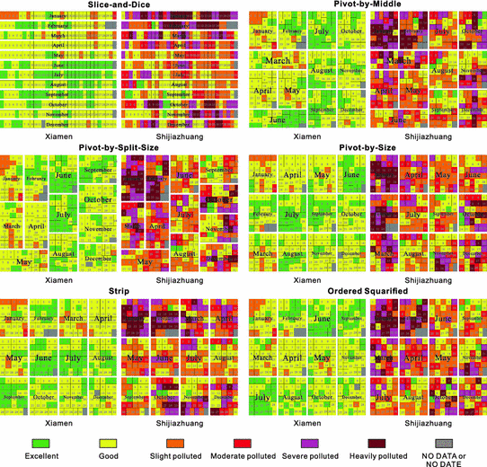
Air quality levels as depicted through Treemaps

4.2.2 Questions
We formulated several specific questions for each part based on the tasks listed in Table 2. When targeting rectangles in a visual comparison task, the difference between two rectangles cannot be obvious. To avoid subjects answering the questions based on existing knowledge without reading the Treemaps, some elements mentioned in questions and Treemaps were labeled using meaningless letters or numbers. Furthermore, several pilot trials were conducted before the user study . After the pilot trials, participants responded that the number of questions was too large and could cause visual fatigue and perfunctory psychology. Therefore, we deleted repeated tasks and their corresponding questions. Table 3 shows the final questionnaire. The complexity and difficulty of each part’s questions grow stepwise.
4.3 Procedure
The user study was conducted via a questionnaire on native HTML5 web pages. The subjects and questionnaires were equally divided into seven groups. Each subject was allowed to conduct the test independently before the deadline. The entire user study lasted for 14 days, from May 5, 2016 to May 19, 2016.
The first several pages of the web questionnaire contained detailed introductions to Treemaps and cartographic data, as well as instructions for answering. Each answer interface consisted of only one question with the corresponding Treemap placed under it. Subjects were asked to answer multiple-choice or free response without interruption. If subjects struggled to accomplish a task, they could choose the response “hard to tell or cannot tell.” After completing one question, subjects clicked a button to jump to the next question, repeating the process until the entire questionnaire was complete. Subjects could not return to previous pages to change their selections.
4.4 Subjects
The subjects were divided into seven groups. We invited subjects to participate in our study until the numbers of valid answer sheets from different groups were equal. Finally, the user study had 101 subjects in total, and we received 91 valid answer sheets from 54 females and 37 males. The subjects were found in school libraries randomly, each subject participated in the user study could get a gift, such as a notebook. Subjects had different academic backgrounds. They were asked to take a color vision test from Colblindor (http://www.color-blindness.com/color-arrangement-test/), and all reported normal color vision. In the brief background questionnaire, no participants reported using a Treemap before.
5 Results and Discussion
Response accuracy and response time—the indicators for evaluating the effectiveness and efficiency of Treemaps used as diagrams in cartography—were analyzed as follows.
We used one-way ANOVA test, Kruskal-Wallis test, and pairwise comparisons to analyze response time. Before analyzing response time, we conducted a Kolmogorov–Smirnov test between the response times of correct and incorrect answers for each question, concluding that there was no significant difference between the two groups in terms of response times. Therefore, we did not filter out the incorrect responses. As the response time distributions for most questions were skewed to the left, we first conducted lg-transformation to normalize the values (Ulrich and Miller 1993). If the P-value of the homogeneity test for variance was still less than 0.05 after lg-transformation, we used Kruskal-Wallis tests to analyze the group of response times; otherwise, we used the one-way ANOVA test. The entire analysis was executed in SPSS 20.0, with the results shown in Table 4. The significance tests reveal that the differences in response times between algorithms for most questions are statistically significant, except for Q2, Q6, Q7, and Q14.
Tables 5, 6, 7, 8, 9 and 10 show response accuracy and response time. The response times for Q2, Q6, Q7, and Q14 are not listed, because they lack statistical significance.
Element locating. The accuracy rate of the element locating tasks (Q1, Q8, and Q13) was 100% and is therefore not listed in Table 5. In Q1 and Q8, the results indicate that the slice-and-dice and strip algorithms took the least time. In Q1, the squarified algorithm took the longest time. And in Q13, pivot-by-split-size took the longest time. The capacity to retain the input data order and not change with data changes may influence the time required to accomplish elements locating tasks.
Visual comparison. As shown in Table 6, the slice-and-dice algorithm is most effective for completing visual comparison tasks, followed by the pivot-by-size and squarified algorithms based on the response accuracy. Overall, the evidence showing differences in response time is very weak. Results of response time in Q5 show that the slice-and-dice, strip, pivot-by-size, and ordered squarified algorithms take less time than pivot algorithms. Slice-and-dice takes the least time for Q9. However, the evidence is weak for the rest of the questions that address this task. The slice-and-dice Treemap fixes one side of each rectangle, making it much easier and more accurate to compare sizes. The pivot-by-size Treemap fixes one side of some rectangles, also making it easier to some extent. Although the squarified Treemap arranges sub-rectangles in order of size, which is helpful for recognizing the largest and smallest elements and making rough comparisons, accuracy is still lower than for the slice-and-dice Treemap.
Visual ranking. As shown in Table 7, results of Q6 indicate that the “F”, and order of the “HM,” “H,” and “M” rectangles are easy to recognize across all Treemaps. However, a small number of subjects did not see the “M” rectangle in the slice-and-dice and pivot-by-middle Treemaps, perhaps because this rectangle is too narrow to be observed. The results of the pivot-by-split-size algorithm show that more than half of mistakes occurred among the “R,” “TC,” and “RE” rectangles. Mistakes in Q7 occurred in comparisons among the “f1,” “f3,” “f5,” and “f6” rectangles, as well as in the comparison between the “f2” and “f9” rectangles and in the comparison between the “f7” and “f8” rectangles. Fixing one side of the sub-rectangles can help to complete the visual ranking task more easily and accurately. However, when very narrow sub-rectangles exist, the accuracy of the ranking task will decrease. Differences in response time for different algorithms were not significant. Overall, the slice-and-dice and pivot-by-size algorithms performed best in the ranking task.
Characterize distribution. As shown in Table 8, results indicate that slice-and-dice is the most effective algorithm based on the response accuracy, followed by strip and pivot-by-size. The slice-and-dice, strip, and ordered squarified algorithms are most efficient based on the response time. These results may mean that maintaining input order is crucial to the characterize distribution task.
Correlation exploring. As shown in Table 9, slice-and-dice is also the most effective algorithm for the correlation exploring task based on the response accuracy. In Q10, differences in response time among different algorithms were not significant, while in Q12, slice-and-dice took the least time. These results partially indicate that slice-and-dice is the most efficient algorithm. Slice-and-dice is suitable for detecting relationships between two independent variables. The reason could be that changes in attribute values do not cause changes in the structure of the slice-and-dice Treemap.
Trend detecting. As shown in Table 10, the slice-and-dice, strip, and ordered squarified algorithms performed better than the others in response accuracy. In Q15, the slice-and-dice and strip algorithms took less time. These results suggest that keeping relatively high consistency in input order and display order and displaying results in an order that users are accustomed to could be important to the trend detecting task.
6 Conclusion
This paper evaluated the effectiveness and efficiency of different Treemaps as diagrams in cartography. Considering both response time and response accuracy for each type of task, slice-and-dice is the most suitable algorithm to represent true hierarchy, followed by pivot-by-size; however, when very small rectangles occur in slice-and-dice, pivot-by-size works better. In representing false hierarchy, slice-and-dice is again the most suitable algorithm. When representing time series, the slice-and-dice, strip and ordered squarified algorithms are suitable. The evaluation results can be used as a guide for choosing Treemap algorithms.
The data that we evaluated contain only dozens of nodes, and the data are represented by static Treemaps. When the data volume increases, the data can be better represented by dynamic and interactive Treemaps. This study did not consider tasks for dynamic and interactive Treemaps. It is possible that both the effectiveness and efficiency of Treemap representation may change with the aid of good interaction, and this is the future work of our study.
References
Bederson, B. B., Shneiderman, B., & Wattenberg, M. (2003). Ordered and quantum treemaps: making effective use of 2d space to display hierarchies. ACM Transactions on Graphics, 21(4), 257–278.
Bruls, M., Huizing, K., & Van Wijk, J. J. (2000). Squarified treemaps. Data visualization 2000 (pp. 33–42). Vienna: Springer.
Duarte, F. S., Sikansi, F., Fatore, F. M., Fadel, S. G., & Paulovich, F. V. (2014). Nmap: A novel neighborhood preservation space-filling algorithm. IEEE Transactions on Visualization and Computer Graphics, 20(12), 2063–2071.
Jern, M., Rogstadius, J., Åström, T. (2009). Treemaps and choropleth maps applied to regional hierarchical statistical data. In 2009 13th International Conference Information Visualisation (pp. 403–410). IEEE.
Johnson, B., & Shneiderman, B. (1991). Tree-maps: A space-filling approach to the visualization of hierarchical information structures. In IEEE Conference on Visualization, 1991. Visualization’91, Proceedings (pp. 284–291). IEEE.
Kong, N., Heer, J., & Agrawala, M. (2010). Perceptual guidelines for creating rectangular treemaps. IEEE Transactions on Visualization and Computer Graphics, 16(6), 990–998.
Plaisant, C. (2004). The challenge of information visualization evaluation. In Proceedings of the Working Conference on Advanced Visual Interfaces (pp. 109–116). ACM.
Sathiyanarayanan, M., & Burlutskiy, N. (2015). Visualizing social networks using a treemap overlaid with a graph. Procedia Computer Science, 58, 113–120.
Shneiderman, B., & Wattenberg, M. (2001). Ordered treemap layouts. In Proceedings of the IEEE Symposium on Information Visualization 2001 (Vol. 73078).
Slingsby, A., Dykes, J., & Wood, J. (2009). Configuring hierarchical layouts to address research questions. IEEE Transactions on Visualization and Computer Graphics, 15(6), 977–984.
Slingsby, A., Wood, J., & Dykes, J. (2010a). Treemap cartography for showing spatial and temporal traffic patterns. Journal of Maps, 6(1), 135–146.
Slingsby, A., Dykes, J., & Wood, J. (2010b). Rectangular hierarchical cartograms for socio-economic data. Journal of Maps, 6(1), 330–345.
Tu, Y., & Shen, H. W. (2007). Visualizing changes of hierarchical data using treemaps. IEEE Transactions on Visualization and Computer Graphics, 13(6), 1286–1293.
Ulrich, R., & Miller, J. (1993). Information processing models generating lognormally distributed reaction times. Journal of Mathematical Psychology, 37(4), 513–525.
Vliegen, R., Van Wijk, J. J., & Van der Linden, E. J. (2006). Visualizing business data with generalized treemaps. IEEE Transactions on Visualization and Computer Graphics, 12(5), 789–796.
Wattenberg, M. (1999). Visualizing the stock market. In CHI’99 extended abstracts on human factors in computing systems (pp. 188–189). ACM.
Wood, J., Badawood, D., Dykes, J., & Slingsby, A. (2011). BallotMaps: Detecting name bias in alphabetically ordered ballot papers. IEEE Transactions on Visualization and Computer Graphics, 17(12), 2384–2391.
Wood, J., & Dykes, J. (2008). Spatially ordered treemaps. IEEE Transactions on Visualization and Computer Graphics, 14(6), 1348–1355.
Wood, J., Dykes, J., & Slingsby, A. (2010). Visualisation of origins, destinations and flows with OD maps. The Cartographic Journal, 47(2), 117–129.
Wehrend, S. (1993). Appendix B: Taxonomy of visualization goals (pp. 187–199). Visual cues: Practical data visualization.
Zhou, M. X., & Feiner, S. K. (1998). Visual task characterization for automated visual discourse synthesis. In Proceedings of the SIGCHI Conference on Human Factors in Computing Systems (pp. 392–399). ACM Press/Addison-Wesley Publishing Co.
Zhou, M., Tian, J., Xiong, F., & Wang, R. (2016). Point grid map: A new type of thematic map for statistical data associated with geographic points. Cartography and Geographic Information Science, 1–16.
Acknowledgements
We appreciate the suggestions and comments from Michael Peterson and the anonymous reviewers. Our work was supported by the Special Program for Basic Science of China under Grant No. 2013FY112800.
Author information
Authors and Affiliations
Corresponding author
Editor information
Editors and Affiliations
Rights and permissions
Copyright information
© 2017 Springer International Publishing AG
About this paper
Cite this paper
Zhou, M., Cheng, Y., Ye, N., Tian, J. (2017). Effectiveness and Efficiency of Using Different Types of Rectangular Treemap as Diagrams in Cartography. In: Peterson, M. (eds) Advances in Cartography and GIScience. ICACI 2017. Lecture Notes in Geoinformation and Cartography(). Springer, Cham. https://doi.org/10.1007/978-3-319-57336-6_14
Download citation
DOI: https://doi.org/10.1007/978-3-319-57336-6_14
Published:
Publisher Name: Springer, Cham
Print ISBN: 978-3-319-57335-9
Online ISBN: 978-3-319-57336-6
eBook Packages: Earth and Environmental ScienceEarth and Environmental Science (R0)