Localization and Tracking in WSNs

Abstract

Localization—the process by which the positions of the nodes of a Wireless Sensor Network (WSN) are found with respect to some absolute or relative frame of reference—is fundamental to how the WSN performs at executing its functions.

These keywords were added by machine and not by the authors. This process is experimental and the keywords may be updated as the learning algorithm improves.

6.1 Introduction

Localization—the process by which the positions of the nodes of a Wireless Sensor Network (WSN) are found with respect to some absolute or relative frame of reference—is fundamental to how the WSN performs at executing its functions. Critical WSN operations such as routing (e.g., geographical routing), data aggregation and navigation (for mobile sensor networks) all heavily rely on the localization mechanism. For many of today’s systems or applications requiring localization functionality, the NAVSTAR Global Positioning System (GPS) is typically sufficient [1]. In WSNs, however, GPS-based methods fall short for two main reasons. First, effective operation of a GPS-based localization mechanism demands that the WSN system has line-of-sight communication with multiple satellites. This requirement is typically not realizable because most WSN applications are meant for environments inherently having obstructions to electromagnetic signals, e.g., in urban areas (i.e., in the midst of tall buildings), indoors, under water, in forests or in mountainous areas to mention but a few. The second challenge posed by GPS-based techniques is their prohibitive price—the cost of the full network can increase over tenfold if a small subset of the nodes is equipped with GPS receivers [17]. With GPS being unsuitable for the vast majority of WSN applications, research on localization in WSNs is mostly focused on GPS-less techniques, which overcome the challenges seen with a GPS.

In this chapter, we examine some of these techniques. We first explore the localization scenario where all nodes are stationary (i.e., the layout problem [9]). We later extend our discussion to the case where node mobility is involved (i.e., where some WSN nodes are mobile) and present the algorithms and extra design considerations, which are prompted by node mobility. We wind up the chapter with a brief discussion on object tracking in WSNs, a very closely related problem to localization.

6.2 Design and Evaluation of Localization Algorithms

To design or analyze the applicability of a localization algorithm to a given WSN application, one has to consider a range of factors, that include, the resource requirements of the algorithm, the topology of the network, the nature of the terrain in which the WSN will be deployed and the density of nodes in the network [2]. We discuss these factors in this sub-section.

Node Density

The density of nodes in the WSN has a major bearing on what kinds of localization algorithms are suited for the network. For hop-count based algorithms for instance, a high density of nodes is required to ensure accuracy of the approximated distances [2]. Where beacon nodes are part of the localization process, their density must be high enough for the localization operations to be effective. In general, many localization algorithms demand a certain threshold node density below which the localization error may increase significantly but above which the error reduces only very slightly. As an example, in a beacon-driven localization simulation based on 500 WSN nodes deployed in a 100 m × 100 m × 100 m area [28], it was found, for an anchor (or beacon) percentage of 20 %, that the localization coverage increased by almost 50 % when the node density (which was represented as the expected number of nodes in a node’s neighborhood) increased from 8 to 11, yet increased almost negligibly when the node density increased from 12 to 16.

Environmental Factors

Obstacles such as buildings, rocks, and trees in the area where the WSN is deployed can impede signals used for the measurement of signal ranges (ranging methods discussed in Sect. 6.3.1.1) and result in an erratic localization process. For example, signals reflected by physical obstacles located within the WSN may interfere with each other, resulting into multipath effects and associated localization errors [1]. Besides physical obstacles, other environmental factors such as precipitation and the amount of moisture in the air are well known to affect radio wave propagation, potentially causing errors for localization techniques that rely on radio waves [1]. A good localization algorithm should have mechanisms to guard against or recover from the errors caused by environmental factors such as those listed here.

Network Topology

Irregular WSN topologies typically result into higher localization errors [10]. Even where the topology may not be irregular, nodes at the edge of the WSN generally tend to be relatively difficult to localize since they: (1) have a small number of neighbors, and, (2) have all their neighbors on one side, which implies that range measurements for these nodes provide only a limited perspective of their location [2]. A good localization algorithm should be able to make the necessary compensations for errors resulting from topology artifacts.

Resource Constraints

The design of localization algorithms for WSNs must be cognizant of the fact that WSN nodes have limited processing power and memory. For applications where low precision of localization measurements is adequate, approximate algorithms that can estimate position using low power and cheap hardware offer a good option around the resource limitations challenge [15]. When an application requires localization information at a high precision, the exact algorithms needed for this purpose generally consume more power. A good algorithm in such a case would have to distribute localization tasks between different nodes (e.g., tasks split between the base station, beacon nodes (which are typically more powerful than the typical node) and the rest of the nodes).

6.3 Categorization of Localization Approaches

In terms of the algorithmic methodology used to make localization computations, localization algorithms in WSNs are categorized as either range-based or range-free. Range-based methods use estimates of distance or angles to localize the WSN’s nodes. From these measurements, simple geometric relationships are used to compute node locations without making assumptions about the underlying topology of the WSN. Range-free methods on the other hand rely on connectivity information in the WSN to estimate node locations. For effective localization, many range-free methods rely on the WSN’s topology meeting certain requirements (e.g., that hop distances have low variance). The main advantage of range-free methods is that they do not require specialized hardware for distance and angle measurements, which makes them cost-effective in comparison to range-based methods. The key advantage of range-based methods on the other hand is the fact that they tend to be more accurate in comparison to the range-free methods [9]. Regarding the way in which localization computations are undertaken, certain (range-free or range-based) localization algorithms perform their localization computations in a distributed manner, while others operate in a centralized fashion. The latter approach has the core localization computations running on dedicated nodes (e.g., base station), while the former has the core localization operations running on the individual nodes.

In this section we explore some of the most popular localization schemes in the literature. We discuss several prominent range-based and range-free algorithms in details, and then finally give a general comparison between the centralized and distributed design approaches for WSN localization algorithms.

6.3.1 Range-Based Methods

These methods operate in two steps: a measurement step in which the distance/angle measurements are made, and a computation step in which the recorded measurements are combined to do the actual localization. The four main approaches used in the measurement step¹ include Received Signal Strength Indicator (RSSI), Time of Arrival (ToA), Time Difference of Arrival (TDoA) and Angle of Arrival (AoA) and are discussed next before we present the computation approaches used in the final localization step.

6.3.1.1 Approaches to Making Ranging Measurements

Received Signal Strength Indicator (RSSI)

Theoretically, the power of a radio signal at a given point is known to be inversely proportional to the square of the distance of the point signal source. This relationship forms the backbone of the RSSI technique. If the power of the signal at the transmitting node is known, then, using this relationship, the receiving node can estimate its distance from the sending node. The main advantage of this approach is that it requires no dedicated hardware, i.e., it only requires the sensors to have a radio, which most WSN nodes are expected to have anyway. In practice, however, this approach is for several reasons susceptible to noise. Physical obstacles (e.g., walls, people, etc.) absorb and reflect the waves, while different environments impact the propagation of radio waves differently (e.g., radio waves propagate differently over asphalt than over grass [9]). With the many possible sources of error, radio wave measurements made in real settings rarely agree with the theoretical relationship between signal strength and distance traversed by the signal.

For example in [12], an experiment based on Intel’s crossbow motes revealed that RSSI measurements taken from different directions of the sensors (e.g., north, east, west) did not depict a consistent relationship with the distance from the sensors. In this particular experiment, researchers minimized potential sources of noise, e.g., sensors had their batteries fully powered up throughout the experiment, the surface on which the experiments were done was level, no physical obstacles were present and electronic equipment that could potentially cause interference were not present in the vicinity of the experimental apparatus. With this closely controlled environment failing to demonstrate the power of the RSSI-based ranging method, the research raised doubts about how well RSSI would perform in a real deployment in the wild. Several other studies have made similar findings on the ineffectiveness of RSSI as a ranging method for WSNs. As of today, research on the development of reliable RSSI-based methods for WSN localization continues to be ongoing.

Time of Arrival (ToA)

This method has two variants: One-Way Time-of-Arrival (OW-ToA) and Two-Way Time-of-Arrival (TW-ToA). In the OW-ToA approach, the sender and receiver of a signal have synchronized clocks. When the signal arrives at the receiver, it registers the time of arrival, and the time of transmission of the signal (this time is sent to the receiving node) and uses these two variables to compute the distance between the two nodes. The difference, $t_{ij}$, between the time of transmission of the signal at the sending node and the time of receipt at the receiving node can be obtained as (see [13]):

$$t_{ij} = \frac{{\left\| {x_{i} - x_{j} } \right\|}}{c} + e_{ij} ,$$

(6.1)

where $\left\| {x_{i} - x_{j} } \right\|$ is the actual distance between the two nodes, c is the signal propagation speed (which should be known for the medium in question) and $e_{ij}$ is the error term which follows the Gaussian distribution with zero mean and variance $\sigma_{ij}$. The distance estimate $d_{ij}$ is obtained from,

$$d_{ij} = ct_{ij} = \left\| {x_{i} - x_{j} } \right\| + ce_{ij} .$$

(6.2)

In general, a high Signal-to-Noise Ratio helps minimize the estimation error. Three major challenges faced by this method are: (1) it suffers from unreliable measurements in the event that the clocks go out of sync, (2) extra communication overhead is incurred as each source has to send the time of signal transmission to the receiver, (3) since radio signals travel at the speed of light, recording their time of arrival precisely is a challenge [1].

The TW-ToA approach eliminates the need to synchronize clocks as the distance between the communicating nodes is estimated based on the round-trip delay of the signal. The sensor node i sends a signal to the receiver node j. After a turn-around time $t_{j}^{a}$ the receiving node sends back a message to j to acknowledge receipt of the signal. Using a similar notation to that of the ToA method, the distance estimate $d_{ij}$ can be expressed as:

$$d_{ij} = \left\| {x_{i} - x_{j} } \right\| + ct_{i}^{a} + c\left( {\frac{{e_{ij} }}{2} + \frac{{e_{ji} }}{2}} \right),$$

(6.3)

where $e_{ij}$ and $e_{ji}$ are the estimation errors at nodes j and nodes i for the signals being transmitted from them. This method eliminates the error due to imprecise synchronization of the clocks on nodes i and j; however, the method is also susceptible to errors if the clock in the reference node undergoes a drift.

Time Difference of Arrival (TDoA)

This method computes the distance between two nodes based on the difference between the times of arrival of the radio signal and a second signal (typically an ultrasound or an audible frequency, which require each node to have a speaker and microphone [2]). The transmitter first sends a radio message, and then waits for an interval t before sending the sound wave. On receiving the radio signal, the receiving node switches on its microphone to detect the incoming audio signal. If the radio signal and audio signal are, respectively, received at times $t_{r}$ and $t_{s}$, the distance d between the two nodes can be estimated from

$$d = (c - v)(t_{s} - t_{r} - t),$$

(6.4)

where c and $v$ are, respectively, the propagation speed of sound and radio waves.

The TDoA concept can also be used with multiple sensors/receivers that are tasked with localizing a sensor node or a target in their sensing field. Consider a group of sensors shown in Fig. 6.1 and a hidden emitter that the WSN is trying to localize, i.e., consider a network of N sensors with coordinate vectors $\vec{p}_{i} (t)$, $i \in \left\{ {1,2, \ldots ,N} \right\}$, and a hidden emitter located at $\vec{p}_{e} (t)$. Included are only sensors that are selected to localize the specific emitter source/sensor node. The distance between the emitter and the sensor i is $r_{ei} (t)$.

Fig. 6.1

Sensor network localize the hidden emitter using TDoA framework

The TDoA sensing concept allows for measurement of difference in time of arrival, i.e.,

$$r_{ij} (t) = r_{ei} (t) - r_{ej} (t) = c(t_{i} - t_{j} ),$$

(6.5)

where c is the speed of a signal propagation, $r_{ei} (t)$ is the distance between the emitter and the i-th sensor, and $t_{i}$ is the signal propagation time between the emitter and the i-th sensor. Without a loss of generality, consider the coordinate system origin to be located at sensor 1. The closed form of TDoA-based localization is given in [18] using basic geometry of the sensor network

$$\left( {P_{e} + r_{ij} } \right)^{2} \,=\, \left\| {\vec{p}_{i} } \right\|^{2} \,-\, 2\vec{p}_{i} \vec{p}_{e} + P_{e}^{2} ,$$

(6.6)

where $P_{e}$ is the distance of the emitter from the coordinate system origin. This equation is equivalent to

$$0 = \left\| {\vec{p}_{i} } \right\|^{2} - 2\vec{p}_{i} \vec{p}_{e} - r_{ij}^{2} - 2P_{e} r_{ij} .$$

(6.7)

However, the TDoA measurements will produce errors in the above equation, yielding

$$\varepsilon_{i} = \left\| {\vec{p}_{i} } \right\|^{2} - 2\vec{p}_{i} \vec{p}_{e} - r_{ij}^{2} - 2P_{e} r_{ij} ,$$

(6.8)

or in the matrix form [18]

$$\vec{\varepsilon } = {\mathbf{P}} - 2{\mathbf{S}}\vec{p}_{e} - 2P_{e} {\mathbf{R}},$$

(6.9)

where matrices are defined as:

$${\mathbf{P}} = \left[ {\begin{array}{*{20}c} {\left\| {\vec{p}_{2} } \right\|^{2} \,-\, r_{21}^{2} } \\ {\left\| {\vec{p}_{3} } \right\|^{2} \,-\, r_{31}^{2} } \\ \vdots \\ {\left\| {\vec{p}_{N} } \right\|^{2} \,-\, r_{N1}^{2} } \\ \end{array} } \right],\quad {\mathbf{S}} = \left[ {\begin{array}{*{20}c} {x_{2} \,y_{2} \,z_{2} } \\ {x_{3} \,y_{3} \,z_{3} } \\ \vdots \\ {x_{N} \,y_{N} \,z_{N} } \\ \end{array} } \right],\quad {\mathbf{R}} = \left[ {\begin{array}{*{20}c} {r_{21} } \\ {r_{31} } \\ \vdots \\ {r_{N1} } \\ \end{array} } \right]$$

(6.10)

Note that the TDoA measurements will affect matrices ${\mathbf{P}}$ and ${\mathbf{R}}$, while matrix ${\mathbf{S}}$ contains locations of sensors. Then, the least-squares error solution for the optimal emitter location estimation is given by

$$\vec{p}_{e} = \frac{1}{2}\left( {{\mathbf{S}}^{T} {\mathbf{S}}} \right)^{ - 1} {\mathbf{S}}^{T} \left( {{\mathbf{P}} - 2P_{e} {\mathbf{R}}} \right).$$

(6.11)

This solution assumes that the distance of the emitter from the coordinate system origin $P_{e}$ is known. To get an optimal solution in terms of $\vec{p}_{e}$ only, one needs to optimize the modified Eq. (6.9) in terms of $P_{e}$. The modified Eq. (6.9) in given by

$$\vec{\varepsilon } = {\mathbf{P}} - {\mathbf{S}}\left( {{\mathbf{S}}^{T} {\mathbf{S}}} \right)^{ - 1} {\mathbf{S}}^{T} \left( {{\mathbf{P}} - 2P_{e} {\mathbf{R}}} \right) - 2P_{e} {\mathbf{R}},$$

(6.12)

$$\vec{\varepsilon } = \left( {{\mathbf{P}} - 2P_{e} {\mathbf{R}}} \right)\left( {{\mathbf{I}} - {\mathbf{S}}\left( {{\mathbf{S}}^{T} {\mathbf{S}}} \right)^{ - 1} {\mathbf{S}}^{T} } \right).$$

(6.13)

The closed-form solution is obtained by minimizing $\vec{\varepsilon}^{T} \vec{\varepsilon}$ and is given by

$$\vec{p}_{e} = \frac{1}{2}\left( {{\mathbf{S}}^{T} {\mathbf{S}}} \right)^{ - 1} {\mathbf{S}}^{T} \left( {{\mathbf{I}} - \frac{{{\mathbf{RR}}^{T} {\mathbf{S}}_{1} {\mathbf{S}}_{1} }}{{{\mathbf{R}}^{T} {\mathbf{S}}_{1} {\mathbf{S}}_{1} {\mathbf{R}}}}} \right){\mathbf{P}},$$

(6.14)

where ${\mathbf{S}}_{1} = {\mathbf{I}} - {\mathbf{S}}\left( {{\mathbf{S}}^{T} {\mathbf{S}}} \right)^{ - 1} {\mathbf{S}}^{T}$. It is recommended to first quickly calculate the emitter estimate and then to proceed with iterative methods for improved accuracy. Note that this method requires five or more sensors to accurately estimate the emitter location [18].

To minimize errors, TDoA requires that the media be free of echoes and the speakers be calibrated with the microphones since they tend to have different transmission and reception characteristics [2]. TDoA is considerably much more accurate than methods which entirely rely on radio waves. For the specific comparison between TDoA and RSSI, TDoA attains much better performance than RSSI because it only measures signal travel time yet RSSI measures signal magnitude. Signal magnitude measurements see noise from both occlusion and signal multipath effects, while signal time measurements only see noise from occlusion [2]. The major disadvantage of TDoA is the extra hardware it requires (e.g., microphones and speakers).

Angle of Arrival (AoA)

This method uses several spatially separated radio or microphone arrays on the WSN node. When a WSN node receives a signal, differences between the phase of the signal at different microphones are used to determine the location of the transmitter. Increasing the number of array elements, the distance between them and the SNR helps improve the performance of the AoA method [13]. In a 2-dimensional setting without noise, a minimum of two receivers can be used to locate the transmitter. The presence of noise calls for the usage of more than two AoA measurements. The major challenge with the AoA technique is the expensive and bulky hardware (microphone and several speakers) it requires [2]. Moreover, the small form factor of the WSN nodes makes it difficult to accommodate multiple speakers that have enough separation as required for good performance.

6.3.1.2 Computing Locations from Ranging Measurements

From the angle and distance measurements, the most commonly used methods to find the locations of the WSN nodes are angulation, lateration, and statistical estimation. Angulation uses measured angles between nodes while lateration uses distance measurements between nodes to localize the nodes. For statistical estimation, the most commonly used techniques are Maximum Likelihood Estimation (MLE) and Bayesian inference. We next briefly discuss the mechanisms of these techniques.

Angulation

This method is used when the angles or bearings of the nodes to be localized are known relative to the known locations of the anchor (or beacon) nodes (e.g., after application of the AoA technique). Triangulation is a specific form of angulation in which the angular separation between two anchors and the target node are used to localize the target node.

Figure 6.2 illustrates the triangulation mechanism. The two anchor nodes (Anchor #1 and Anchor #2) are at known positions and hence at a known distance, L, apart. Angles α and β represent the angular displacement of the target node from the two anchors. As illustrated in the Fig. 6.2, the meeting point of the two lines from the anchor determines the location of the target node. This location could for instance be expressed in terms of d, the perpendicular distance of the target node from the line joining the two anchors. Using simple trigonometry, d can be obtained using the following equation

$$d\left( {\frac{1}{{{ \tan }\,\alpha }} + \frac{1}{{{ \tan }\,\beta }}} \right) = L,$$

(6.15)

which can be rewritten as

$$d = \frac{{L\,{ \sin }\,\alpha \,{ \sin }\,\beta }}{{{ \sin }(\alpha + \beta )}}.$$

(6.16)

Fig. 6.2

Illustration of triangulation

In practice, the angular measurements α and β can be noisy, and the procedure can only define regions in which the target node is likely to be located. Angulation computations involving other nodes may then be used to fine-tune the position estimate.

Lateration

This method is used when ranges between the target node and the anchor positions are known. Figure 6.3 illustrates trilateration, a form of lateration in which three anchor nodes are used to locate the target node. For instance, if ranging measurements reveal that the target node is a distance R ₁ from the anchor node #1, the method stipulates that a circle of radius R ₁ be drawn around #1, with the circumference of the circle defining the set of points where the target node could be located.

Fig. 6.3

Illustration of trilateration

With a similar process undertaken for the other three anchors, the point of intersection of the three circles represents the location of the target node. Assuming the center of the circle with radius R ₁ (i.e., the center of the circle around anchor #1) has the coordinates (x ₁, y ₁) with the centers and radii of the circles around anchors #2 and #3 defined similarly, the position (x, y) of the target node is found from the solution of the following three equations of the respective circles:

$$(x - x_{i} )^{2} + (y - y_{i} )^{2} = R_{i}^{2} ,\quad i = 1,2,3.$$

(6.17)

Similarly as for angulation, measurement errors make it difficult to obtain the precise position of the target node. In such cases a region in which the target node is located is what is returned by the trilateration algorithm (as opposed to a precise point).

Estimation

These methods use a measurement model expressing the relationship between the state of the system and measured data [1]. In Maximum Likelihood Estimation (MLE), the parameters capturing the system state are obtained by maximizing the likelihood of the measured data. The parameters are estimated using measured data with no prior information about state used. In Bayesian inference on the other hand, the system is estimated using both prior information and measured data. The estimation is based on recursive iteration, which use Bayes theorem [1].

6.3.2 Range-Free Methods

At the cost of reduced localization accuracy relative to the range-based techniques, range-free methods are designed to operate without the need for expensive hardware (e.g., the speakers and microphones used in TDoA). The idea behind this design approach is that the required localization precision for certain applications may not be so high to warrant the huge cost associated with the usage of expensive hardware on the nodes [6]. Range-free localization techniques can be generalized into three categories, namely, anchor proximity based methods, connectivity-based methods and event-driven methods [27]. In this section, we briefly discuss each of these categories and give examples of some of the most prominent algorithms in each category.

6.3.2.1 Anchor Proximity Based Methods

Localization under this approach is based on coarse-grained information of whether a given node is within the vicinity of another node. Based on a modality such as radio, infrared or sound, this localization approach uses binary information on whether a node A is within range of another node B, and then uses this information (in conjunction with similar information from other nodes) to carry out localization for the whole network.

The simplest example of an anchor proximity based localization method is the Centroid method [3, 27]. The method assumes a network in which a set of anchor nodes located at known positions (x ₁, y ₁) through (x _n , y _n ) form a regular mesh and transmit signals containing their positions to the rest of the nodes. Each anchor node i is associated with a connectivity metric CM _i which is computed using

$${\text{CM}}_{i} = \frac{{N_{\text{rec}} (i,t)}}{{N_{\text{snt}} (i,t)}} \times 100,$$

(6.18)

where $N_{\text{rec}} (i,t)$ is the number of beacons sent by i which have been received in time t, and $N_{\text{snt}} (i,t)$ is the number of beacons that have been sent by i in time t. Based on signals received from a subset of k anchors having ${\text{CM}}_{i}$ exceeding a certain threshold ${\text{CM}}_{\text{th}}$, a node estimates its location, $(\hat{x},\hat{y})$ as the centroid of the reference points, i.e.

$$(\hat{x},\hat{y}) = \left( {\frac{\sum_{\{j|CM_j \geq CM_{th}\}} x_{j}}{k},\frac{{\sum_{\{j|CM_j \geq CM_{th}\}} y_{j}}}{k}} \right).$$

(6.19)

To minimize the localization error, the method requires a dense network of anchors. Variants of this baseline Centroid localization algorithm incorporate additional heuristics, such as the use of weights to give more prominence to anchors closer to the node in question (see survey in [27]).

Another widely studied anchor-based algorithm is the Approximate Point in Triangle (APIT) algorithm [6]. This method segments the WSN into triangular regions whose vertices are the locations of anchor nodes. A node is localized based on the triangles to which it is found to belong. The method can be subdivided into three steps: (1) Beacon exchange—in this step nodes receive beacons from anchor nodes, (2) Point In Triangle (PIT) Testing—here a node chooses three anchors from all anchors from which it has received beacons and tests whether it is inside the triangle formed by connecting these anchors (this process repeats until all combinations are exhausted or the required accuracy is achieved), (3) APIT aggregation and centroid calculation—which involves the combination of results from different PIT tests to determine which triangle segments are more likely to contain a node, followed by a centroid computation which determines the location of the node.

Figure 6.4 illustrates how the results from multiple PIT tests are aggregated. A grid array is used to represent the area of the region that a node could occupy. The smaller the size of the grids, the better the accuracy. When a PIT test determines that a node lies inside a given triangle, all cells in that triangle have their score incremented. When the node is found to lie outside a given triangle, the scores of the cells inside that triangle are decremented. At the end of the process, the overlapping area with maximum score is used to calculate the centroid similar to (6.19). This method also requires a high density of anchors for good performance. Several variants of this method exist in the literature with a focus on attributes such as anchor self-placement and optimization for WSNs with different properties [27].

Fig. 6.4

Scan algorithm for PIT aggregation

6.3.2.2 Connectivity-Based Methods

Connectivity-based methods utilize connectivity information across the network to make localization decisions. One of the most prominent amongst these methods is the DV-hop method [11]. This method is centered on the distance vector routing paradigm. Each anchor broadcasts a beacon that contains its location. The beacon has its hop-count parameter initialized to one and incremented at each hop. As the beacons from multiple anchors traverse the network, each node on their path registers the minimum hop-count value per anchor. Anchor nodes also keep track of this information from beacons originating from their fellow anchors. If ${\text{dis}}(v_{i} ,v_{j} )$ and ${\text{hop}}(v_{i} ,v_{j} )$ denote the physical distance and a minimum number of hops between anchors v _i and v _j  respectively, the anchors estimate the average size of a hop, D _hop, using

$$D_{\text{hop}} = \frac{{\sum\nolimits_{i \ne j} {{\text{dis}}(v_{i} ,v_{j} )} }}{{\sum\nolimits_{i \ne j} {{\text{hop}}(v_{i} ,v_{j} )} }}.$$

(6.20)

Using this information, an arbitrary node u _k can estimate its physical distance to the anchor v _i using

$${\text{dis}}(u_{k} ,v_{i} ) = D_{\text{hop}} {\text{hop}}(u_{k} ,v_{i} ).$$

(6.21)

Based on information collected from multiple anchors, triangulation can be performed to localize a given node.

The challenge with this method is that the D _hop metric can only be representative of the actual per hop distance if the WSN topology is isotropic (i.e., if the physical distance of each hop is roughly constant in different directions). For networks having complex (anisotropic) shapes, the above formulations can produce very poor localization results. Several derivatives of the DV-hop algorithm exist in the literature, with some of them having mechanisms designed to tackle the irregular topology problem (see detailed survey in [27]).

The isometric feature mapping (isomap) algorithm also relies on sensor connectivity information for WSN localization [20, 27]. In this method, the number of hops, $\delta_{ij}$, along the shortest path between two nodes in the WSN is used as an estimate of the actual distance $d_{ij}$ between the two nodes. For a network containing n nodes, location estimation is done by minimizing the following cost function

$$C = \sum\limits_{i = 1}^{n} {\sum\limits_{j = 1}^{n} {\left( {\delta_{ij}^{2} - \left\| {z_{i} - z_{j} } \right\|^{2} } \right)^{2} } } ,$$

(6.22)

where $z_{i}$ is the estimated vector coordinates of node i and $\left\| {z_{i} - z_{j} } \right\|$ is the Euclidian distance between $z_{i}$ and $z_{j}$. The optimal values of $z_{j}$ are obtained using Multi-dimensional Scaling (MDS).

6.3.2.3 Event-Driven Methods

These methods use external localization events that are propagated through the WSN. The sensor nodes do not participate in the origination of the events. One of these techniques—the lighthouse method [16]—localizes a node based on the duration that the node dwells in a parallel rotating beam generated by the external localization device. The distance, d, between a target sensor node and the beam generator is estimated using

$$d = \frac{b}{{2\,{ \sin }\left( {\omega\Delta t/2} \right)}},$$

(6.23)

where $\omega$ is the angular velocity of rotation of the beam, b is the width of the beam and $\Delta t$ is the interval at which the sensor node continuously senses the existence of illumination. The three-dimensional variant of this algorithm requires three mutually perpendicular beams of light.

Another localization algorithm in this family is Spotlight [19]. The algorithm largely follows the same mechanism as that of the lighthouse method, except for the fact that it moves all resource-intensive operations away from the WSN nodes and has them done on the external spotlight device. Several other methods using the same philosophy of localization have been proposed in the literature (see [27]).

6.4 Comparing Design Paradigms: Centralized vs. Distributed Techniques

A key question that has to be addressed before selecting a localization algorithm for a given application is whether the algorithm is centralized or distributed. Centralized algorithms have the distance/angle or connectivity information being sent from the nodes to a central processing center (e.g., the base station) where resource-intensive computations are carried out. Results from the computations are then sent back to the respective nodes [2]. Distributed algorithms have no dedicated computation unit and have all necessary computations done within the network (on both the anchor and regular nodes which engage in local information exchange). The main advantage of centralized algorithms is that they provide more accurate location information than their distributed counterparts. Their major disadvantages, however, are the lack of scalability (which makes them mostly suited for small scale WSNs) and the lower reliability arising from accumulated information losses seen with multi-hop transactions across a WSN [10].

In terms of communication energy efficiency, the difference between a centralized and distributed mechanism depends on the specific WSN setting. For a large network using a centralized scheme, the flow of localization traffic to and from the base station could cover a very large number of hops and hence results in significant energy usage. In a distributed setting, only local information exchange is carried out between neighboring nodes; however, many such exchanges may have to take place if a large number of iterations occur before a stable localization solution is obtained. The difference between the two varies depending on the specifics of the WSN application. For typical settings, past studies have found the distributed approach to be more energy efficient than the centralized approach when the number of iterations is less than the mean number of hops to the central processing unit [10, 14].

6.5 Localization in Mobile WSNs

6.5.1 Benefits of Node Mobility

When some of the nodes of a WSN are mobile, the WSN is said to be a Mobile WSN (MWSN). While mobility comes with increased energy consumption of the network, it has a number of advantages that include [1]:

• (1) Network connectivity: In a static WSN, nodes in a certain part of the network can get completely disconnected due to battery drain. With the presence of mobile nodes, such connectivity issues are easily alleviated as the mobile nodes move to cover up for the connectivity gaps.

• (2) Avoiding uneven node “death”: Typically nodes at the edges of the WSN (towards the base station) die first because they handle most of the traffic that is being sent from the other WSN nodes to the base station. Through the use of mobile sinks, an energy consumption is more balanced across the network as all nodes take turns to forward data to the mobile sinks, which move towards these nodes at different points in time.

• (3) Channel Capacity: The presence of mobile nodes enables multiple paths for data transport through the network. This increases the channel capacity and minimizes the likelihood that data integrity could be breached.

The simplest form a MWSN has, what is referred to as, the planar architecture. In this architecture, both the mobile and stationary nodes of the WSN communicate in an ad hoc manner over the same network [1]. In a 2-tier architecture the mobile nodes form an overly network or serve as “data mules” moving data through the network while in a 3-tier architecture the stationary sensor nodes pass data to the mobile nodes, which then pass the data over to the access points. Compared to static WSNs where localization is usually done only during the initialization stage, MWSNs require a continuous localization process as the nodes change positions in the network. This continuous localization presents new challenges, including localization latency and changes in the localization signal due to relative movement between the receiver and transmitter. We briefly describe these challenges next.

6.5.1.1 Algorithm Design Considerations Prompted by Node Mobility

Localization Latency

Localization latency refers to that time interval between when measurements are made on a node and when the localization algorithms complete their computations to locate the position of the node. Given a mobile node in a WSN, the results of a localization computation are only meaningful if they are available soon after the measurements are done (i.e., when localization latency is kept to a bare minimum). If the localization algorithms take too long to render the localization decision, the node will likely have moved to a position far away from the previously computed position, resulting in erratic results for all other processes relying on localization information. Fast algorithms that overcome the localization latency problem tend to give less accurate localization results [5]. The design of a localization algorithm for a MWSN hence always has to make a trade-off between the localization latency and the accuracy of localization results. One common solution to the localization latency problem is the use of distributed algorithms that minimize the latency of data transmissions across the network [5].

Doppler Effect

Owing to the mobility of the transmitter, or the receiver, or both, the frequency of the signal as registered by the receiver may undergo a shift called the Doppler shift, which may in turn induce errors into the signal measurements fed into the localization algorithms. Figure 6.5 illustrates the Doppler effect where on the left there is no relative motion between the transmitter T₁ and the receivers, R₁ and R₂ (i.e., they could either all be stationary or moving at the same velocity). In this setting, the waves sent out by T₁ could be visualized as concentric rings which arrive at the receivers after fixed time intervals. To both R₁ and R₂, T₁ seems to be transmitting at a frequency determined by the rate at which the waves arrive at the receivers, which in turn is the actual frequency at which T₁ is indeed transmitting. The localization algorithms designed for the traditional static sensor networks are targeted towards this scenario and can reliably use frequency measurements made in this setting for their localization process.

Fig. 6.5

Impact of the Doppler shift: no relative motion between transmitter and receivers (left); and transmitter and receivers moving relative to each other (right)

Figure 6.5 on the right shows the situation in a MWSN where the transmitter T₂ moves relative to the receivers R₃ and R₄. With the transmitter moving towards R₃, each subsequent ring (assuming we visualize the signal as circular rings such as in the previous example) transmitted by T₂ arrives at R₃ faster than the previous one. Meanwhile at R₄, the reverse is true—as the signal takes longer and longer to arrive as T₂ moves away. For the receiver R₃, T₂ will appear to be transmitting at a certain frequency, while to R₄, it will appear to be transmitting at a different frequency. In truth, T₂ will not be transmitting at any of the two frequencies. This frequency shift caused by node mobility is what is referred to as the Doppler shift. For accurate localization in MWSNs, this shift has to be taken into consideration. The Doppler shift can be modeled using

$$\frac{{\Delta f}}{f} = - \frac{v}{c},$$

(6.24)

where f is the frequency of the emitted signal, $\Delta f$ is the frequency shift, c is the speed of signal propagation (speed of light for EM signals in air), and v is the speed of the source at which the source if moving away from the observer.

In practice a MWSN has a large number of nodes moving with varying velocities at different time instants. Compensating for the Doppler effect in a global localization framework hence requires the use of the above formulation while taking into consideration the movement properties of the network. An example of a localization model that compensates for the Doppler effect through elaborate modeling of the velocities and locations of the nodes can be found in [8].

Line of Sight Inconsistences

In a MWSN, a node can have good line-of-sight communication with a mobile node at a given instant, and yet be in a position with a poor line-of-sight the next moment. This can negatively impact the localization process for mechanisms that rely on line-of-sight communication. This problem is generally addressed by having a high density of nodes around a given mobile node such that there are always a number of nodes in positions with good line-of-sight to the mobile node [1].

6.6 Tracking in WSNs

One of the application areas of WSNs is object tracking. Examples of such applications include, battle field surveillance (e.g., tracking of enemy tanks or soldiers in a battle field), tracking of animals in a forest and structural monitoring (i.e., monitoring structural response to forced excitation [22]) to mention but a few. In all these applications, the sensors have to initially detect the target, and then communicate amongst themselves to keep track of its position as it moves from one point to the next. A key aspect of this tracking process is how to efficiently detect the object and generate reliable reports in an energy efficient manner. There exists a wide range of tracking methods to address these issues in different ways. In this section, we briefly discuss the approaches to object tracking in WSNs. We make our presentation based on the three main families of tracking algorithms: namely, tree-based tracking, cluster-based tracking, and prediction-based tracking. The majority of all tracking algorithms borrow aspects from one or more of these algorithms, which implies that insights into their mechanisms should give a good picture of how tracking is done in WSNs in general.

6.6.1 Tree-Based Tracking

In this type of tracking, the network is modeled by a graph in which the vertices represent the WSN nodes, while the edges represent the connections between nodes that are able to communicate directly with each other. One of the most studied algorithms under this category is the Dynamic Convoy Tree Collaboration (DCTC) framework [26]. The method is centered on the idea of a convoy tree, which is a sub-tree of the full WSN tree which is comprised of the nodes around the moving target. When the target enters the WSN, the sensor nodes that first detect it select a root (which is usually a node which is closest to the target) amongst themselves and construct an initial convoy tree. The root collects more information from the nodes so as to maintain a refined picture of the location of the target. As the target moves, the convoy tree is modified with certain nodes far away from it being pruned, while others are added to the tree. During this modification of the tree, the root node may be replaced by another node that is located closer to the target. To minimize energy usage during communication as the tree gets reconfigured with the movement of the target, the DCTC is designed to always select a minimum cost convoy tree sequence with high tree coverage. Selection of this tree is done through dynamic programming performed on the optimization problem of finding the earlier mentioned minimum cost convoy tree.

In another method called Scalable Tracking Using Networked Sensors (STUN) [7], a logical tree is built by successfully adding nodes to the tree based on the event rate thresholds of the nodes. The tree is built using a bottom-up approach (from the leaves to the root) with subsets of the sensors merged into balanced trees. Merging is done in such a way that the high rate subsets are merged first. On this logical tree, the leaves act as the sensors forwarding information up the tree. Figure 6.6 illustrates the operation of this algorithm. As the target moves in the direction shown on the figure, the closest leaf nodes A and B detect its presence. The two nodes will trigger their ancestor E to register the target as a detected target, which will in turn alert its ancestor G about the same information. As the target moves towards C and D, the two nodes will also detect its presence and forward the message to their ancestor F, which in turn forward the message to G. Because G will already be having this particular target among its detected elements (after having been earlier notified by A and B), it will not forward this message up the tree. Elimination of redundant message passing is central to STUN’s mechanisms for minimizing communication cost.

Fig. 6.6

Mechanism of the STUN algorithm

6.6.2 Cluster-Based Tracking

In cluster-based tracking, the WSN is segmented into clusters where each cluster has a head node and member sensors. The distributed predictive tracking algorithm in [25] is an example of a cluster-based tracking algorithm. The algorithm assumes a WSN that has already been segmented into static clusters. It distinguishes between sensors which are located at the border and those which are located deep in the WSN. Border sensors keep sensing at all times while the non-border sensors are in hibernation until notified by the cluster head to begin sensing. The idea behind this difference in operation of the border and non-border sensors is that the target of interest will originate from outside the WSN, and have to cross the border (and be sensed by the border sensors) before it can traverse the WSN. When a target is detected at the border, the Cluster Head (CH₁) for the group of sensors which first sense it formulates a unique descriptor for the target and sends it to the next downstream cluster head, (CH₂), and all the way to the sink.

The decision to send the message to CH₂ is based on a prediction step which determines that the most likely cluster head whose region is to be traversed next by the target is CH₂. This prediction is in turn based on the target’s current speed and direction of motion at the time when it is detected by CH₁. Once CH₂ receives the message, it selects three sensors in its cluster that are closest to the predicted positions of the target and notifies them to “wake up” to sense the approaching target. This process continues through the network. In the event that the motion prediction step fails (e.g., if the target abruptly changes course), sensors within a recapture radius are all woken up to try to detect the target’s new position. A key aspect of the algorithm’s performance is its sensor hibernation mechanism which helps minimize its energy consumption. The main challenge with this method, however, is its static clustering approach (i.e., clusters are formed at time of network deployment and remain that way) which limits its tolerance to sensor faults.

Several dynamic clustering approaches have been proposed to address this drawback. In many of these methods, cluster formation is triggered by detection of the event of interest (see review in [4]) with no explicit CH selection needed (e.g., a sensor with sufficient battery power may volunteer to act as a CH). The algorithm presented for acoustic targets in [4] is an example of one such dynamic clustering approach.

6.6.3 Prediction-Based Tracking

Prediction-based tracking involves motion prediction steps that determine the likely destination of the target. This prediction helps with energy preservation as nodes which are far away from the region, that is predicted to be next visited by the target, can be put to sleep. Both cluster-based and tree-based algorithms can be designed to be prediction-based (e.g., see the Predictive Tracking algorithm discussed above). A key design attribute of prediction-based tracking is how the system recovers from prediction errors. Several papers in the literature propose different approaches to wake up the sensors once an error is detected (e.g., see [21, 23–25]) with one common criteria being minimizing recovery time and energy consumption.

Questions and Exercises

• 1. The Global Positioning System (GPS) is very widely used for the localization of objects in the earth’s frame of reference. Why is GPS not suited for localization in WSN settings?

• 2. Time Difference of Arrival (TDoA) and Received Signal Strength Indicator (RSSI) are examples of ranging methods in range-based localization. Briefly describe the mechanisms behind the operation of these two techniques. Why does TDoA typically perform better that RSSI?

• 3. What are the advantages and disadvantages of range-free localization relative to range-based localization?

• 4. The DV-hop method is an example of a connectivity-based range-free localization method. Briefly describe how this method estimates the distance between an arbitrary node u _k and an anchor node v _i . Given distances of the arbitrary node from multiple anchors, describe how the node’s location is determined through this method. Why does the DV-hop method fail in networks having complex shapes?

• 5. What benefits does the inclusion of mobile nodes bring to a WSN? Briefly describe possible different architectures of a WSN having some mobile nodes.

• 6. Briefly describe the meaning of the term “Doppler effect”. How does this effect impact localization in mobile WSNs. How is the impact of this effect compensated for?

• 7. Briefly describe the mechanism of operation of tree-based, cluster-based and prediction-based tracking in WSNs.

• 8. During a WSN localization process, a target node is to be localized based on its angular displacement from two anchor nodes. Assuming the two anchors #1 and #2 are, respectively, located at the coordinates (2,3) and (10,0), and that the angular displacements α and β of the target node relative to the anchors #1 and #2 are, respectively, 45° and 60°, compute the location of the target node relative to the two anchors in Fig. 6.7.

  Fig. 6.7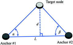

  

  Reference figure for Question 8

• 9. In this problem you will use MATLAB to simulate the APIT localization algorithm. Assume that the WSN occupies a 20 × 20 region which is divided into 400 cells that are each 1 × 1 units in dimension. Let the bottom left corner of the region have the coordinates (0,0) and the top right corner have the coordinates (20,20). Assume that the anchors at (0,0), (5,2) and (3,8) are connected to form a triangular region, just like the anchors at (10,10), (10,20), (15,10) and the anchors at (20,0), (15,5) and (15,0). Randomly generate 100 coordinates within this 20 × 20 region (assume the coordinates are integer numbers, i.e., each of the x and y coordinates are integer values between 0 and 20 inclusive). These coordinates represent the locations of the normal WSN nodes. For any five of these nodes that lie inside the triangles, use the APIT approach to find their locations. Compare the locations found by the algorithm to the actual locations of these nodes (compute the error as the Euclidian distance between the true locations and the computed locations and find the mean error over the five nodes). Rerun the APIT process when the WSN is segmented into cells that are 2 × 2 units in dimension and when they are cells that are 4 × 4 units in dimension. Comment on how the localization error varies in relation to the cell size (be sure to use the same 5 nodes in all three cases).

• 10. How many receiving localization nodes are enough for a successful implementation of a TDoA method?

• 11. What is the optimal configuration of receivers in TDoA? Please explain why.

• 12. Given four receivers in a plane that use RSSI method of localization, derive mathematically the optimal configuration of receivers. Simulate using MATLAB various scenarios and show that the solution found theoretically gives the best localization accuracy.

• 13. Describe how (6.11) can be used for localization by combining two different methods. Which method can be combined here? What is the trade-off in combining two methods versus using only one of the localization methods?

References

I. Amundson and X. Koustsoukos, “A Survey on Localization for Mobile Wireless Sensor Networks,” in MELT’09 Proceedings of the 2nd international conference on Mobile entity localization and tracking in GPS-less environments, 2009.
J. Bachrach and C. Taylor, “Localization in Sensor Networks,” in Handbook of Sensor Networks: Algorithms and Architectures, Hoboken, John Wiley & Sons, Inc., 2005.
N. Bulusu, J. Heidemann and D. Estrin, “GPS-less low-cost outdoor localization for very small devices,” IEEE Personal Communications, vol. 7, no. 5, pp. 28–34, 2000.
W.P. Chen, J. Hou and L. Sha, “Dynamic clustering for acoustic target tracking in wireless sensor networks,” IEEE Transactions on Mobile Computing, vol. 3, no. 3, pp. 258–271, 2004.
R. Fuller, “Tutorial on Location Determination by RF Means,” Proc. the 2 nd International Workshop on Mobile Entity Localization and Tracking in GPS-less Environments, MELT, Orlando, Florida, 2009.
T. He, C. Huang, B.M. Blum, J.A. Stankovic and T. Abdelzaher, “Range-free localization schemes for large scale sensor networks,” Proc. of the 9th International Conference on Mobile Computing and Networking, New York, 2003.
H.T. Kung and D. Vlah, “Efficient Location Tracking Using Sensor Networks,” Proc. of 2003 IEEE Wireless Communications, 2003.
B. Kusy, J. Sallai, G. Balogh, A. Ledeczi, V.-d. Protopopescu, J. Tolliver, F. DeNap and M. Parang, “Radio interferometric tracking of mobile wireless nodes,” Proc. of the 5th International Conference on Mobile Systems, Applications and Services, 2007.
E.D. Manley, H.A. Nahas and J.S. Deogun, “Localization and Tracking in Sensor Systems,” in Proc. Sensor Networks, Ubiquitous, and Trustworthy Computing, International Conference, 2006.
G. Mao, B. Fidan and B.D. Anderson, “Wireless Sensor Network Localization Techniques,” Computer Networks: The International Journal of Computer and Telecommunications Networking, vol. 51, no. 10, pp. 2529–2553, 2007.
D. Niculescu and B. Nath, “Ad hoc positioning system (APS) using AOA,” Proc. 22 nd Annual Joint Conference of the IEEE Computer and Communications, 2003.
A.T. Parameswaran, M.I. Husain and S. Upadhyaya, “Is RSSI a reliable parameter in sensor localization algorithms: An experimental study,” Field Failure Data Analysis Workshop, 2009.
M. R. Gholami, Positioning Algorithms for Wireless Sensor Networks, Gothenburg, Ph.D. Dissertation, Department of Signals and Systems, Chalmers University of Technology, 2011.
M. Rabbat and R. Nowak, “Distributed optimization in sensor networks,” Proc. the 3rd International Symposium on Information Processing in Sensor Networks, 2004.
F. Reichenbach, J. Salzmann, D. Timmermann, A. Born and R. Bill, “DLS: A Resource-Aware Localization Algorithm with High Precision in Large Wireless Sensor Networks,” Proc. 4 th Workshop on Positioning, Navigation and Communication, Hannover, 2007.
K. Römer, “The Lighthouse Location System for Smart Dust,” Proc. the 1 st International Conference on Mobile Systems, Applications and Services, 2003.
M.L. Sichitiu and V. Ramadurai, Localization of Wireless Sensor Networks with a Mobile Beacon, 3 ed., Technical Report TR-03/06, 2003, pp. 174–183.
J.O. Smith and J.S. Abel, “Closed-form least-squares source location estimation from range-difference measurements,” IEEE Transactions on Acoustics, Speech, and Signal Processing, vol. asp-35, no. 12, 1987.
R. Stoleru, T. He, J. A. Stankovic and D. Luebke, “A high-accuracy, low-cost localization system for wireless sensor networks,” Proc. the 3rd International Conference on Embedded Networked Sensor Systems, 2005.
J.B. Tenenbaum, V.d. Silva and J.C. Langford, “A Global Geometric Framework for Nonlinear Dimensionality Reduction,” Science, vol. 290, p. 2319, 2000.
Y. Xu and W.-C. Lee, “On localized prediction for power efficient object tracking in sensor networks,” Proc. 23 rd International Conference on Distributed Computing Systems Workshops, 2003.
N. Xu, S. Rangwala, K.K. Chintalapudi, D. Ganesan, A. Broad, R. Govindan and D. Estrin, “A wireless sensor network for structural monitoring,” Proc. of the 2nd International Conference on Embedded Networked Sensor Systems, 2004.
Y. Xu, W. J. and W.-C. Lee, “Prediction-based strategies for energy saving in object tracking sensor networks,” Proc. International Conference in Mobile Data Management, 2004.
Y. Xu, W. J. and W.-C. Lee, “Dual prediction-based reporting for object tracking sensor networks,” Proc. of the 1 st International Conference on Mobile and Ubiquitous Systems: Networking and Services, 2004.
H. Yang and B. Sikdar, “A protocol for tracking mobile targets using sensor networks,” Proc. of the 1 st IEEE International Workshop in Sensor Network Protocols and Applications, 2003.
W. Zhang and G. Cao, “DCTC: dynamic convoy tree-based collaboration for target tracking in sensor networks,” IEEE Transactions on Wireless Communications, vol. 3, no. 5, pp. 1689–1701, 2004.
Z. Zhong, Range-Free Localization and Tracking in Wireless Sensor Networks, Ph.D. Dissertation, University of Minnesota, 2010.
Z. Zhou, J.-H. Cui and S. Zhou, “Localization for Large-Scale Underwater Sensor Networks,” UCONN CSE Technical Report: UbiNet-TR06-04, 2006.
Author information
Authors and Affiliations
Corresponding author