Colliding Bodies Optimization

Abstract

This chapter presents a novel efficient metaheuristic optimization algorithm called colliding bodies optimization (CBO) for optimization. This algorithm is based on one-dimensional collisions between bodies, with each agent solution being considered as the massed object or body. After a collision of two moving bodies having specified masses and velocities, these bodies are separated with new velocities. This collision causes the agents to move toward better positions in the search space. CBO utilizes a simple formulation to find minimum or maximum of functions; also it is independent of parameters [1].

These keywords were added by machine and not by the authors. This process is experimental and the keywords may be updated as the learning algorithm improves.

7.1 Introduction

This chapter presents a novel efficient metaheuristic optimization algorithm called colliding bodies optimization (CBO) for optimization. This algorithm is based on one-dimensional collisions between bodies, with each agent solution being considered as the massed object or body. After a collision of two moving bodies having specified masses and velocities, these bodies are separated with new velocities. This collision causes the agents to move toward better positions in the search space. CBO utilizes a simple formulation to find minimum or maximum of functions; also it is independent of parameters [1].

This chapter consists of two parts. In the first part the main algorithm is developed, and three well-studied engineering design problems and two structural design problems taken from the optimization literature are used to investigate the efficiency of the proposed approach [1]. In the second part, the CBO is applied to a number of continuous optimization benchmark problems. These examples include three well-studied space trusses and two planar bridge structures [2].

7.2 Colliding Bodies Optimization

The main goal of this section is to introduce a simple optimization algorithm based on the collision between objects, which is called colliding bodies optimization (CBO).

7.2.1 The Collision Between Two Bodies

Collisions between bodies are governed by the laws of momentum and energy. When a collision occurs in an isolated system (Fig. 7.1), the total momentum of the system of objects is conserved. Provided that there are no net external forces acting upon the objects, the momentum of all objects before the collision equals the momentum of all objects after the collision.

Fig. 7.1

The collision between two bodies. (a) Before the collision and (b) after the collision [1]

The conservation of the total momentum demands that the total momentum before the collision is the same as the total momentum after the collision and can be expressed by the following equation:

$$ {m}_1{v}_1+{m}_2{v}_2={m}_1{v}_1^{\hbox{'}}+{m}_2{v}_2^{\hbox{'}} $$

(7.1)

Likewise, the conservation of the total kinetic energy is expressed as:

$$ \frac{1}{2}{m}_1{v_1}^2+\frac{1}{2}{m}_2{v_2}^2=\frac{1}{2}{m}_1{v_1^{\hbox{'}}}^2+\frac{1}{2}{m}_2{v_2^{\hbox{'}}}^2+Q $$

(7.2)

where v ₁ is the initial velocity of the first object before impact, v ₂ is the initial velocity of the second object before impact, v ^'₁ is the final velocity of the first object after impact, v ^'₂ is the final velocity of the second object after impact, m ₁ is the mass of the first object, m ₂ is the mass of the second object, and Q is the loss of kinetic energy due to the impact [3].

The formulas for the velocities after a one-dimensional collision are:

$$ {v}_1^{\hbox{'}}=\frac{\left({m}_1-\varepsilon {m}_2\right){v}_1+\left({m}_2+\varepsilon {m}_2\right){v}_2}{m_1+{m}_2} $$

(7.3)

$$ {v}_2^{\hbox{'}}=\frac{\left({m}_2-\varepsilon {m}_1\right){v}_2+\left({m}_1+\varepsilon {m}_1\right){v}_1}{m_1+{m}_2} $$

(7.4)

where ε is the coefficient of restitution (COR) of the two colliding bodies, defined as the ratio of relative velocity of separation to relative velocity of approach:

$$ \varepsilon =\frac{\left|{v}_2^{\hbox{'}}-{v}_1^{\hbox{'}}\right|}{\left|{v}_2-{v}_1\right|}=\frac{v^{\hbox{'}}}{v} $$

(7.5)

According to the coefficient of restitution, there are two special cases of any collision as follows:

• 1) A perfectly elastic collision is defined as the one in which there is no loss of kinetic energy in the collision ($\begin{array}{ccc}\hfill Q=0\hfill & \hfill and\hfill & \hfill \varepsilon =1\hfill \end{array}$). In reality, any macroscopic collision between objects will convert some kinetic energy to internal energy and other forms of energy. In this case, after collision, the velocity of separation is high.

• 2) An inelastic collision is the one in which part of the kinetic energy is changed to some other forms of energy in the collision. Momentum is conserved in inelastic collisions (as it is for elastic collisions), but one cannot track the kinetic energy through the collision since some of it will be converted to other forms of energy. In this case, coefficient of restitution does not equal to one ($\begin{array}{ccc}\hfill Q\ne 0\hfill & \hfill \&\hfill & \hfill \varepsilon \le 1\hfill \end{array}$). In this case, after collision the velocity of separation is low.

For the most real objects, the value of ε is between 0 and 1.

7.2.2 The CBO Algorithm

7.2.2.1 Theory

The main objective of the present study is to formulate a new simple and efficient metaheuristic algorithm which is called colliding bodies optimization (CBO). In CBO, each solution candidate X _i containing a number of variables (i.e., ${X}_i=\left\{{X}_{i,j}\right\}$) is considered as a colliding body (CB). The massed objects are composed of two main equal groups, i.e., stationary and moving objects, where the moving objects move to follow stationary objects and a collision occurs between pairs of objects. This is done for two purposes: (i) to improve the positions of moving objects and (ii) to push stationary objects toward better positions. After the collision, new positions of colliding bodies are updated based on new velocity by using the collision laws as discussed in the following:

The CBO procedure can briefly be outlined as

• 1. The initial positions of CBs are determined with random initialization of a population of individuals in the search space:

  $$ {x}_i^0={x}_{\min }+ rand\left({x}_{\max }-{x}_{\min}\right)\begin{array}{cc}\hfill, \hfill & \hfill i=1,2,\dots, n\hfill \end{array}, $$

  (7.6)

  where x ⁰ _i determines the initial value vector of the ith CB, x _min and x _max are the minimum and the maximum allowable value vectors of variables, rand is a random number in the interval [0,1], and n is the number of CBs.

• 2. The magnitude of the body mass for each CB is defined as:

  $$ {m}_k=\frac{\frac{1}{fit(k)}}{\sum_{i=1}^n\frac{1}{fit(i)}}\begin{array}{cc}\hfill, \hfill & \hfill k=1,2,\dots, n\hfill \end{array} $$

  (7.7)

  where fit(i ) represents the objective function value of the agent i and n is the population size. It seems that a CB with good values exerts a larger mass than the bad ones. Also, for maximization, the objective function fit(i ) will be replaced by $\frac{1}{fit(i)}$.

• 3. The arrangement of the CBs objective function values is performed in ascending order (Fig. 7.2a). The sorted CBs are equally divided into two groups:

  • The lower half of CBs (stationary CBs); These CBs are good agents which are stationary, and the velocity of these bodies before collision is zero. Thus:

    $$ {v}_i=0\begin{array}{cc}\hfill, \hfill & \hfill i=1,\dots, \frac{n}{2}\hfill \end{array} $$

    (7.8)

  • The upper half of CBs (moving CBs): These CBs move toward the lower half. Then, according to Fig. 7.2b, the better and worse CBs, i.e., agents with upper fitness value, of each group will collide together. The change of the body position represents the velocity of these bodies before collision as:

    $$ {v}_i={x}_i-{x}_{i-\frac{n}{2}},\begin{array}{cc}\hfill \hfill & \hfill i=\frac{n}{2}+1,\dots, n\hfill \end{array} $$

    (7.9)

    where v _i and x _i are the velocity and position vector of the ith CB in this group, respectively, and ${x}_{i-\frac{n}{2}}$ is the ith CB pair position of x _i in the previous group.

  Fig. 7.2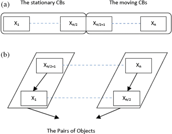

  

  (a) CBs sorted in increasing order; (b) colliding object pairs [1]

• 4. After the collision, the velocities of the colliding bodies in each group are evaluated utilizing Eqs. (7.3) and (7.4) and the velocity before collision. The velocity of each moving CBs after the collision is obtained by:

  $$ {v}_i^{\hbox{'}}=\frac{\left({m}_i-\varepsilon {m}_{i-\frac{n}{2}}\right){v}_i}{m_i+{m}_{i-\frac{n}{2}}}\begin{array}{cc}\hfill, \hfill & \hfill i=\frac{n}{2}+1,\dots, n\hfill \end{array} $$

  (7.10)

  where v _i and v ^' _i are the velocity of the ith moving CB before and after the collision, respectively; m _i is the mass of the ith CB; and ${m}_{i-\frac{n}{2}}$ is the mass of the ith CB pair. Also, the velocity of each stationary CB after the collision is:

  $$ {v}_i^{\hbox{'}}=\frac{\left({m}_{i+\frac{n}{2}}+\varepsilon {m}_{i+\frac{n}{2}}\right){v}_{i+\frac{n}{2}}}{m_i+{m}_{i+\frac{n}{2}}}\begin{array}{cc}\hfill, \hfill & \hfill i=1,\dots, \frac{n}{2}\hfill \end{array} $$

  (7.11)

  where ${v}_{i+\frac{n}{2}}$ and v ^' _i are the velocity of the ith moving CB pair before and the ith stationary CB after the collision, respectively; m _i is the mass of the ith CB; ${m}_{i+\frac{n}{2}}$ is the mass of the ith moving CB pair; and ε is the value of the COR parameter whose law of variation will be discussed in the next section.

• 5. New positions of CBs are evaluated using the generated velocities after the collision in position of stationary CBs.

  The new positions of each moving CB are:

  $$ {x}_i^{new}={x}_{i-\frac{n}{2}}+ rand\circ {v}_i^{\hbox{'}}\begin{array}{cc}\hfill, \hfill & \hfill i=\frac{n}{2}+1,\dots, n\hfill \end{array} $$

  (7.12)

  where x ^new _i and v ^' _i are the new position and the velocity after the collision of the ith moving CB, respectively, and ${x}_{i-\frac{n}{2}}$ is the old position of the stationary CB pair. Also, the new positions of stationary CBs are obtained by:

  $$ {x}_i^{new}={x}_i+ rand\circ {v}_i^{\hbox{'}}\begin{array}{cc}\hfill, \hfill & \hfill i=1,\dots, \frac{n}{2}\hfill \end{array} $$

  (7.13)

  where x ^new _i , x _i , and v ^' _i are the new position, the old position, and the velocity after the collision of the ith stationary CB, respectively; rand is a random vector uniformly distributed in the range (−1,1); and the sign “$\circ$” denotes an element-by-element multiplication.

• 6. The optimization is repeated from Step 2 until a termination criterion, such as maximum iteration number, is satisfied. It should be noted that a body’s status (stationary or moving body) and its numbering are changed in two subsequent iterations.

Apart from the efficiency of the CBO algorithm, which is illustrated in the next section through numerical examples, parameter independency is an important feature that makes CBO superior over other metaheuristic algorithms. Also, the formulation of CBO algorithm does not use the memory which saves the best-so-far solution (i.e., the best position of agents from the previous iterations).

The penalty function approach was used for constraint handling. The fit(i) function corresponds to the effective cost. If optimization constraints are satisfied, there is no penalty; otherwise, the value of penalty is calculated as the ratio between the violation and the allowable limit.

7.2.2.2 The Coefficient of Restitution (COR)

The metaheuristic algorithms have two phases: exploration of the search space and exploitation of the best solutions found. In the metaheuristic algorithm, it is very important to have a suitable balance between the exploration and exploitation. In the optimization process, the exploration should be decreased gradually, while simultaneously exploitation should be increased.

In this chapter, an index is introduced in terms of the coefficient of restitution (COR) to control exploration and exploitation rate. In fact, this index is defined as the ratio of the separation velocity of two agents after collision to approach velocity of two agents before collision. Efficiency of this index will be shown using one numerical example.

In this section, in order to have a general idea about the performance of COR in controlling local and global searches, a benchmark function (Aluffi-Pentini) chosen from Ref. [4] is optimized using the CBO algorithm. Three variants of COR values are considered. Figure 7.3 is prepared to show the positions of the current CBs in the 1st, 50th, and 100th iteration for these cases. These three typical cases result in the following:

Fig. 7.3

Evolution of the positions of CBs during optimization history for different definitions of the coefficient of restitution (Aluffi-Pentini benchmark function) [1]

• 1. The perfectly elastic collision: In this case, COR is set equal to unity. It can be seen that in the final iterations, the CBs investigate the entire search space to discover a favorite space (global search).

• 2. The hypothetical collision: In this case, COR is set equal to zero. It can be seen that in the 50th iterations, the movements of the CBs are limited to very small space in order to provide exploitation (local search). Consequently, the CBs are gathered in a small region of the search space.

• 3. The inelastic collision: In this case, COR decreases linearly to zero and ε is defined as:

  $$ \varepsilon =1-\frac{iter}{ite{r}_{\max }} $$

  (7.14)

  where iter is the actual iteration number and iter _max is the maximum number of iterations. It can be seen that the CBs get closer by increasing iteration. In this way a good balance between the global and local search is achieved. Therefore, in the optimization process, COR is considered such as the above equation.

7.2.3 Test Problems and Optimization Results

Three well-studied engineering design problems and two structural design problems taken from the optimization literature are used to investigate the efficiency of the proposed approach. These examples have been previously studied using a variety of other techniques, which are useful to show the validity and effectiveness of the proposed algorithm. In order to assess the effect of the initial population on the final result, these examples are independently optimized with different initial populations.

For engineering design examples, 30 independent runs were performed for CBO, considering 20 individuals and 200 iterations; the corresponding number of function evaluations is 4000. The number of function evaluations set for the GA-based algorithm developed by Coello [5], the PSO-based method developed by He and Wang [6], and the evolution strategies developed by Montes and Coello [7] are 900,000, 200,000, and 25,000, respectively. Similar to CBO, the number of function evaluations for the charged system search algorithm developed by Kaveh and Talatahari [8] is 4000.

In the truss design problems, 20 independent runs were carried out, considering 40 individuals and 400 iterations; hence, the maximum number of structural analyses was 16,000. The CBO algorithm was coded in MATLAB. Structural analysis was performed with the direct stiffness method.

7.2.3.1 Example 1: Design of Welded Beam

As the first example, design optimization of the welded beam shown in Fig. 7.4 is carried out. The welded beam design problem was often utilized to evaluate the performance of different optimization methods. The objective is to find the best set of design variables to minimize the total fabrication cost of the structure subject to shear stress (τ), bending stress (σ), buckling load (Pc), and end deflection (δ) constraints. Assuming x ₁ = h, x ₂ = l, x ₃ = t, and x ₄ = b as the design variables, the mathematical formulation of the problem can be expressed as:

Fig. 7.4

Schematic of the welded beam structure with indication of design variables

Find

$$ \left\{{x}_1,{x}_2,{x}_3,{x}_4\right\} $$

(7.15)

To minimize

$$ \begin{array}{cc}\hfill \hfill & \hfill \cos t(x)=1.10471{x}_1^2{x}_2+0.04811{x}_3{x}_4\left(14+{x}_2\right)\hfill \end{array} $$

(7.16)

Subjected to

$$ \begin{array}{c}\hfill {g}_1(x)=\tau (x)-{\tau}_{\max}\le 0\hfill \\ {}\hfill {g}_2(x)=\sigma (x)-{\sigma}_{\max}\le 0\hfill \\ {}\hfill {g}_3(x)={x}_1-{x}_4\le 0\hfill \\ {}\hfill {g}_4(x)=0.10471{x}_1^2+0.04811{x}_3{x}_4\left(14+{x}_2\right)-5\le 0\hfill \\ {}\hfill {g}_5(x)=0.125-{x}_1\le 0\hfill \\ {}\hfill {g}_6(x)=\delta (x)-{\delta}_{\max}\le 0\hfill \\ {}\hfill {g}_7(x)=p-{p}_c(x)\le 0\hfill \end{array} $$

(7.17)

The bounds on the design variables are:

$$ \begin{array}{cccc}\hfill 0.1\le {x}_1\le 2,\hfill & \hfill 0.1\le {x}_2\le 10,\hfill & \hfill 0.1\le {x}_3\le 10,\hfill & \hfill 0.1\le {x}_4\le 2\hfill \end{array} $$

(7.18)

where

$$ \begin{array}{l}\begin{array}{l}\tau (x)=\sqrt{{\left({\tau}^{\hbox{'}}\right)}^2+2{\tau}^{\hbox{'}}{\tau}^{\hbox{'}\hbox{'}}\frac{x_2}{2R}+{\left({\tau}^{\hbox{'}\hbox{'}}\right)}^2}\hfill \\ {}{\tau}^{\hbox{'}}=\frac{P}{\sqrt{2}{x}_1{x}_2}{\tau}^{\hbox{'}\hbox{'}}=\frac{MR}{J}M=P\left(L+\frac{x_2}{2}\right)R=\sqrt{\frac{x_2^2}{4}+{\left(\frac{x_1+{x}_3}{2}\right)}^2}\hfill \\ {}J=2\left\{\sqrt{2}{x}_1{x}_2\left[\frac{x_2^2}{12}+{\left(\frac{x_1+{x}_3}{2}\right)}^2\right]\right\}\sigma (x)=\frac{6 PL}{x_4{x}_3^2}\delta (x)=\frac{4P{L}^3}{E{x}_3^3{x}_4}\hfill \end{array}\hfill \\ {}{P}_c(x)=\frac{4.013\sqrt{E\left({x}_3^2{x}_4^6/36\right)}}{L^2}\left(1-\frac{x_3}{2L}\sqrt{\frac{E}{4G}}\right)\hfill \end{array} $$

(7.19)

The constants in Eqs. (7.17) and (7.19) are chosen as follows:

• P = 6000 lb, L = 14 in., E = 30 × 106 psi, G = 12 × 106 psi, τ_max = 13,600 psi, σ_max = 30,000 psi, and δ_max = 0.25 in.

Radgsdell and Phillips [9] compared optimal results of different optimization methods which were mainly based on mathematical optimization algorithms. Deb [10], Coello [5], and Coello and Montes [11] solved this problem using GA-based methods. Also, He and Wang [6] used effective coevolutionary particle swarm optimization, Montes and Coello [7] solved this problem utilizing evolution strategies, and Kaveh and Talatahari [8] employed charged system search.

Table 7.1 compares the optimized design and the corresponding cost obtained by CBO with those obtained by other metaheuristic algorithms documented in literature. It can be seen that the best solution obtained by CBO is better than those quoted for the other algorithms. The statistical data on 30 independent runs reported in Table 7.2 also demonstrate the better search ability of CBO with respect to the other algorithms: in fact the best, worst, and average costs and the standard deviation (SD) of the obtained solutions are better than literature. The lowest standard deviation achieved by CBO proves that the present algorithm is more robust than other metaheuristic methods.

Table 7.1 Comparison of CBO optimized designs with literature for the welded beam problem

Table 7.2 Statistical results from different optimization methods for the welded beam design problem

7.2.3.2 Test Problem 2: Design of a Pressure Vessel

Design optimization of the cylindrical pressure vessel capped at both ends by hemispherical heads (Fig. 7.5) is considered as the second example. The objective of optimization is to minimize the total manufacturing cost of the vessel based on the combination of welding, material, and forming costs. The vessel is designed for a working pressure of 3000 psi and a minimum volume of 750 ft³ regarding the provisions of ASME boiler and pressure vessel code. Here, the shell and head thicknesses should be multiples of 0.0625 in. The thickness of the shell and head is restricted to 2 in. The shell and head thicknesses must not be <1.1 in. and 0.6 in., respectively. The design variables of the problem are x ₁ as the shell thickness (T _s ), x ₂ as the spherical head thickness (T _h ), x ₃ as the radius of cylindrical shell (R), and x ₄ as the shell length (L ). The problem formulation is as follows:

Fig. 7.5

Schematic of the spherical head and cylindrical wall of the pressure vessel with indication of design variables

Find

$$ \left\{{x}_1,{x}_2,{x}_3,{x}_4\right\} $$

(7.20)

To minimize

$$ \begin{array}{cc}\hfill \hfill & \hfill \cos t(x)=0.6224{x}_3{x}_1{x}_4+1.7781{x}_3^2{x}_2+3.1611{x}_1^2{x}_4+19.8621{x}_3{x}_1^2\hfill \end{array} $$

(7.21)

Subject to

$$ \begin{array}{c}\hfill {g}_1(x)=0.0193{x}_3-{x}_1\le 0\hfill \\ {}\hfill {g}_2(x)=0.00954{x}_3-{x}_2\le 0\hfill \\ {}\hfill {g}_3(x)=750\times 1728-\pi {x}_3^2{x}_4-\frac{4}{3}\pi {x}_3^3\le 0\hfill \\ {}\hfill {g}_4(x)={x}_4-240\le 0\hfill \end{array} $$

(7.22)

The bounds on the design variables are:

$$ \begin{array}{cccc}\hfill 1.125\le {x}_1\le 2,\hfill & \hfill 0.625\le {x}_2\le 2,\hfill & \hfill 10\le {x}_3\le 240,\hfill & \hfill 10\le {x}_4\le 240\hfill \end{array} $$

(7.23)

It can be seen in Table 7.3 that the present algorithm found the best design overall which is about 3 % lighter than the best known design quoted in literature (5889.911 versus 6059.088 of Ref. [8]). The statistical data reported in Table 7.4 indicate that the standard deviation of CBO optimized solutions is the third lowest among those quoted for the different algorithms compared in this test case. Statistical results given in Table 7.4 indicate that CBO is in general more robust than the other metaheuristic algorithms. However, the worst optimized design and standard deviation found by CBO are higher than for CSS.

Table 7.3 Comparison of CBO optimized designs with literature for the pressure vessel problem

Table 7.4 Statistical results from different optimization methods for the pressure vessel problem

7.2.3.3 Test Problem 3: Design of a Tension/Compression Spring

This problem was first described by Belegundu [15] and Arora [16]. It consists of minimizing the weight of a tension/compression spring subject to constraints on shear stress, surge frequency, and minimum deflection as shown in Fig. 7.6. The design variables are the wire diameter d (=x ₁), the mean coil diameter D (=x ₂), and the number of active coils N (=x ₃). The problem can be stated as follows:

Fig. 7.6

Schematic of the tension/compression spring with indication of design variables

Find

$$ \left\{{x}_1,{x}_2,{x}_3\right\} $$

(7.24)

To minimize

$$ \begin{array}{cc}\hfill \hfill & \hfill \cos t(x)=\left({x}_3+2\right){x}_2{x}_1^2\hfill \end{array} $$

(7.25)

Subject to

$$ \begin{array}{c}\hfill {g}_1(x)=1-\frac{x_2^3{x}_3}{71785{x}_1^4}\le 0\hfill \\ {}\hfill {g}_2(x)=\frac{4{x}_2^2-{x}_1{x}_2}{12566\left({x}_2{x}_1^3-{x}_1^4\right)}+\frac{1}{5108{x}_1^2}-1\le 0\hfill \\ {}\hfill {g}_3(x)=1-\frac{140.45{x}_1}{x_2^2{x}_3}\le 0\hfill \\ {}\hfill {g}_4(x)=\frac{x_1+{x}_2}{1.5}-1\le 0\hfill \end{array} $$

(7.26)

The bounds on the design variables are:

$$ \begin{array}{cccc}\hfill 0.05\le {x}_1\le 2,\hfill & \hfill 0.25\le {x}_2\le 1.3,\hfill & \hfill 2\le {x}_3\le 15,\hfill & \hfill \hfill \end{array} $$

(7.27)

This problem has been solved by Belegundu [15] using eight different mathematical optimization techniques. Arora [16] also solved this problem using a numerical optimization technique called a constraint correction at the constant cost. Coello [5] as well as Coello and Montes [11] solved this problem using GA-based method. Additionally, He and Wang [6] utilized a co-evolutionary particle swarm optimization (CPSO). Recently, Montes and Coello [7] and Kaveh and Talatahari [8] used evolution strategies and the CSS to solve this problem, respectively.

Tables 7.5 and 7.6 compare the best results obtained in this chapter and those of the other researches. Once again, CBO found the best design overall. In fact, the lighter design found by Kaveh and Talatahari in [8] actually violates the first two optimization constraints. The statistical data reported in Table 7.6 show that the standard deviation on optimized cost seen for CBO is fully consistent with literature.

Table 7.5 Comparison of CBO optimized designs with literature for the tension/compression spring problem

Table 7.6 Statistical results from different optimization methods for tension/compression string problem

7.2.3.4 Test Problem 4: Weight Minimization of the 120-Bar Truss Dome

The fourth test case solved in this study is the weight minimization problem of the 120-bar truss dome shown in Fig. 7.7. This test case was investigated by Soh and Yang [17] as a configuration optimization problem. It has been solved later as a sizing optimization problem by Lee and Geem [18], Kaveh and Talatahari [8], and Kaveh and Khayatazad [19].

Fig. 7.7

Schematic of the spatial 120-bar dome truss with indication of design variables and main geometric dimensions

The allowable tensile and compressive stresses are set according to the ASD-AISC (1989) [20] code, as follows:

$$ \left\{\begin{array}{c}\hfill {\sigma}_i^{+}=0.6{F}_y\begin{array}{cc}\hfill \hfill & \hfill for{\sigma}_i\ge 0\hfill \end{array}\hfill \\ {}\hfill {\sigma}_i^{-}\begin{array}{cc}\hfill \begin{array}{cc}\hfill \begin{array}{cc}\hfill \hfill & \hfill \hfill \end{array}\hfill & \hfill \hfill \end{array}\hfill & \hfill for{\sigma}_i\le 0\hfill \end{array}\hfill \end{array}\right. $$

(7.28)

where ${\sigma}_i^{-}$ is calculated according to the slenderness ratio

$$ {\sigma}_i^{-}=\left\{\begin{array}{c}\hfill \left[\left(1-\frac{\lambda_i^2}{2{C}_c^2}\right){F}_y\right]/\left(\frac{5}{3}+\frac{3{\lambda}_i}{8{C}_c}-\frac{\lambda_i^3}{8{C}_c^3}\right)\begin{array}{cc}\hfill \hfill & \hfill for{\lambda}_i<{C}_c\hfill \end{array}\hfill \\ {}\hfill \frac{12{\pi}^2E}{23{\lambda}_i^2}\begin{array}{cccc}\hfill \begin{array}{ccc}\hfill \begin{array}{cccc}\hfill \hfill & \hfill \hfill & \hfill \hfill & \hfill \hfill \end{array}\hfill & \hfill \hfill & \hfill \hfill \end{array}\hfill & \hfill \hfill & \hfill \hfill & \hfill for{\lambda}_i\ge {C}_c\hfill \end{array}\hfill \end{array}\right. $$

(7.29)

where E is the modulus of elasticity, F _y is the yield stress of steel, C _c is the slenderness ratio (λ _i ) dividing the elastic and inelastic buckling regions $\left({C}_c=\sqrt{2{\pi}^2E/{F}_y}\right)$ , λ _i is the slenderness ratio $\left({\lambda}_i=\frac{K{L}_i}{r_i}\right)$, K is the effective length factor, L _i is the member length, and r _i is the radius of gyration.

The modulus of elasticity is 30,450 ksi (210,000 MPa) and the material density is 0.288 lb/in³ (7971.810 kg/m³). The yield stress of steel is taken as 58.0 ksi (400 MPa). On the other hand, the radius of gyration (r _i ) is expressed in terms of cross-sectional areas as ${r}_i= aA{}_i{}^b$ [28]. Here, a and b are constants depending on the types of sections adopted for the members such as pipes, angles, and tees. In this example, pipe sections (a = 0.4993 and b = 0.6777) are adopted for bars. All members of the dome are divided into seven groups, as shown in Fig. 7.7. The dome is considered to be subjected to vertical loads at all the unsupported joints. These are taken as −13.49 kips (60 kN) at node 1, −6.744 kips (30 kN) at nodes 2 through 14, and −2.248 kips (10 kN) at the remaining of the nodes. The minimum cross-sectional area of elements is 0.775 in² (cm²). In this example, four cases of constraints are considered: with stress constraints and no displacement constraints (Case 1), with stress constraints and displacement limitations of ±0.1969 in (5 mm) imposed on all nodes in x and y directions (Case 2), no stress constraints but displacement limitations of ±0.1969 in (5 mm) imposed on all nodes in z directions (Case 3), and all constraints explained above (Case 4). For Case 1 and Case 2, the maximum cross-sectional area is 5.0 in² (32.26 cm²) while for Case 3 and Case 4 is 20.0 in² (129.03 cm²).

Table 7.7 compares the optimization results obtained in this study with previous research presented in literature. It can be seen that CBO always designed the lightest structure except for Cases 3 and 4 where HPSACO converged to a slightly lower weight. CBO always completed the optimization process within 16,000 structural analyses (40 agents × 400 optimization iterations), while HPSACO required on average 10,000 analyses (400 optimization iterations) and PSOPC required 125,000 analyses (2500 iterations). The average number of analyses required by the RO algorithm was instead 19,900. Figure 7.8 shows that the convergence rate of CBO is considerably higher than that of PSO and PSOPC.

Table 7.7 Comparison of CBO optimized designs with literature in the 120-bar dome problem

Fig. 7.8

Convergence curves obtained for the different variants of the 120-bar dome problem [2]

7.2.3.5 Test Problem 5: Design of Forth Truss Bridge

The last test case was the layout optimization of the Forth Bridge shown in Fig. 7.9a which is a 16 m long and 1 m high truss of infinite span. Because of infinite span, the cross section of the bridge can be modeled as symmetric about the axis joining nodes 10 and 11. Structural symmetry allowed the 37 elements of which the bridge is comprised to be grouped into 16 groups (see Table 7.8); hence, there are 16 independent sizing variables. Nodal coordinates were included as layout variables: x-coordinates of nodes could not vary, while y-coordinates (except those of nodes 1 and 20) were allowed to change between −140 and 140 cm with respect to the initial configuration of Fig. 7.9a. Thus, the optimization problem included also ten layout variables. The cross-sectional areas (sizing variables) could vary between 0.5 and 100 cm².

Fig. 7.9

(a) Schematic of the Forth Truss Bridge, (b) optimized layout of the Forth Bridge [2]

Table 7.8 Comparison of CBO optimization results with literature for the Forth Bridge problem

Material properties were set as follows: modulus of elasticity of 210 GPa, allowable stress of 250 MPa, and specific weight of 7.8 t/m³. The structure is subject to self-weight and concentrated loads shown in Fig. 7.9a.

Table 7.8 compares CBO optimization results with literature. It appears that CBO found the best design overall saving about 1000 kg with respect to the optimum currently reported in literature. Furthermore, the standard deviation on optimized weight observed for CBO in 20 independent optimization runs was lower than for the other metaheuristic optimization algorithms taken as basis of comparison.

The optimized layout of the bridge is shown in Fig. 7.9b. Figure 7.10 compares the convergence behavior of CBO and RO. Although RO was considerably faster in the early optimization iterations, CBO converged to a significantly better design without being trapped in local optima.

Fig. 7.10

Convergence curves obtained in the Forth Bridge problem [2]

7.3 CBO for Optimum Design of Truss Structures with Continuous Variables

This part considers the following: (i) The CBO algorithm is introduced for optimization of continuous problems. (ii) A comprehensive study of sizing optimization for truss structures is presented. The examples are chosen from the literature to verify the effectiveness of the algorithm. These examples are as follows: a 25-member spatial truss with 8 design variables, a 72-member spatial truss with 16 design variables, a 582-member space truss tower with 32 design variables, a 37-member plane truss bridge with 16 design variables, and a 68-member plane truss bridge with 4, 8, and 12 design variables. All the structures are optimized for minimum weight with CBO algorithm, and a comparison is carried out in terms of the best optimum solutions and their convergence rates in a predefined number of analyses. The results indicate that the proposed algorithm is very competitive with other state-of-the-art metaheuristic methods.

7.3.1 Flowchart and CBO Algorithm

The flowchart of the CBO algorithm is shown in Fig. 7.11. The main steps of CBO algorithm are as follows:

Fig. 7.11

The flowchart of the CBO [2]

Level 1: Initialization

• Step 1: Initialization. Initialize an array of CBs with random positions and their associated values of the objective function [Eq. (7.6)].

Level 2: Search

• Step 1: CBs ranking. Compare the value of the objective function for each CB, and sort them in an increasing order.

• Step 2: Group creation. CBs are divided into two equal groups: (i) stationary group and (ii) moving group. Then, the pairs of CB are defined for collision (Fig. 7.2).

• Step 3: Criteria before the collision. The value of mass and velocity of each CB for each group is evaluated before the collision [Eqs. (7.7)–(7.9)].

• Step 4: Criteria after the collision. The value velocity of each CB in each groups is evaluated after the collision [Eqs. (7.10) and (7.11)].

• Step 5: CBs updating. The new position of each CB is calculated [Eqs. (7.13) and Eq. (7.14)].

Level 3: Terminating Criterion Control

• Step 1: Repeat search level steps until a terminating criterion is satisfied.

7.3.2 Numerical Examples

In order to assess the effectiveness of the proposed methodology, a number of continuous optimization benchmark problems are examined. These examples include three well-known space trusses and two planar bridge structures. The numbers of design variables for the first to fifth examples are 8, 16, 32, and 26, respectively, and for the last example, 4, 8, and 12 variables are used. Similarly, the numbers of colliding bodies or agents for these examples are considered as 30, 40, 50, 40, and 20, respectively. For all of these examples, the maximum number of iteration is considered as 400. The algorithm and the direct stiffness method for the analysis of truss structures are coded in MATLAB software.

For the sake of simplicity and to be fair in comparisons, the penalty approach is used for the constraint handling. The constrained objective function can formally be stated as follows:

$$ Mer(X)=f(X)\times {f}_{penalty}(X)=f(X)\times {\left(1+{\varepsilon}_1{\displaystyle \sum_{i=1}^{ni} \max \left(0,{g}_i(x)\right)}\right)}^{\varepsilon_2} $$

(7.30)

where X is the vector of design variables, g _i is the ith constraint from n _i inequality constraints (g _i (X ) ≤ 0, i = 1, 2, …, n _i ), Mer(X ) is the merit function, f(X ) is the weight of structure, and f _penalty (X ) is the penalty function which results from the violations of the constraints corresponding to the response of the structure. The parameters ε ₁ and ε ₂ are selected considering the exploration and the exploitation rate of the search space. In this study, ε ₁ is selected as unity and ε ₂ is taken as 1.5 at the start and linearly increases to 6.

7.3.2.1 A 25-Bar Spatial Truss

Size optimization of the 25-bar planar truss shown in Fig. 7.12 is considered. This is a well-known problem in the field of weight optimization of the structures. In this example, the material density is considered as 0.1 lb/in³ (2767.990 kg/m³), and the modulus of elasticity is taken as 10,000 ksi (68,950 MPa). Table 7.9 shows the two load cases for this example. The structure includes 25 members, which are divided into eight groups, as follows: (1) A₁, (2) A₂–A₅, (3) A₆–A₉, (4) A₁₀–A₁₁, (5) A₁₂–A₁₃, (6) A₁₄–A₁₇, (7) A₁₈–A₂₁, and (8) A₂₂–A₂₅.

Fig. 7.12

Schematic of a 25-bar spatial truss

Table 7.9 Loading conditions for the 25-bar spatial truss

Maximum displacement limitations of ±0.35 in (8.89 mm) are imposed on every node in every direction, and the axial stress constraints vary for each group as shown in Table 7.10. The range of the cross-sectional areas varies from 0.01 to 3.4 in² (0.6452–21.94 cm²).

Table 7.10 Member stress limitations for the 25-bar spatial truss

By the use of the proposed algorithm, this optimization problem is solved, and Table 7.11 shows the obtained optimal design of CBO, which is compared with GA [21], PSO [22], HS [6], and RO [19]. The best weight of the CBO is 544.310 lb, which is slightly improved compared to other algorithms. It is evident in Table 7.11 that the number of analyses and standard deviation of 20 independent runs for the CBO are 9090 and 0.294 lb, respectively, which are much less than the other optimization algorithms. Figure 7.13 provides the convergence diagram of the CBO in 400 iterations.

Table 7.11 Comparison of CBO optimized designs with literature in the 25-bar spatial truss

Fig. 7.13

The convergence diagram for the 25-bar spatial truss [2]

7.3.2.2 A 72-Bar Spatial Truss Structure

Schematic topology and element numbering of a 72-bar space truss are shown in Fig. 7.14. The elements are classified in 16 design groups according to Table 7.12. The material density is 0.1 lb/in³ (2767.990 kg/m³) and the modulus of elasticity is taken as 10,000 ksi (68,950 MPa). The members are subjected to the stress limits of ±25 ksi (±172.375 MPa). The uppermost nodes are subjected to the displacement limits of ±0.25 in (±0.635 cm) in both x and y directions. The minimum permitted cross-sectional area of each member is taken as 0.10 in² (0.6452 cm²), and the maximum cross-sectional area of each member is 4.00 in² (25.81 cm²). The loading conditions are considered as:

Fig. 7.14

Schematic of a 72-bar spatial truss

Table 7.12 Comparison of CBO optimized designs with literature in the 72-bar spatial truss (in²)

• 1. Loads 5, 5, and −5 kips in the x, y, and z directions at node 17, respectively

• 2. A load −5 kips in the z direction at nodes 17, 18, 19, and 20

Table 7.12 summarizes the results obtained by the present work and those of the previously reported researches. The best result of the CBO approach is 379.694, while it is 385.76, 380.24, 381.91, 379.85, and 380.458 Ib for the GA [23], ACO [24], PSO [25], BB–BC [26], and RO [19] algorithm, respectively. Also, the number of analyses of the CBO is 15,600, while it is 18,500, 19,621, and 19,084 for the ACO, BB–BC, and RO algorithm, respectively. Also, it is evident in Table 7.12 that the standard deviation of 20 independent runs for the CBO is less than the other optimization algorithms. Figure 7.15 shows the convergence diagrams in terms of the number of iterations for this example. Figure 7.16 shows the allowable and existing stress values in truss member using the CBO.

Fig. 7.15

The convergence diagram of the CBO algorithm for the 72-bar spatial truss [2]

Fig. 7.16

Comparison of the allowable and existing stresses in the elements of the 72-bar truss structure [2]

7.3.2.3 A 582-Bar Tower Truss

The 582-bar spatial truss structure, shown in Fig. 7.17, was studied with discrete variables by other researchers [27, 28]. However, here we have used this structure with continuous sizing variables. The 582 structural members categorized as 32 independent size variables. A single load case is considered consisting of lateral loads of 5.0 kN (1.12 kips) applied in both x and y directions and a vertical load of −30 kN (−6.74 kips) applied in the z direction at all nodes of the tower. The lower and upper bounds on size variables are taken as 3.1 in² (20 cm²) and 155.0 in² (1000 cm²), respectively.

Fig. 7.17

Schematic of a 582-bar tower truss. (a) Three-dimensional view, (b) side view, (c) top view

The allowable tensile and compressive stresses are used as specified by the ASD-AISC [20] code, as Eqs. (7.28) and (7.29).

The maximum slenderness ratio is limited to 300 for tension members, and it is recommended to be limited to 200 for compression members according to ASD-AISC [20]. The modulus of elasticity is 29,000 ksi (203,893.6 MPa), and the yield stress of steel is taken as 36 ksi (253.1 MPa). Other constraints are the limitations of nodal displacements which should be no more than 8.0 cm (3.15 in.) in all directions.

Table 7.13 lists the optimal values of the 32 size variables obtained by the present algorithm. Figure 7.18 shows the convergence diagrams for the utilized algorithms. Figure 7.19 shows the allowable and existing stress ratio and displacement values of the CBO. Here, the number of structural analyses is taken as 20,000. The maximum values of displacements in the x, y, and z directions are 8 cm, 7.61 cm, and 2.15 cm, respectively. The maximum stress ratio is 0.47 %.

Table 7.13 Optimum design cross sections for the 582-bar tower truss

Fig. 7.18

The convergence diagram of the CBO for 582-bar tower truss [2]

Fig. 7.19

Comparison of the allowable and existing constraints for the 582-bar truss using the DHPSACO, [2], (a) stress ratio, (b) displacement in the z direction. (c) Displacement in the y direction. (d). Displacement in the x direction

7.3.2.4 A 52-Bar Dome-Like Truss

Figure 7.20 shows the initial topology and the element numbering of a 52-bar dome-like space truss. This example has been investigated by Lingyun et al. [29]. Gomes [30] utilized the NHGA and PSO algorithms. This has also been investigated by Kaveh and Zolghadr [31] using the standard CSS. This example is optimized for shape and configuration. The space truss has 52 bars, and nonstructural masses of m = 50 kg are added to the free nodes. The material density is 7800 kg/m ³ and the modulus of elasticity is 210, 000 MPa. The structural members of this truss are categorized into eight groups, where all members in a group share the same material and cross-sectional properties. Table 7.14 shows each element group by member numbers. The range of the cross-sectional areas varies from 1 to 10 cm ². The shape optimization is performed taking into account that the symmetry is preserved in the process of design. Each movable node is allowed to vary ±2 m. There are two constraints in the first two natural frequencies so that ${\omega}_1\le 15.916\kern0.5em HZ$ and ${\omega}_2\ge 28.648\kern0.5em HZ$. This example is considered to be a truss optimization problem with two natural frequency constraints and 13 design variables (five shape variables plus eight size variables).

Fig. 7.20

Schematic of the 52-bar space truss. (a) Top view, (b) side view

Table 7.14 Element grouping

Table 7.15 compares the cross section, best weight, mean weight, and standard deviation of 20 independent runs of CBO with the results of other researches. It is evident that the CBO is better than in terms of best weight of the results. Table 7.16 shows the natural frequencies of optimized structure obtained by different authors in the literature and the results obtained by the present algorithm. Figure 7.21 provides the convergence rates of the best result founded by the CBO.

Table 7.15 Cross-sectional areas and nodal coordinates obtained by different researchers for the 52-bar space truss

Table 7.16 Natural frequencies (HZ) of the optimized 52-bar planar truss

Fig. 7.21

Convergence history for the 52-bar truss [2]

7.3.2.5 The Model of Burro Creek Bridge

The last example is the sizing optimization of the planar bridge shown in Fig. 7.22a. This example has been first investigated by Makiabadi et al. [32] using the teaching–learning-based optimization algorithm. This bridge is 680 ft long and 155 ft high truss of the main span. Also, both upper and lower chords shapes are quadratic parabola. Because of symmetry of this truss, one can analyze half of the structure, Fig. 7.22b. The element groups and applied equivalent centralized loads are shown in Fig. 7.22b. The modulus of elasticity of material is 4.2 × 10⁹ lb/ft ², Fy is taken as 72.0 × 10⁵ lb/ft ², and the density of material is 495 lb/ft ³. For this example, allowable tensile and compressive stresses are considered according to ASD-AISC (1989) [20]. According to the Australian Bridge Code [33], the allowable displacement is 0.85 ft.

Fig. 7.22

(a) Schematic of the Burro Creek Bridge. (b) Finite element nodal and element numbering of Burro Creek Bridge

Three design cases are studied according to three different groups of variables including 4, 8, and 12 variables in the design. For three cases, the size variables are chosen from 0.2 to 5.0 in². Table 7.17 shows the full list of three different groups of variables used in the problem.

Table 7.17 Three different design variables for the Burro Creek Bridge

Table 7.18 compares the results obtained of the CBO with those of the TLS algorithm. The optimum weights of the CBO are 299,756.7, 269,839.5, and 253,871.3 Ib, while these are 368,598.1, 315,885.7, and 298,699.9 for Cases 1, 2, and 3, respectively. It can be seen that the number of analyses is much less than that of TLS algorithm. Figure 7.23 provides a comparison of the convergence diagrams of the CBO for three cases.

Table 7.18 Comparison of CBO optimized cross-sectional areas (in²) with those of TLS for the Burro Creek Bridge

Fig. 7.23

Comparison of the convergence rates between three different cases for the Burro Creek Bridge [2]

7.3.3 Discussion

CBO utilizes a simple formulation to find minimum of functions and does not depend on any internal parameter. Also, the formulation of CBO algorithm does not use the memory for saving the best-so-far solution (i.e., the best position of agents from the previous iterations). By defining the coefficient of restitution (COR), a good balance between the global and local search is achieved in CBO. The proposed approach performs well in several test problems both in terms of the number of fitness function evaluations and in terms of the quality of the solutions. The results are compared to those generated with other techniques reported in the literature.

References

Kaveh A, Mahdavi VR (2014) Colliding bodies optimization: a novel meta-heuristic method. Comput Struct 139:18–27
Kaveh A, Mahdavi VR (2014) Colliding bodies optimization method for optimum design of truss structures with continuous variables. Adv Eng Softw 70:1–12
Tolman RC (1979) The principles of statistical mechanics. Clarendon Press, Oxford (Reissued)
Tsoulos IG (2008) Modifications of real code genetic algorithm for global optimization. Appl Math Comput 203:598–607
Coello CAC (2000) Use of a self-adaptive penalty approach for engineering optimization problems. Comput Ind 41:113–127
He Q, Wang L (2007) An effective co-evolutionary particle swarm optimization for constrained engineering design problem. Eng Appl Artif Intell 20:89–99
Montes EM, Coello CAC (2008) An empirical study about the usefulness of evolution strategies to solve constrained optimization problems. Int J Gen Syst 37:443–473
Kaveh A, Talatahari S (2010) A novel heuristic optimization method: charged system search. Acta Mech 213:267–289
Ragsdell KM, Phillips DT (1976) Optimal design of a class of welded structures using geometric programming. ASME J Eng Ind Ser B 98:1021–1025
Deb K (1991) Optimal design of a welded beam via genetic algorithms. AIAA J 29:2013–2015
Coello CAC, Montes EM (1992) Constraint-handling in genetic algorithms through the use of dominance-based tournament. IEEE Trans Reliab 41(4):576–582
Sandgren E (1988) Nonlinear integer and discrete programming in mechanical design. In: Proceedings of the ASME design technology conference, Kissimine, FL, pp 95–105
Kannan BK, Kramer SN (1994) An augmented Lagrange multiplier based method for mixed integer discrete continuous optimization and its applications to mechanical design. Trans ASME J Mech Des 116:318–320
Deb K, Gene AS (1997) A robust optimal design technique for mechanical component design. In: Dasgupta D, Michalewicz Z (eds) Evolutionary algorithms in engineering applications. Springer, Berlin, pp 497–514
Belegundu AD (1982) A study of mathematical programming methods for structural optimization. Ph.D. thesis, Department of Civil and Environmental Engineering, University of Iowa, Iowa, USA
Arora JS (1989) Introduction to optimum design. McGraw-Hill, New York
Soh CK, Yang J (1996) Fuzzy controlled genetic algorithm search for shape optimization. J Comput Civil Eng ASCE 10:143–150
Lee KS, Geem ZW (2004) A new structural optimization method based on the harmony search algorithm. Comput Struct 82:781–798
Kaveh A, Khayatazad M (2012) A novel meta-heuristic method: ray optimization. Comput Struct 112–113:283–294
American Institute of Steel Construction (AISC) (1989) Manual of steel construction—allowable stress design, 9th edn. AISC, Chicago, IL
Rajeev S, Krishnamoorthy CS (1992) Discrete optimization of structures using genetic algorithms. Struct Eng ASCE 118:1233–1250
Schutte JJ, Groenwold AA (2003) Sizing design of truss structures using particle swarms. Struct Multidiscip Optim 25:261–269
Erbatur F, Hasançebi O, Tütüncü I, Kiliç H (2000) Optimal design of planar and space structures with genetic algorithms. Comput Struct 75:209–224
Camp CV, Bichon J (2004) Design of space trusses using ant colony optimization. J Struct Eng ASCE 130:741–751
Perez RE, Behdinan K (2007) Particle swarm approach for structural design optimization. Comput Struct 85:1579–1588
Camp CV (2007) Design of space trusses using Big Bang–Big Crunch optimization. J Struct Eng ASCE 133:999–1008
Kaveh A, Talatahari S (2009) A particle swarm ant colony optimization for truss structures with discrete variables. J Constr Steel Res 65:1558–1568
Hasançebi O, Çarbas S, Dogan E, Erdal F, Saka MP (2009) Performance evaluation of metaheuristic search techniques in the optimum design of real size pin jointed structures. Comput Struct 87:284–302
Lingyun W, Mei Z, Guangming W, Guang M (2005) Truss optimization on shape and sizing with frequency constraints based on genetic algorithm. J Comput Mech 25:361–368
Gomes MH (2011) Truss optimization with dynamic constraints using a particle swarm algorithm. Expert Syst Appl 38:957–968
Kaveh A, Zolghadr A (2011) Shape and size optimization of truss structures with frequency constraints using enhanced charged system search algorithm. Asian J Civil Eng 12:487–509
Makiabadi MH, Baghlani A, Rahnema H, Hadianfard MA (2013) Optimal design of truss bridges using teaching–learning-base optimization algorithm. Int J Optim Civil Eng 3(3):499–510
AustRoads. 92 (1992) Austroads bridge design code. Australasian Railway Association, NSW
Author information
Authors and Affiliations
Rights and permissions
Copyright information
© 2017 Springer International Publishing AG
About this chapter
Cite this chapter
Kaveh, A. (2017). Colliding Bodies Optimization. In: Advances in Metaheuristic Algorithms for Optimal Design of Structures. Springer, Cham. https://doi.org/10.1007/978-3-319-46173-1_7
Download citation
DOI: https://doi.org/10.1007/978-3-319-46173-1_7
Published:
Publisher Name: Springer, Cham
Print ISBN: 978-3-319-46172-4
Online ISBN: 978-3-319-46173-1
eBook Packages: EngineeringEngineering (R0)