A Didactic Introduction to Risk Management via Hedging in Discrete and Continuous Time

Abstract

The following is based on a series of lectures which the author presented at a graduate training workshop in April 2013, organized by the Ecole nationale des sciences appliquées of the Université Cadi Ayyad in Marrakech, Morocco, and partially financed by the CIMPA (International Center for Pure and Applied Mathematics). The author expresses his gratitude to the CIMPA and the main organizers Profs. M’hamed Eddahbi, Khalifa Es-sebaiy, Youssef Ouknine, and Josep Vives, for their work, support, and hospitality. The style of these notes is deliberately informal and didactic, with no formal development of a full mathematical theory. The intended audience includes finishing undergraduate students (3 years of college) and first year graduate students (4 years of college), with some basic background in calculus, linear algebra, differential equations, and probability. No prior knowledge of investment finance or actuarial science is required. No references are provided in the text. An excellent further treatment of many of the topics listed herein can be found in a book currently recommended by the Society of Actuaries for its treatment of “Financial Economics”: Robert L. McDonald: Derivatives Markets (3rd Edition, 2012), Pearson Series in Finance.

1 Introduction: Basic Insurance Question (Casualty)

Assume a home value is $\$100{,}000$, and the chance of it burning down is $=0.01$ $(1\,\%)$. Also assume that an insurer insures homes which are independent and identically distributed.¹

Therefore the expected loss per house $=10^{5}\times 10^{-2}=\$1{,}000$. Indeed, the loss variable is 100, 000X where X is a Bernoulli r.v. with parameter $p=0.01$ (i.e. X equals 1 with probability 0.01 and 0 otherwise)

$\rightarrow$ Pricing of the insurance claim needs to cover this expected loss plus the cost of running an insurance business (e.g. employee salaries), minus the interest earned on clients’ premiums.

$\rightarrow$ But what if major a event occurs? The insurance company would need more cash to cover large losses.

 

• 1. Company must hold capital reserves: The Central Limit Theorem says the more i.i.d. clients one holds, the less reserve per capital one might need. Indeed:

  Let $\ X^{(N)}:=10^{5}(\sum _{i=1}^{N}X_{i})\frac{1}{N}$ : here $X_{i}$ i.i.d. Bernoulli (parameter $p=0.01$), thus $X^{(N)}$ is the per-capital reserve. We have of course $\mathbf {E}\left[ X^{\left( N\right) }\right] =10^{5}pN/N=1{,}000$. However,

  $$\begin{aligned} \sqrt{Var(X^{(N)})}=10^{5}\sqrt{Np(1-p)}\frac{1}{N}=\frac{1000}{\sqrt{N}} \end{aligned}$$

  which shows that the spread of the per-capita reserve decreases like constant/$\sqrt{N}$. More specifically, to be $95\,\%$ sure that one can cover all losses, we can look for the amount of per-capita reserve $\varepsilon$ beyond the average per-capita reserve of $\$1{,}000$ such that the chance of the actual per-capita loss exceeding that level is $5\,\%$: find $\varepsilon$ such that

  $$\begin{aligned}&P(X^{(N)}>10^{3}+\varepsilon )=0.05 \\\iff & {} P(\frac{X^{(N)}-1000}{10^{4}\frac{1}{\sqrt{N}}}>\frac{\varepsilon }{ 10^{4}\frac{1}{\sqrt{N}}})=0.05 \\\iff & {} P(N(0{,}1)>\frac{\varepsilon }{10^{4}\frac{1}{\sqrt{N}}})=0.05\text { approximately, by the CLT} \\\iff & {} \frac{\varepsilon }{10^{4}\frac{1}{\sqrt{N}}}\simeq 1.645\text { approximately, using a normal table} \\\iff & {} \varepsilon =\frac{16450}{\sqrt{N}}. \end{aligned}$$

  We conclude that

  • If we have 10,000 customers, then excess reserve needed per customer equals $\varepsilon =\$164{,}5$.

  • But if we have 1,000,000 customers, then this excess reserve decreases to $\varepsilon =\$16{,}45$.

    Hence the use of aggregating as many customers as possible, to take advantage of this phenomenon of risk diversification (as long as our customers are i.i.d).

• 2. However, there is another way to manage risk: Use Reinsurance.

  Ask a reinsurance company to take on the risk associated with very large events only. If the total value Claim of all claims exceed a certain level K, the reinsurer pays the insurer $Claim-K$ to cover those claims in excess of the large value K; otherwise the reinsurer pays nothing: thus the reinsurer pays

  • $\max (Claims-K{,}0):$ This is the payoff of a call option where the asset = total claims and the strike price $=K=$ level where reinsurance kicks in.

  • This contract can also be thought of as a put option for the insurer: the insurer has the right to sell to the reinsurer all the contracts that lost money: thus insurer may sell to reinsurer the negative quantity $-Claims$ if that amount is less than $-K$; hence the contract payoff is $max(-K-(-Claims){,}0)$.

  In any case, there is a need to price this payoff, i.e. this contingent claim $\max (Claims-K{,}0)$.

  Question: Can the reinsurance use the same method of pricing excess reserves $\varepsilon$ per client, as the insurance company does with its own individual clients? Here the reinsurer’s clients are individual insurance companies. Therefore...

  Answer is Typically NO: indeed the typical number of clients M for the reinsurer is never as large as $N=10{,}00{,}000$, so can’t rely on “diversification of risk”, the reinsurer cannot use the CLT because the number of insurance companies (or contracts) M for a reinsurer is usually too small.

• 3. Need a new pricing method for reinsurance: Hedging.

  This method would be common to both reinsurance and financial derivatives markets; it is the method of derivatives (e.g. options) pricing.

  The word “Claims” can be replaced by the more generic term “value of a risky asset or index” ; this asset could be a stock price $S=\left\{ S\left( t\right) ;t\in \left[ 0{,}T\right] \right\}$.

  Basic idea of hedging: a market maker sells a call option with strike price K, payoff $C_{T}=\max (S\left( T\right) -K{,}0)$.

  • Question: can we try to hedge this payoff ahead of time by investing in the stock S and in a risk-free account with short rate r?

  • IF the answer is “Yes this can be done perfectly”, then the value of the call option at any time t prior to maturity T ($t\le T$) is exactly the value of the hedging investment (portfolio). In the language of insurance, this value is the premium of the call option at time t, the value one would pay to buy the claim at time t.

    Equivalently, at time $t=0$ (say), one only needs to make an investment equal in value to the hedging portfolio, and rebalance the portfolio over time so that its value remains equal to what it is supposed to be at any time $t\le T$, then this portfolio will be exactly equation to the payoff $C_{T}=\max (S\left( T\right) -K{,}0)$ at time T.

  • Answer to the question:

    Answer is Yes, in discrete time: there’s a perfect answer (perfect hedging portfolio) using the binomial model.

    However, typically, the binomial model work well for time step $h=1$ day, but is much to show for very liquid asset high frequency ($h=5$ min). For the HF question, there is a perfect continuous time theory.

    Answer is Yes, in continuous time: the Black-Scholes model also leads to a perfect hedging portfolio, but one must be allowed to trade continuously.

• 4. In practice: one typically uses a continuous-time model such as Black-Scholes, but one only follows its hedging portfolio discretely in time; this discretization leads to hedging errors.

  • In other words, hedging in practice is never perfect.

  • Hedging errors can be large if a large asset price swing occurs in a short period.

  • The market maker may try to immunize her position against such risks. One way to do this is to buy a financial derivative that is related to the one she sold. We will see below that if we sell a call option, we can buy a certain amount of another call option to cover some of the risk, using a procedure called delta-gamma hedging.

 

In the sequel we will use the following numerical values to illustrate the three types of basic hedges (binomial, continuous-time Black-Scholes, discretized version of continuous-time Black-Scholes), as well as delta-gamma hedging (also a discrete hedge for continuous-time Black-Scholes):

• Stock S, $S_{0}=40$.

  • Stock’s volatility is $\sigma =0.3$.

• Time step $\varDelta t=h=\frac{1}{365}=$ one day.

• We sell the call option $C_{40}(0{,}S_{0})\$with

  • Strike price $K=40$ (“at the money”).

  • Maturity $T=\frac{91}{365}$ (3 months).

• Short rate $r=0.08$.

2 Binomial Option Pricing

The most general one-period model for option pricing is a risk-free asset whose value at time 0 is $B_{0}=1$ and at time h is $B_{h}=e^{rh}$, plus the following stock model:

For example, for a call with strike price K, we have $C_{u}=\max \left( 0;S_{0}u-K\right)$ and $C_{d}=\max \left( 0{;}S_{0}d-K\right)$. Here u and d are fixed values, and we assume $d<u$; using $d>1$ or $d\le 1$ are both legitimate, as long as we have $d<e^{rh}<u$ which is needed to avoid arbitrage. Note that we did not specify the probability of the stock going up or down; these so-called objective probabilities are not needed to price and hedge the option.

• Hedging question

  Find a portfolio $\ell =(b{,}y)$ with y shares of S at time 0 and b dollars in risk-free asset at time 0, such that value $V^{\ell }(h)$ at time h = exactly $C_{u\text { }}$ if stock went “up” and $C_{d}$ if stock went “ down”. Therefore we have the following values for the portfolio at times 0 and h

  $$\begin{aligned} V^{l}(0)= & {} b+yS_{0}, \\ V^{l}(h)= & {} be^{rh}+yS_{h}=\left\{ \begin{array}{l} be^{rh}+yS_{0}u\text { if stock went ``up'' } \\ be^{rh}+yS_{0}d\text { if stock went ``down''} \end{array} \right. . \end{aligned}$$

  To have a perfect hedge, only need to require that we replicate the option, i.e.

  $$\begin{aligned} \left\{ \begin{array}{c} be^{rh}+yS_{0}u=C_{u} \\ be^{rh}+yS_{0}d=C_{d} \end{array} \right. . \end{aligned}$$

  This is a system with two unknowns b and y. and a unique solution (a perfect hedge)

  $$\begin{aligned} y=\dfrac{C_{u}-C_{d}}{u-d};\ \ b=e^{-rh}\dfrac{uC_{u}-dC_{d}}{u-d}. \end{aligned}$$

• Pricing question

  The price of the option at time 0 should be the value $V^{\ell }\left( 0\right)$ of the hedging portfolio $\ell$ at time 0:

  $$\begin{aligned} \text {Price of option at time }0=V^{\ell }\left( 0\right) =b+yS_{0} \end{aligned}$$

  with the values y and b given above.

• Probabilistic interpretation of the option price

  Let $q_{u}=\dfrac{e^{rh}-d}{u-d}\in (0{,}1)$; then we find, after some simple algebra, that

  $$\begin{aligned} V^{l}(0)=e^{-rh}(q_{u}C_{u}+(1-q_{u})C_{d}). \end{aligned}$$

  We can interpret this as saying that $V^{\ell }\left( 0\right)$ is the discounted expected value of the option payoff at maturity (at time h) under a model in which the probability of going up is $q_{u}$, and therefore the probability of going down is $1-q_{u}$: the payoff is

  $$\begin{aligned} \text {payoff at time }1= & {} \mathscr {X}_{h}=\left\{ \begin{array}{l} C_{u}\text { with prob }q_{u} \\ C_{d}\text { with prob }(1-q_{u}) \end{array} \right. \\ \text {price at time }0= & {} e^{-rh}\mathbf {E}^{\mathbf {Q}}\left[ \mathscr {X} _{h}\right] . \end{aligned}$$

  Here $\mathbf {Q}$ is the probability measure defined by $\mathbf {Q}($“up”$)=q_{u}$ and $\mathbf {Q}($“down”$)=1-q_{u}$.

• $\mathbf {Q}$ is called the risk-neutral measure for our model. Notice that $e^{-rh}\mathbf {E}^{\mathbf {Q}}[S_{h}]=S_{0}$, which explains why $\mathbf {Q}$ is also called a martingale measure. The term “risk-neutral” comes from the fact that the strategy to hedge the option does not take into account the true risk associated with the stock S (e.g. its true chance of going up), and therefore this strategy is neutral with respect to the stock’s risk. The formula $e^{-rh}\mathbf {E}^{\mathbf {Q}}\left[ \mathscr {X}_{h}\right]$ is called the discounted risk-neutral valuation formula for the option price.

IMPORTANT: $V^{l}(0)$ is the correct (“arbitrage-free”) price of the option C at time 0.

Also (easy to prove): the condition $q_{u}$ $\in$ [0,1] $\Leftrightarrow$ $\ d<e^{rh}<u$ $\ \Longleftrightarrow$ no arbitrage $\Leftrightarrow$ there is a risk neutral measure.

Also: $\exists$ hedge $(b,y)\Longleftrightarrow \exists !$ risk-neutral measure.

3 Multi-period Binomial Model: N Periods

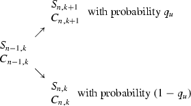
To extend the binomial model to several periods, in an effort to develop a model for option pricing and hedging which includes the possibility of dynamic portfolio allocation, we consider a total number of periods $N\ge 2$, and iterate the one-period construction of the previous section, over several periods, forming what is known as a binomal tree, with the root typically represented at the left, and the leaves at the right, i.e. with time running from left to right. For $N=2$, this tree representation for the two-period binomial model has the following form

Note that the tree has the so-called “recombining” property, because the up and down factors do not change. More generally, for $N\ge 2$, and $n=1{,}2{,}\ldots {,}N$, $k=0{,}1,2{,}\ldots {,}\,n$, period number n models the dynamics during the time interval $[n-1{,}\,n]$, and the node $(n{,}\,k)$ is the name of the position in the tree at time n for any stock price path which takes k up steps and $n-k$ down steps, from time 0 to time n. This parametrization of nodes is only possible because of the recombining property. This property works because the up and down factors u, d do not depend on the position in the tree at a fixed time (u and d might depend on time n, this does not impact the recombining property). In particular, the value of S at node $\left( n{,}k\right)$ is

$$\begin{aligned} S_{n{,}k}:=S_{0}u^{k}d^{n-k}. \end{aligned}$$

Again in the case where u and d depend only on n (we will not consider other cases in these notes), let us translate the binomial model in a more probabilist fashion. Let $q_{u}$ be probability to go up at every node. Assume $q_{u}$ is constant. For every $n=1{,}\ldots {,}N$, we can consider the random variable $K_{n}$ representing the number of times that the stock went up rather than down between time 0 and time n. Then $K_{n}= \sum _{i=1}^{n}\varepsilon _{i}$ where $\varepsilon _{i}=1$ if the stock went up in the interval $[i-1{,}1]$, and $\varepsilon _{i}=0$ if the stock went down. Each $\varepsilon _{i}$ is a Bernoulli random variable with parameter $q_{u}$. Assuming all the $\varepsilon _{i}$’s are independent, $K_{n}$ is thus a binomial random variable with parameters $n{,}q_{u}$. This is from whence the binomial model gets its name. The stock price model then has the following probabilistic representation: for $n=0{,}\ldots {,}N$,

$$\begin{aligned} S_{n}=S_{0}u^{K_{n}}d^{n-K_{n}}=S_{0}e^{\left( \ln d\right) n+\ln \left( u/d\right) K_{n}}. \end{aligned}$$

4 Option Pricing and Hedging Algorithm: Backwards Recursion

Assume we need to price and hedge a simple European claim with contract function $\varPhi$. We may use the pricing and hedging scheme from the one-period model iteratively backwards in time to price and hedge options in the N-period binomial model.

• At time N, value of option = value of payoff = $C_{N}=\varPhi (S_{N})$

  In node notation, if number of up steps $=k$ then $S_{N}=S_{0}u^{k}d^{N-k}$. Thus:

  Initialization:

  $C_{N{,}k}=\varPhi (S_{0}u^{k}d^{N-k})$ for all $k=0{,}1{,}\ldots {,}N$.

   

• To implement the recursion, assume that at some time $n\le N$ ; $C_{n{,}k}$ is known for every $k=0{,}1{,}\ldots {,}\,n$. Then, for each $k=0{,}1{,}\ldots {,}\,n-1$, by using the formula for pricing in the one-period binomial model which goes from node $\left( n-1{,}\,k\right)$ to the two possible future nodes $\left( n{,}\,k\right)$ and $\left( n{,}\,k+1\right)$, i.e. the tree, in which each node contains stock and option prices,

  

  we obtain the following price recursion:

  Recursion: option prices:

  $C_{n-1{,}k}=e^{-rh}\left( q_{u}C_{n{,}k}+(1-q_{u})C_{n{,}k-1}\right)$ for each $n=1{,}\ldots {,}N$ and $k=0{,}1{,}\ldots {,}\,n-1$.

   

• We must also compute the hedging portfolio at node $(n-1{,}\,k)$: this can either be computed while implementing the previous recursion, or offline after all option prices are known. By the one-period hedging portfolio, this is

  Hedge: number of shares of stock:

  $$\begin{aligned} y_{n-1{,}k}=\frac{C_{n{,}k+1}-C_{n{,}k}}{S_{n{,}k+1}-S_{n{,}k}}=\frac{C_{n{,}k+1}-C_{n{,}k} }{S_{n-1{,}k}(u-d)}. \end{aligned}$$

  Hedge: wealth in risk-free account:

  $$\begin{aligned} b_{n-1{,}k}=C_{n-1{,}k}-S_{n-1{,}k}y_{n-1{,}k}. \end{aligned}$$

• The above scheme provides a perfect hedge which can be followed dynamically in time, and reacts to the changes in stock prices over each period. Indeed, at time $n-1$, the hedging decision only requires knowledge of the observed stock price $S_{n-1}=S_{n-1{,}K_{n-1}}$ (under the binomial model, the random variables $S_{n-1}$ and $K_{n-1}$ can be computed one from the other; they share the same information), and of the two possible future values for $C_{n}$, which are $C_{n{,}K_{n-1}+1}$ and $C_{n{,}K_{n-1}}$ which are among the precomputed values in the binomial tree.

• As an option hedger (also known as an option market maker), one must consider the trade-off between assuming that the length of the time in one’s binomial model is short enough to stick closely to the stock variations, and incurring many transaction costs every time one rebalances one’s hedging portfolio. In practice, stock prices change many more times than once a day. Yet market makers often assume that $h=1/365=1$ day nonetheless. When we enter our discussion of continuous-time modeling with discrete-time hedging, we will provide a way to compute the discrepancy between a perfect hedge and the need to keep the hedging frequency down to a reasonable, daily level.

• Recall probabilistic representation of the option price for one period: price at time 0 $=e^{-rh}\mathbf {E}^{\mathbf {Q}}\left[ \mathscr {X} _{h}\right] .$ Such a formula also holds for the multiperiod model, and it is easy to prove this by using the one-period formula and the recursion formula for the multi-period model given here. The details are left to the reader.

  Discounted Risk Neutral Valuation Formula: multi-period case:

  With maturity $T=Nh$, define the contingent claim $\mathscr {X}_{T}=\varPhi \left( S\left( T\right) \right)$, the risk-neutral (martingale) measure $\mathbf {Q}$ is defined by using the risk-neutral probabilities $q_{u}$ and $1-q_{u}$ in each period. Then we have

  $$\begin{aligned} \text {price of }\mathscr {X}_{T}\text { at time }0=e^{-rT}\mathbf {E}^{\mathbf {Q }}\left[ \mathscr {X}_{T}\right] . \end{aligned}$$

4.1 How to Estimate/Calibrate Parameters r, u and d?

We provide some brief recommendations for the parameter estimation question.

An excellent proxy for the rate r is the LIBOR (London Interbank Offered Rate) short (overnight) rate L: this is the average rate at which banks lend each other money over a 24-hour period. This is thus most appropriate when $h=1/365$, and one sets $e^{rh}=1+L$. Since the LIBOR short rate changes over time, one typically uses the previous day’s value of L to calibrate r. There exist stochastic models of interest rates that take into account the uncertainty on future values of L. They are not discussed in these notes.

For u and d, it is typical to base their estimation/calibration using the concept of “historical volatility”, which can be defined, for instance, as the empirical standard deviation, over an appropriately long time period, of $h^{-1/2}\mathscr {R}_{t}$ where $\mathscr {R}_{t}$ are the log returns $\mathscr {R}_{t}:=\log \left( S\left( t-h\right) /S\left( t\right) \right)$ where $\left( S\left( t\right) \right) _{t}$ are the past stock price data, which can thus be identified, insofar as it represents a consistent estimator, with the square root $\sigma$ of

$$\begin{aligned} \sigma ^{2}:=Var\left( \mathscr {R}_{t}\right) \end{aligned}$$

where now the notation $\mathscr {R}_{t}$ comes from a specific model, as long as this variance does not depend on t (stationarity).

There are many other ways of determining volatility models, some of which involve assuming that volatility is random itself. An emerging method for determining volatility is becoming popular in the case of the S&P 500 index. Since 1993, the Chicago Board of Options Exchange (CBOE) has published a composite value of option prices on this equity index, which can be interpreted as a 30-day average of volatility on the index. This volatility index, now known as the VIX, increased in popularity since the CBOE started offering traded options and futures contracts on the VIX starting in 2004.

Once a value of $\sigma$ has been determined, a common method for calibrating u and d using the so-called Cox-Ross-Rubenstein parametrization:

$$\begin{aligned} u= & {} e^{\sigma \sqrt{h}}, \\ d= & {} e^{-\sigma \sqrt{h}}. \end{aligned}$$

Other choices include the Hull-White parametrization $u=1+\alpha h+\sigma \sqrt{h}$, $d=1+\alpha h-\sigma \sqrt{h}$; as well as the Jarrow-Rudd parametrization $u=e^{\mu h+\sigma \sqrt{h}}$, $d=e^{\mu h-\sigma \sqrt{h}}$, where the values of $\alpha$ and $\mu$ are $h^{-1}$ times the expected values of the log returns $\mathscr {R}_{t}$ or the simple returns $R_{t}=\left( S\left( t+h\right) -S\left( t\right) \right) /S\left( t\right)$.

Understanding the differences between these various parametrizations can be done in conjunction with the introduction of the continuous-time analogue to the Binomial model, the so called Black-Scholes model, where the volatility parameter $\sigma$ plays a rather clear role, as we now discuss.

5 Black-Scholes Model (Single Stock)

The classical Black-Scholes model with constant coefficients contains the following two elements, for any $t\in [0{,}T]$ where T is a maturity or time horizon:

• A risk-free account B with constant rate r:

  $$\begin{aligned} B(t)=e^{rt}. \end{aligned}$$

• A stock or index price process S:

  $$\begin{aligned} S(t)=S(0)e^{(\alpha -\frac{1}{2}\sigma ^{2})t+\sigma W(t)}. \end{aligned}$$

  Here, we use the nomenclature $\alpha =$ “mean rate of return” for stock S, and $\sigma =$ “volatility” for stock S; while $\{W(t);t\ge 0\}$ is a standard Brownian motion (Wiener process).

  The process W has the following properties:

  • $W\left( 0\right) =0$, for $0\le s<t$, $W\left( t\right) -W\left( s\right)$ is independent of all the random variables $W\left( r\right)$ for $r\le s$, and $W\left( t\right) -W\left( s\right)$ is centered normal with variance $t-s$.

  • W has continuous paths with probability one.

• Convenient notation: $\mu :=\alpha -\frac{1}{2}\sigma ^{2}$.

• These parameters $\alpha ,\sigma ,\mu$ are assimilated to quantities similarly to those in the discussion at the end of the previous section: specifically it holds that

$$\begin{aligned} \alpha= & {} \lim _{h\downarrow 0}E[\frac{S(t+h)-S(t)}{h}] \\ \mu= & {} \lim _{h\downarrow 0}E[\frac{1}{h}\log (\frac{S(t+h)}{S(t)})] \\ \sigma ^{2}= & {} \lim _{h\downarrow 0}Var[\frac{S(t+h)-S(t)}{h}] \\= & {} \lim _{h\downarrow 0}Var[\frac{1}{h}\log (\frac{S(t+h)}{S(t)})]. \end{aligned}$$

Example 1

Today is time $t=T=Nh$; let $\ S_{i}=S(ih)$; $i=0{,}1{,}\ldots {,}N$. Then $\sigma ^{2}$ can be estimated as the rescaled empirical variance of the sequence of log returns:

$$\begin{aligned} \sigma ^{2}\approx \hat{\sigma }^{2}: & {} =\frac{1}{N}\sum _{i=0}^{N-1}\left( \frac{1}{\sqrt{h}}\log \left( \frac{S_{i+1}}{S_{i}}\right) -\frac{1}{\sqrt{h} }E\left[ \log \left( \frac{S_{i+1}}{S_{i}}\right) \right] \right) ^{2} \\= & {} \frac{1}{h}\frac{1}{N}\sum _{i=0}^{N-1}\left( \log \left( \frac{S_{i+1}}{ S_{i}}\right) -\mu h\right) ^{2}, \end{aligned}$$

since $Var\left[ \log \left( \frac{S_{i+1}}{S_{i}}\right) \right] =Var\left[ \sigma W\left( \left( i+1\right) h\right) -\sigma W\left( ih\right) \right] =\sigma ^{2}h$. Using same idea, we can also get estimators for $\mu$ and $\alpha .$

5.1 Method of Moments

To explain the parameter choices made at the end of the previous section, one only needs to match the means and variances (first and second moments) of the stock returns over one period in the binomial model, to the same statistics in the Black-Scholes model in a period of length h, by using various specific choices for the objective probabilities of going up or down:

• We compute the log and simple returns in the Black-Scholes model:

  $$\begin{aligned} \mathscr {R}_{t}= & {} \log (\frac{S(t+h)}{S(t)})=\mu h+\sigma (W(h+t)-W(t)), \\ R_{t}= & {} \frac{S\left( t+h\right) -S\left( t\right) }{St}=e^{\mu h+\sigma (W(h+t)-W(t))}-1, \end{aligned}$$

  so that we compute can compute their means and variances, and their asymptotics for small h:

  $$\begin{aligned} \mathbf {E}\left[ \mathscr {R}_{t}\right]= & {} \mu h, \\ Var\left[ \mathscr {R}_{t}\right]= & {} \sigma ^{2}h, \\ \mathbf {E}\left[ R_{t}\right]= & {} e^{\alpha h}-1\approx \alpha h, \\ Var\left[ R_{t}\right]= & {} e^{\left( 2\mu +\sigma ^{2}\right) h}\left( e^{\sigma ^{2}h}-1\right) \approx \sigma ^{2}h. \end{aligned}$$

• One possibility is to look for the binomial model with equal probabilities $p_{u}=1-p_{u}=0.5$ of going up or down, and matching its simple returns’ expectation and variance. Since then $R_{t}=\left( S_{1}-S_{0}\right) /S_{0}=u-1$ or $d-1$ with probabilities 0.5 and 0.5, those binomial statistics are

  $$\begin{aligned} \mathbf {E}\left[ R_{t}\right]= & {} \frac{u+d}{2}-1, \\ Var\left[ R_{t}\right]= & {} \frac{1}{2}\left( \left( u-1\right) ^{2}+\left( d-1\right) ^{2}\right) -\left( \frac{u+d}{2}-1\right) ^{2} \\= & {} \left( \frac{u-d}{2}\right) ^{2}. \end{aligned}$$

  In the case of small h, this yields (approximately) the system

  $$\begin{aligned} \left\{ \begin{array}{c} \alpha h+1=\frac{u+d}{2} \\ \sigma \sqrt{h}=\frac{u-d}{2} \end{array} \right. \end{aligned}$$

  whose solution is easily seen to be

  $$\begin{aligned} u=1+\alpha h+\sigma \sqrt{h}{,}d=1+\alpha h-\sigma \sqrt{h} \end{aligned}$$
  $$\begin{aligned} p_{u}=\frac{1}{2}. \end{aligned}$$

  We recognize the Hull-White parametrization.

• Another possibility is to decide that one prefers to have up and down factors which are reciprocals of each other. By inspecting the Black-Scholes model, ignoring the drift term $\mu t$ and concentrating only on the term $\sigma W_{t}$ inside the exponential, one knows that an order of magnitude of the change of $\sigma W_{t}$ over a period of length h is its standard deviation, namely $\sigma \sqrt{h}$. It is then legitimate to require that $u=\frac{1}{d}=\exp (\sigma \sqrt{h}).$ However, let us use the method of moments using only the restriction $u=1/d$. We can compute mean and variance of the log return $\mathscr {R}_{t}$ in the one peroid binomial, finding

  $$\begin{aligned} \mathbf {E}\left[ \mathscr {R}_{t}\right]= & {} p_{u}\log u+\left( 1-p_{u}\right) \log u^{-1} \\= & {} \left( 2p_{u}-1\right) \log u \\ Var\left[ \mathscr {R}_{t}\right]= & {} p_{u}\log ^{2}u+\left( 1-p_{u}\right) ^{2}\log ^{2}u-\left( 2p_{u}-1\right) ^{2}\log ^{2}u \\= & {} \left( 1-\left( 2p_{u-1}\right) ^{2}\right) \log ^{2}u. \end{aligned}$$

  Using the approximation that if h is small, p should be close to 1 / 2, matching the above variance with the Black-Scholes variance yields $\log ^{2}u=\sigma ^{2}h$, which is precisely

  $$\begin{aligned} u=\frac{1}{d}=e^{\sigma \sqrt{h}}. \end{aligned}$$

  Plugging this into the equation for matching expectations $\left( 2p_{u}-1\right) \log u=\mu h$, we get, $\sigma \sqrt{h}\left( 2p_{u}-1\right) =\mu h$, i.e.

  $$\begin{aligned} p_{u}=\frac{1}{2}+\frac{\mu }{2\sigma }\sqrt{h}. \end{aligned}$$

  This is the Cox-Ross-Rubenstein parametrization.

• One last possibility we examine is the case of matching means and variances of the log returns when $p_{u}=1/2$. In this case, we compute those statistics for the Binomial model

  $$\begin{aligned} \mathbf {E}\left[ \mathscr {R}_{t}\right]= & {} \frac{1}{2}\left( \log u+\log d\right) \\ Var\left[ \mathscr {R}_{t}\right]= & {} \frac{1}{2}\left( \log ^{2}u+\log ^{2}d\right) -\frac{1}{4}\left( \log u+\log d\right) ^{2} \\= & {} \left( \frac{\log u-\log d}{2}\right) ^{2}. \end{aligned}$$

  In this case, the moment-matching equations can be solved without resorting to approximations, and one finds

  $$\begin{aligned} u= & {} e^{\mu h+\sigma \sqrt{h}}, \\ d= & {} e^{\mu h-\sigma \sqrt{h}}, \\ p_{u}= & {} \frac{1}{2}. \end{aligned}$$

  This is the Jarrow-Rudd parametrization. This parametrization is closest in spirit to the original Black-Scholes model, if one attempts to discretize it in time by replacing each Brownian increment $W_{t+h}-W_{t}$ by a random variable taking the values $+\sigma \sqrt{h}$ and $-\sigma \sqrt{ h}$ with equal probabilities, owing to the standard deviation and symmetry of the normal law for this increment. In fact, the binomal model with Jarrow-Rudd parameters converges to the Black-Scholes model. The proof of this fact is nearly immediate for fixed t by using the central limit theorem; that the convergence also holds at the process level (i.e. for all t simultaneously) is an application of the infinite-dimensional (functional) extension of the central limit theorem, sometimes known as Donsker’s invariance principle.

The fact that there are several parametrization choices show that the binomal model is in fact richer than the Black-Scholes model; the former has one more parameter than the latter, hence the existence of many parametrization choices.

5.2 Option Pricing Under BS Model

Because of the close similarity between the binomial model with Jarrow-Rudd parameters and the Black-Scholes model, one suspects that the discounted risk-neutral valuation formula should hold for the Black-Scholes model. This is in fact true, and there is a generic option-pricing meta-theorem, which is broader than merely the Black-Scholes model, and also includes a statement about hedging.

 

Pricing metatheorem:

Let S be a stock price model, and let $\mathscr { X}$ be a contingent claim expiring at time T, i.e. $\mathscr {X}$ is a random variable which can be determined at time T using knowledge of the path of the stock price S up to time T. If the model for S can be expressed with a probability measure $\mathbf {Q}$ under which $t\rightarrow e^{-rt}S\left( t\right)$ is a martingale with respect S, then all contingent claims can be simultaneously priced in a consistent way via the formula

$$\begin{aligned} \text {price of }\mathscr {X}_{T}\text { at time }0=e^{-rT}\mathbf {E}^{\mathbf {Q }}\left[ \mathscr {X}_{T}\right] . \end{aligned}$$

If the measure $\mathbf {Q}$ is unique, then the price of every contingent claim is unique, and each such claim can be perfectly hedged (in continuous time) using a continuously-rebalanced self-financing portfolio of stock S and risk-free asset B.

In the case of Markovian models such as the Black-Scholes model, much more can be said about simple claims. We state the result in the Black-Scholes case only, for simplicity.

Definition 1

We say that $\mathscr {X}$ is a simple “contingent claim” (= a simple “option”) if there as a non-random function $\varPhi :\mathbb {R}_{+}$ $\rightarrow \mathbb {R}$ such that $\mathscr {X}=\varPhi (S(T))$ (here T = maturity).

Theorem 1

(Discounted Risk-Neutral Valuation Formula) Assume S satisfies the Black-Scholes model. The price $P_{t}$ at time $t\le T$ for the claim $\mathscr {X}$ defined above, is given by

$$\begin{aligned} P_{t}=F(t{,}S(t)) \end{aligned}$$

where the non-random function $F:\left[ 0{,}T\right] \times \mathbb {R}_{+}$ $\rightarrow \mathbb {R}$ is given by

$$\begin{aligned} F(t{,}x)=\exp (-r(T-t))\mathbf {E}^{*}\left[ \varPhi (S(T))/S(t)=x\right] , \end{aligned}$$

where $\mathbf {E}^{*}$ is the expectation under $\mathbf {P}^{*}$ the unique risk-neutral (martingale) measure. Moreover, $\mathbf {P}^{*}$ can be defined by saying that under $\mathbf {P}^{*}$, the parameter $\alpha$ in the Black-Scholes model need only be replaced by the risk-free rate r.

5.3 Black-Scholes Formula

We may now use the meta-theorem’s application to the Black-Scholes model, which we have just stated, to calculate the price of call options.

Definition 2

Let K be a positive constant. A simple contingent claim with contract function given by $\varPhi (x)=\max (x-K{,}0)$, is a Call option with strike price K.

We wish to compute F(t, x) in the previous theorem when $\varPhi (x)=\max (x-K{,}0)$ and $S(t)=$ Black-Scholes model under $\mathbf {P}^{*}$. This can be done to a large extent by hand:

$$\begin{aligned} F(t{,}x)= & {} \exp (-r(T-t))\mathbf {E}^{*}\left[ \max (x-K{,}0)/S(t)=x\right] \\= & {} \exp (-r(T-t))\mathbf {E}[\max (x\exp (\mu ^{*}(T-t)+\sigma (W(T)-W(t)))-K{,}0)] \\= & {} \exp (-r(T-t))\mathbf {E}[\max (x\exp (\mu ^{*}(T-t)+\sigma \sqrt{T-t} Z)-K{,}0)] \end{aligned}$$

where in the second line, we denote

$$\begin{aligned} \mu ^{*}:=r-\sigma ^{2}/2 \end{aligned}$$

(i.e. we use the parameters for S under $\mathbf {P}^{*}$), and in the last line, thanks to scaling for normal laws, we assume that Z is a standard normal random variable. Note that, starting with the second displayed line above, it becomes unnecessary to add a star to the expectation sign. We also see that the last expression above depends on T and t only via $T-t$. Hence without loss of generality we set $t=0$. Thus

$$\begin{aligned} F\left( 0{,}x\right)= & {} e^{-rT}\mathbf {E}\left[ \max (x\exp (\mu ^{*}T+\sigma \sqrt{T}Z)-K{,}0)\right] \\= & {} e^{-rT}\mathbf {E}\left[ [\mathbf {1}_{\{x\exp (\mu ^{*}T+\sigma \sqrt{T }Z)>K\}}(x\exp (\mu ^{*}T+\sigma \sqrt{T}Z)-K)\right] \\= & {} xe^{-rT}\mathbf {E}\left[ \mathbf {1}_{\{x\exp (\mu ^{*}T+\sigma \sqrt{T }Z)>K\}}\exp (\mu ^{*}T+\sigma \sqrt{T}Z)\right] \\&-Ke^{-rT}\mathbf {P} \left[ x\exp (\mu ^{*}T+\sigma \sqrt{T}Z)>K\right] . \end{aligned}$$

We first compute the second piece:

$$\begin{aligned} P\left[ x\exp (\mu ^{*}T+\sigma \sqrt{T}Z)>K\right]= & {} P\left[ Z>\frac{1 }{\sigma \sqrt{T}}\left( -\mu ^{*}T+\log \left( \frac{K}{x}\right) \right) \right] \\= & {} P\left[ Z<\frac{1}{\sigma \sqrt{T}}\left( \mu ^{*}T+\log \left( \frac{ x}{K}\right) \right) \right] \\: & {} =P\left[ Z<d_{2}\right] \\: & {} =N(d_{2}) \end{aligned}$$

where N is the cummulative distribution function of the standard normal $N\left( d\right) =\left( 2\pi \right) ^{-1/2}\int _{-\infty }^{d}e^{-z^{2}/2}dz$ and

$$\begin{aligned} d_{2}:=\frac{1}{\sigma \sqrt{T}}\left( \mu ^{*}T+\log \left( \frac{x}{K} \right) \right) =\frac{1}{\sigma \sqrt{T}}\left( \left( r-\sigma ^{2}/2\right) T+\log \left( \frac{x}{K}\right) \right) . \end{aligned}$$

For the first piece, the computation is not much harder:

$$\begin{aligned}&xe^{-rT}\mathbf {E}\left[ \mathbf {1}_{\{x\exp (\mu ^{*}T+\sigma \sqrt{T} Z)>K\}}\exp (\mu ^{*}T+\sigma \sqrt{T}Z)\right] \\= & {} xE\left[ \exp \left( - \frac{1}{2}\sigma ^{2}T+\sigma \sqrt{T}Z\right) \mathbf {1}_{\{Z>-d_{2}\}} \right] \\= & {} xE\left[ \exp \left( -\frac{1}{2}\sigma ^{2}T-\sigma \sqrt{T}\left( -Z\right) \right) \mathbf {1}_{\{-Z<d_{2}\}}\right] \\= & {} xe^{-rT}\int _{-\infty }^{d_{2}}\exp \left( -\frac{1}{2}\sigma ^{2}T-\sigma \sqrt{T}z\right) \exp (-\frac{z^{2}}{2})\frac{dz}{^{\sqrt{2\pi } }} \\= & {} x\int _{-\infty }^{d_{2}}\exp \left( -\frac{1}{2}(z+\sigma \sqrt{T} )^{2}\right) \frac{dz}{^{\sqrt{2\pi }}} \\= & {} x\int _{-\infty }^{d_{2}+\sigma \sqrt{T}}\exp \left( -\frac{z^{2}}{2} \right) \frac{dz}{^{\sqrt{2\pi }}} \\= & {} xN(d_{2}+\sigma \sqrt{T}) \\:= & {} xN(d_{1}) \end{aligned}$$

where

$$\begin{aligned} d_{1}:=\frac{1}{\sigma \sqrt{T}}\left( \left( r+\sigma ^{2}/2\right) T+\log \left( \frac{x}{K}\right) \right) . \end{aligned}$$

We proved the famous Black-Scholes formula for pricing.

Theorem 2

The pricing function F of the call option with strike K under the standard Black-Scholes model is:

$$\begin{aligned} F(t{,}x)=xN(d_{1})-Ke^{-r(T-t)}N(d_{2}) \end{aligned}$$

where N is the standard normal distribution function and

$$\begin{aligned} d_{1}: & {} =\frac{1}{\sigma \sqrt{T-t}}(\log (\frac{x}{K})+(r+\frac{1}{2} \sigma ^{2})(T-t)), \\ d_{2}: & {} =\frac{1}{\sigma \sqrt{T-t}}(\log (\frac{x}{K})+\left( r-\frac{1}{2} \sigma ^{2}\right) (T-t)) \\= & {} d_{1}-\sigma \sqrt{T-t}. \end{aligned}$$

Remark 1

This formula has an interesting feature, which is to suggest a possible way of hedging the option over time: indeed, if at time t, where the stock price is $S\left( t\right)$, one invests in $N\left( d_{1}\right)$ shares of stock (here x must be replaced by the current stock value $S\left( t\right)$ in the formulas), then by also holding

$$\begin{aligned} F(t{,}S(t))-S(t)N(d_{1})=-Ke^{-r(T-t)}N(d_{2}) \end{aligned}$$

dollars in the risk-free asset, one obtains a replicating portfolio for the option, i.e. one whose value is exactly that of the option at all times. This will be a worthwhile observation if one can prove that the portfolio is self-financing.

Remark 2

As it turns out, the previous portfolio really is self-financing, meaning that all changes in the portfolio allocations can be financed by the changes in the asset prices. We record this fact formally here, but rather enter into a formal proof, in the next section, we investigate how far from a perfect hedge one might get when the hedging portfolio is followed appriximately, by using discrete time.

Theorem 3

(Perfect Black-Scholes Hedge) The Call option with strike-price K and maturity T can be perfectly replicated using the following portfolio: $y_{t}$ shares of stock S and $b_{t}$ dollars in the risk-free asset, with

$$\begin{aligned} y_{t}= & {} N(d_{1}), \\ b_{t}= & {} -Ke^{-r(T-t)}N(d_{2}) \end{aligned}$$

where x is replaced by $S\left( t\right)$ in the formulas for $d_{1}$ and $d_{2}$. This portfolio is self-financing.

More generally, for the pricing function F of a given contingent claim $\mathscr {X}=\varPhi \left( S\left( T\right) \right)$, under the Black-Scholes model, the hedging portfolio defined by

$$\begin{aligned} y_{t}:=\frac{\partial F}{\partial x}\left( t{,}S(t)\right) ;\;\;\;b_{t}:=F\left( t{,}S\left( t\right) \right) -S\left( t\right) y_{t} \end{aligned}$$

is replicating by definition, and is self-financing.

6 Imperfect Black-Scholes Hedging in Discrete Time

6.1 Overnight Rebalancing, with Profit (Loss) Calculation

We mentioned earlier that following a trading strategy in continuous time is not practical. The replicating strategy $(y_{t\text { }}{,}b_{t})$ in the previous theorem is not immune to this difficulty. In practice, a high-frequency trading strategy (e.g. rebalancing every 5 min) can take advantage of rapid changs in stock values, but is too expensive to implement because of transaction costs.

Question: What happens if we follow the Black-Scholes hedging strategy only once a day?

We will use the arguments $\left( t{,}x\right)$ and $\left( t+h{,}x+\varepsilon \right)$ for expressions F, $d_{1}$ and $d_{2}$, as shorthand notation, with the following understanding:

$$\begin{aligned} t= & {} \text {today} \\ h= & {} 1/365 \\ t+h= & {} \text {tomorrow} \\ x= & {} S\left( t\right) =\text {price of stock today} \\ x+\varepsilon= & {} S\left( t+h\right) =\text {price of stock tomorrow.} \end{aligned}$$

Taking the perspective of the option hedger, we sell one option at time t and purchase its corresponding Black-Scholes perfect hedging portfolio at the same time, and hold that portfolio without any rebalancing until time $t+h$. The value of the portfolio at time t is 0 by the hedging theorem. Let us investigate the so-called “overnight profit (or loss)”; this is thus identical to the value of the portfolio at time $t+h$ before rebalancing:

• Value held in option: $-F\left( t+h{,}x+\varepsilon \right) .$

• Value held in stock: $\left( x+\varepsilon \right) N\left( d_{1}\left( t{,}x\right) \right) .$

• Value held in risk-free asset: $\left( F(t{,}x)-xN(d_{1})\right) e^{rh}.$

• Total value held is: Overnight profit (or loss)

  $$\begin{aligned} =-F(t+h{,}x+\varepsilon )+(x+\varepsilon )N(d_{1}(t{,}x))+\left( F(t{,}x)-xN(d_{1}\left( t{,}x\right) )\right) e^{rh}. \end{aligned}$$

Example 2

In our numerical applications, we use: $x=40$; $\varepsilon =0.5$; $\sigma =0.3$; $r=0.08$; $h=1/365$; we choose to price the call with $K=40$ and $T-t=1/4$ (3 months).

By using BS formula we find $F(t{,}x)=2{,}7847$ ; $N(d_{1}(t{,}x))=0{,}5825$ ; $F(t{,}x)-xN(d_{1})=-20{,}5159$ ; $F(t+h{,}x+\varepsilon )=3{,}0665$. Thus in this case:

$$\begin{aligned} \mathbf {Option\,hedger}\text {'}\mathbf {s\,overnight\,profit}= & {} -3{,}0665+0{,}5824\times 40{,}5-20{,}5159e^{0.08/365}, \\= & {} 0{,}00500. \end{aligned}$$

This is great: this is very close to 0, so there is probably no need to buy or sell stock to rebalance the portfolio at time $t+h$.

Example 3

However, the good news in the previous example is due to the fact that the stock price did not move very far (only about $1\,\%$) overnight. One might run into more trouble if the movements are larger. Repeating the previous calculations for various values of $\varepsilon$, we obtain the following Figures.

Fig. 1

Overnight profit for values of $x+\varepsilon$ from 35 to 45. Vertical axis is dollar value

Fig. 2

Detail of overnight profit for values of $x+\varepsilon$ from 39 to 41

Figure 1 shows that when large stock price movements occur, the overnight profit quickly becomes a substantial loss. Figure 2 shows in detail the small magnitude of profit or loss when stock price changes are small (for $S\left( t+h\right)$ near $S\left( t\right)$.) An actual small profit occurs for $\left| S\left( t+h\right) -S\left( t\right) \right| <0.6$ only.

We finish this section by mentioning the general form of the overnight profit under the Black-Scholes model.

Theorem 4

(Overnight profit for general simple claims under the Black-Scholes model) With the pricing function F of a given contingent claim $\mathscr {X}=\varPhi \left( S\left( T\right) \right)$, under the Black-Scholes model, by following the hedging portfolio defined by $y_{t}:= \frac{\partial F}{\partial x}\left( t{,}S(t)\right) ;\;b_{t}:=F\left( t{,}S\left( t\right) \right) -S\left( t\right) y_{t}$ at discrete time intervals of length h, the overnight profit at time t is

$$\begin{aligned} -F(t+h{,}x+\varepsilon )+(x+\varepsilon )\frac{\partial F}{\partial x}\left( t{,}x\right) +\left( F(t{,}x)-x\frac{\partial F}{\partial x}\left( t{,}x\right) \right) e^{rh}. \end{aligned}$$

6.2 Forecasting

To understand the previous graph in theory, instead of analyzing the Black-Scholes formula in a mechanistic way (i.e. looking only at its dependence on t and x as a deterministic function), one may return to the probabilistic understanding and employ some simple forecasting. A rough approximation is in fact sufficient. Under the Black-Scholes model we can compute

$$\begin{aligned} S(t+h)-S\left( t\right)= & {} S\left( t\right) \exp \left( \mu h+\sigma (W(t+h)-W(t))\right) -S\left( t\right) \\= & {} S\left( t\right) \left( \exp \left( \mu h+\sigma (W(t+h)-W(t))\right) -1\right) . \end{aligned}$$

Since h is considered small, and the typical size of the mean-zero increment $W(t+h)-W(t)$ is the size of its standard deviation, i.e. $\sqrt{h}$, one may consider in a first approximation that $W(t+h)-W(t)$ is small and dominates $\mu h$. Thus, using the first order Taylor expansion of the exponential function, we would get

$$\begin{aligned} S(t+h)-S(t)=S\left( t\right) \left( \sigma (W(t+h)-W(t))\right) +o(\sqrt{h}). \end{aligned}$$

We may interpret this approximation in a binary way, as

$$\begin{aligned} S(t+h)-S(t)\simeq (\pm 1)\sigma \sqrt{h}S(t). \end{aligned}$$

In other words, with the x and $\varepsilon$ notation, this approximation is equivalent to:

$$\begin{aligned} \varepsilon \simeq (\pm 1)\sigma \sqrt{h}{x} \end{aligned}$$

where the $(\pm 1)$ symbol represents a random variable which takes values $+1$ and $-1$ with equal probabilities.

Using Taylor’s formula on F up to order 1 in time and order 2 in space, we obtain

$$\begin{aligned} F(t+h{,}x+\varepsilon )=F(t{,}x)+h\frac{\partial F}{\partial t}(t{,}x)+\varepsilon \frac{\partial F}{\partial x}(t{,}x)+\frac{1}{2}\varepsilon ^{2}\frac{\partial ^{2}F}{\partial x^{2}}(t{,}x)+o(h)+o(\varepsilon ^{2}). \end{aligned}$$

Therefore,

$$\begin{aligned} \text {overnight profit}= & {} -\left[ F(t{,}x)+h\frac{\partial F}{\partial t} (t{,}x)+\varepsilon \frac{\partial F}{\partial x}(t{,}x)+\frac{1}{2}\varepsilon ^{2}\frac{\partial ^{2}F}{\partial x^{2}}(t{,}x)\right] \\&+\frac{\partial F}{\partial x}\left( t{,}x\right) (x+\varepsilon )+\left[ F(t{,}x)-x\frac{\partial F}{\partial x}\left( t{,}x\right) \right] (1+rh)+o(h)+o(\varepsilon ^{2}). \end{aligned}$$

One notes that all the terms involving $\varepsilon$ rather $\varepsilon ^{2}$ miraculously disappear, as do all the terms which are not small: this is because the Black-Scholes hedge was chosen in such a way to make these simplications occur, at least in the first approximation we are using here. Thus we get overnight profit

$$\begin{aligned} =-h\frac{\partial F}{\partial t}(t{,}x)-\frac{1}{2} \varepsilon ^{2}\frac{\partial ^{2}F}{\partial x^{2}}(t{,}x)+rhx\frac{\partial F}{\partial x}\left( t{,}x\right) +rhF(t{,}x)+o(h)+o(\varepsilon ^{2}). \end{aligned}$$

Interestingly, in a first-order approximation on $\varepsilon$, one sees that if $\frac{\partial ^{2}F}{\partial x^{2}}(t{,}x)>0$, which is typically the case for most options, the highest overnight profit is obtained when $\varepsilon$ is 0. Now using the forecast for $\varepsilon$, we see that $\varepsilon ^{2}=\sigma ^{2}h$ and that $o(h)=o(\varepsilon ^{2})$. This yields

$$\begin{aligned} \text {overnight profit}=\left( rF(t{,}x)-\frac{\partial F}{\partial t}(t{,}x)- \frac{1}{2}\sigma ^{2}x^{2}\frac{\partial ^{2}F}{\partial x^{2}}(t{,}x)-rx \frac{\partial F}{\partial x}(t{,}x)\right) h+o\left( h\right) . \end{aligned}$$

The option hedger must try to keep her profit to a minimum in absolute value, as one should from the perspective of an insurer, which is to minimize risk (it is also a good idea from an investment perspective, since we saw in the previous section that the overnight profit’s downside is significantly greater than its upside.) This risk-minimizing strategy can thus be summarized as “Overnight profit $=0$”

$$\begin{aligned} \iff \text { }\frac{\partial F}{\partial t}\left( t{,}x\right) +rx\frac{\partial F}{ \partial x}\left( t{,}x\right) +\frac{1}{2}\sigma ^{2}x^{2}\frac{\partial ^{2}F }{\partial x^{2}}\left( t{,}x\right) -rF\left( t{,}x\right) \!=\!0. \end{aligned}$$

This is precisely the famous so-called BLACK-SCHOLES PDE !

What we have essentially just shown is that the Black-Scholes hedge is a perfect self-financing replicating portfolio if and only if the Black-Scholes PDE holds for the pricing function F. In fact, the above development is in some sense equivalent to the classical proof of the Black-Scholes pricing and hedging theorem by means of stochastic calculus and the Itô formula. We do not provide the details, but state the result formally, also summarizing our theorems on the discounted risk-neutral valuation formula and the perfect Black-Scholes hedge.

Theorem 5

For a generic simple European contingent claim $\mathscr {X}=\varPhi (S(T))$ under the Black-Scholes model, let

$$\begin{aligned} F\left( t{,}x\right) =e^{-r\left( T-t\right) }\mathbf {E}^{*}\left[ \mathscr {X~}|~S\left( t\right) =x\right] \end{aligned}$$

where under $\mathbf {P}^{*}$, the parameter $\alpha$ is replaced by the short rate r. Then $\mathscr {X}$ can be replicated perfectly at all times $t\le T$ by using the following Black-Scholes self-financing replicating portfolio:

• 1. At time $t_{0}<T$, collect $F\left( t_{0}{,}S\left( t_{0}\right) \right)$ dollars from the sale of $\mathscr {X}$.

• 2. At all times $t\in [t_{0}{,}T)$, compute $\frac{\partial F}{ \partial x}(t{,}x)$, and invest (long or short) in $y_{t}=\frac{\partial F}{ \partial x}(t{,}S(t))$ shares of stock at time t.

• 3. At the same time, put (or borrow) $b_{t}=F(t{,}S(t))-y_{t}S(t)$ dollars in the risk-free account to finance the stock investment.

This strategy is possible because the portfolio is self-financing. Moreover, F solves the Black-Scholes PDE with terminal condition $F\left( t{,}x\right) =\varPhi \left( x\right)$ for all $x>0$ and all $t\in [t_{0}{,}T]$.

6.3 Delta and Gamma Hedging

To improve on the discrete hedging strategy studied above, also known as the discrete Delta hedge (recall from the previous graphs that the overnight losses can be substantial if there are large price changes) we consider a possible second-order approximation to the perfect Black-Scholes hedge.

Definition 3

For any $\mathscr {X}=\varPhi (S(T))$ with pricing function F let

$$\begin{aligned} \varDelta _{F}\left( t{,}x\right)= & {} ``\text {Delta''} =\frac{\partial F}{\partial x}(t{,}x), \\ \varGamma _{F}\left( t{,}x\right)= & {} ``\text {Gamma''} =\frac{\partial ^{2}F}{\partial x^{2}}(t{,}x). \end{aligned}$$

These are two examples of what we call “Greeks”, sensitivities of pricing functions to changes in their parameters. Other greeks include the Theta $\varTheta =\frac{\partial F}{ \partial \left( T-t\right) }$, the Rho $\rho =\frac{\partial F}{\partial r}$, and the Vega $\mathscr {V=}\frac{\partial F}{\partial \sigma }$ (even though Vega is not really a Greek letter!!).

Similarly to what is done in the insurance business, we can look for a way of transferring some of the risk in the Delta-hedging portfolio to a third party, i.e. a reinsurance contrat. We show how this works on an example.

Example 4

Back to our call with $K=40$ and $T=1/4$, imagine that we worry that S(t) will go much higher than 40 overnight. We will ask another market maker to sell us a call option with $K^{\prime }=45$, and a longer expiration $T^{\prime }=1/3$ (4 months).

• Whole portfolio: our new portfolio has $-1$ unit of $K=40$-call (pricing function $F_{40}$), $y_{t}$ shares of S, $z_{t}$ units of the $K^{\prime }=45$-call (pricing function $F_{45}$), and $b_{t}$ in risk-free account which we compute to make the value at time 0 of our entire portfolio equal to 0. Its value is

  $$\begin{aligned} 0=V(t{,}x):=-F_{40}(t{,}x)+y_{t}x+z_{t}F_{45}(t{,}x)+b_{t}. \end{aligned}$$

• Goal: for the whole portfolio with value $V\left( t{,}x\right)$ , we want not just $\varDelta _{V}=\frac{\partial V}{\partial x}=0$ but also $\varGamma _{V}=\frac{\partial ^{2}V}{\partial x^{2}}=0$. In the old portfolio we just had $\frac{\partial V_{\text {old}}}{\partial x}=0$.

• Gamma condition. Slightly abusively, we consider that partial derivatives operate only on pricing functions (this is an excellent approximation, it turns out):

  $$\begin{aligned} \varGamma _{V}=\frac{\partial ^{2}V}{\partial x^{2}}=-\varGamma _{40}(t{,}x)+y_{t}\times 0+z_{t}\varGamma _{45}(t{,}x). \end{aligned}$$

  Since we want $\varGamma _{V}=0$, this yields the choice

  $$\begin{aligned} z_{t}=\frac{\varGamma _{40}(t{,}x)}{\varGamma _{45}(t{,}x)}. \end{aligned}$$

• Delta condition. Next, with $z_{t}$ already computed, we calculate

  $$\begin{aligned} \varDelta _{V}=-\varDelta _{40}(t{,}x)+y_{t}+z_{t}\varDelta _{45}(t{,}x), \end{aligned}$$

  and wanting $\varDelta _{V}=0$, this gives

  $$\begin{aligned} y_{t}=\varDelta _{40}(t{,}x)-z_{t}\varDelta _{45}(t{,}x). \end{aligned}$$

• Cash. Finally, since $y_{t}$ and $z_{t}$ have been computed, we now compute the risk-free position:

  $$\begin{aligned} b_{t}=F_{40}(t{,}x)-y_{t}x-z_{t}F_{45}(t{,}x). \end{aligned}$$

Remark 3

We already know that for the call $F_{K}$ we have $\varDelta _{K}\left( t{,}x\right) =N\left( d_{1}\left( t{,}x\right) \right)$. Therefore, by the chain rule, since $N^{\prime }\left( z\right) =\left( 2\pi \right) ^{-1/2}e^{-z^{2}/2}$, and

$$\partial d_{1}/\partial x=1/\left( \sigma x\sqrt{ T-t}\right) ,$$

we get

$$\begin{aligned} \varGamma _{K}\left( t{,}x\right) =\frac{1}{\sigma x\sqrt{T-t}\sqrt{2\pi }} e^{-d_{1}\left( t{,}x\right) ^{2}/2}. \end{aligned}$$

Example 5

With the same parameters as previously $r=0.08$, $\sigma =0.3$, $K=40$, $K^{\prime }=45$, $T-t=1/4$, $T^{^{\prime }}-t=1/3$ , using the above formulas, we can compute

Fig. 3

Overnight profit for values of $x++\varepsilon$ from 35 to 45: green line is Delta hedge, red line is Delta and Gamma hedge using a 45-strike 4-month call. From 39 to 41

from which the expressions for the allocations of stock and 45-call become

$$\begin{aligned} z_{t}= & {} \frac{0.06794}{0.06342}=1.0714, \\ y_{t}= & {} 0.5825-1.0714*0.3301=0.2288. \end{aligned}$$

By repeating the overnight profit analysis here we find

$$\begin{aligned}&\mathbf{{Overnight\, profit\,(or\, loss)}} \\= & {} -F_{40}(t+h{,}x+\varepsilon )+(x+\varepsilon )y_{t}+F_{45}\left( t+h{,}x+\varepsilon \right) z_{t}\\&+\left( F_{40}(t{,}x)-xy_{t}-F_{45}\left( t{,}x\right) z_{t}\right) e^{rh}. \end{aligned}$$

Thus if $\varepsilon =0.5$ for instance, one finds $F_{40}(t+h{,}40.5)=2.767$ and $F_{45}(t+h{,}40.5)=1.361$, so that the overnight profit computes to 0.001813, which is about one third of what it was for the pure discrete Delta-hedging strategy. This decrease denotes better risk-management. The improvement is particularly evident for large values of $\varepsilon$, as can be seen in Figs. 3 and 4.

The next graph shows the detail for small stock movements: here too, the improvement of the Delta-Gamma hedge over the Delta hedge is marked.

Fig. 4

Overnight profit for values of $x+\varepsilon$ from 35 to 45: green line is Delta hedge, red line is Delta and Gamma hedge using a 45-strike 4-month call

7 Extensions of the Black-Scholes Formula

Recall that in a Call option, the strike is denoted by K, and the stock by S, but in reality, by introducing the concept of prepaid forward prices for assets, these notions become relative, and may be switched for convenience. An example of such a situation is that where K is a second asset, and the call option is then an exchange option. Let us be more precise about the generic framework.

• Main Idea: the prepaid forward price of any quantity K over [t, T] is the cash value needed on hand at time t to guarantee a payoff of K at time T. This would hold whether K is non-random, or a traded risky asset such as a stock or an interest rate or an index, or even if it is a contingent claim. In the last case, the prepaid forward price is what we have simply been calling the price of the claim.

• Let us discuss the other cases. Generally, we may use the notation $F_{t{,}T}^{P}$ for the operator which computes the prepaid forward prices of assets. We assume for simplicity, as we have before, that the risk-free rate r is constant. The general principle by which it is sufficient to identify a self-financing replicating portfolio to compute prepaid forward prices still holds. This makes the following computations essentially trivial.

  • When K is non-random, by investing in the risk-free asset alone, one finds its prepaid forward price as

    $$\begin{aligned} F_{t{,}T}^{P}(K)=Ke^{-r(T-t)}. \end{aligned}$$

  • When K is a non-dividend-paying stock S, by investing in one share of this stock alone, by definition, one finds

    $$\begin{aligned} F_{t{,}T}^{P}(S)=S(t). \end{aligned}$$

  • When a stock pays a continuous dividend rate $\delta$, this means that by purchasing the stock at the price $S\left( t\right)$ at time t, one will obtain at time T the value $S\left( T\right) e^{\delta (T-t)}$. Therefore, by investing in a discounted number of shares of this stock alone, we find

    $$\begin{aligned} F_{t{,}T}^{P}(S)=S(t)e^{-\delta (T-t)}. \end{aligned}$$

  • If S pays a discrete dividend of $ D at a fixed time $u\in [t{,}T]$, this means that an investment in one share worth $S\left( t\right)$ at time t yields one share worth $S\left( T\right)$ at time T but also a fixed payoff of D dollars at time $u<T$. Thus an investment in one share of stock minus a discounted amount borrowed at the risk free rate from time t to time u, will replicate the stock’s payment stream, yielding

    $$\begin{aligned} F_{t{,}T}^{P}(S)=S(t)-De^{-r(u-t)}. \end{aligned}$$

  • Combining the above two dividends, we get in general

    $$\begin{aligned} F_{t{,}T}^{P}(S)=S(t)e^{-\delta (T-t)}-De^{-r(u-t)}. \end{aligned}$$

    In the formulas below, as usual, the $S\left( t\right)$ is to be replaced by x.

• It turns out that we can recast the classical BS formula for calls with no dividends and $K=$ constant in terms of prepaid forward prices for S and K: using the notation x instead of $S\left( t\right)$, as usual, we have

  $$\begin{aligned} \text {price of the call }C(t{,}x)= & {} xN(d_{1})-Ke^{-r(T-t)}N(d_{2}) \\= & {} F_{t{,}T}^{P}(S)N\left( d_{1}\right) -F_{t{,}T}^{P}(K)N(d_{2}). \end{aligned}$$
  $$\begin{aligned} d_{2}= & {} \frac{1}{\sigma \sqrt{T-t}}\left( \log \left( \frac{x}{K}\right) +\left( r-\frac{1}{2}\sigma ^{2}\right) (T-t)\right) \\= & {} \frac{1}{\sigma \sqrt{T-t}}\left( \log \left( \frac{F_{t{,}T}^{P}(S)}{ F_{t{,}T}^{P}(K)}\right) -\frac{1}{2}\sigma ^{2}(T-t)\right) ; \\ d_{1}= & {} d_{2}+\sigma \sqrt{T-t}. \end{aligned}$$

  This formula extends in many cases.

• Options for dividend-paying stocks

Theorem 6

If S pay a single discrete dividend D at time $u<T$ and / or continuous dividends at the rate $\delta$, the formula

$$\begin{aligned} C\left( t{,}x\right) =F_{t{,}T}^{P}(S)N\left( d_{1}\right) -F_{t{,}T}^{P}(K)N(d_{2}) \end{aligned}$$

for the price of the call holds true for all $t<u$ with $d_{1}$ and $d_{2}$ as above, and $F_{t{,}T}^{P}(K)=Ke^{-r(T-t)}$ and $F_{t{,}T}^{P}(S)=xe^{-\delta (T-t)}-De^{-r(u-t)}.$

Remark 4

When $D = 0$, more generally for a simple European claim $\mathscr {X} = \varPhi \left( S\left( T\right) \right)$ with contract function $\varPhi$, the pricing function $F_{\delta }$ for this claim satisfies the following modified Black-Scholes PDE with continuous dividend rate $\delta$ and terminal condition $\varPhi$

$$\begin{aligned} \frac{\partial F_{\delta }}{\partial t}+(r-\delta -\frac{1}{2}\sigma ^{2}) \frac{\partial F_{\delta }}{\partial x}+\frac{1}{2}\sigma ^{2}\frac{\partial ^{2}F_{\delta }}{\partial x^{2}}-rF_{\delta }=0. \end{aligned}$$

Remark 5

The solution of this PDE, and the hedging portfolio, are easily computed given our previous work. In fact, the following results hold.

Theorem 7

(Pricing and hedging with continuous dividends).

Remark 6

• The discounted risk-neutral valuation formula still holds, with $\mathbf {P}^{*}$ defined by replacing $\alpha$ by $r-\delta$ in the Black-Scholes model.

• Let $F_{0}$ be the solution to the Black-Scholes PDE with $\delta =0$. Then the general solution is given by

  $$\begin{aligned} F_{\delta }\left( t{,}x\right) =F_{0}\left( t{,}xe^{-\delta (T-t)}\right) . \end{aligned}$$

• The hedging portfolio for claim $\mathscr {X}=\varPhi \left( S\left( T\right) \right)$ is still given by investing in the following number of shares of stock:

  $$\begin{aligned} y_{t}=\varDelta \left( t{,}S\left( t\right) \right) :=\frac{\partial F_{\delta }}{ \partial x}\left( t{,}S\left( t\right) \right) , \end{aligned}$$

  and financing this position by holding $b_{t}=F_{\delta }\left( t{,}S\left( t\right) \right) -S\left( t\right) y_{t}$ money in the risk-free account.

Remark 7

Note that, from the previous formula for $F_{\delta }$ via $F_{0},$ we have

$$\begin{aligned} \varDelta \left( t{,}x\right)= & {} e^{-\delta (T-t)}\frac{\partial F_{0}}{\partial x }\left( t{,}xe^{-\delta (T-t)}\right) \\= & {} e^{-\delta (T-t)}\varDelta _{0}\left( t{,}xe^{-\delta (T-t)}\right) \end{aligned}$$

where $\varDelta _{0}$ is the stock hedging position with zero dividend. Hence to hedge an option on a continuous dividend-paying stock, one may use the zero-dividend hedge by reducing the position by the dividend discount factor, and reducing the current observed stock price by the same factor.

• Option on currency exchange rate

  Let $X(t)=$ exchange rate (e.g. the price in US dollars (domestic currency) for one Euro (foreign currency)). We use the Black-Sholes model with a volatility $\sigma$ for X. Also, we have two risk-free rates to consider:

  $$\begin{aligned} \text {Forigne risk - free rate }= & {} r_{f}, \\ \text {Domestic risk - free rate }= & {} r. \end{aligned}$$

  Since the Euro can be considered as a risky asset, and can also be invested in the foreign risk-free account, it will yield payments at a continuously compouded rate $r_{f}$ when placed in this account. Therefore, X is just like a stock with continuous dividend rate $\delta =r_{f}$. This proves that a call option on X with strike price K has pricing function $F_{\delta }=F_{r_{f}}$.

• Call option on a futures contrat

  A Futures on a stock S in the interval [t, T] is a contact in which the counterparties decide on price to pay for S at time t, but the stock is delivered at time T and the price is paid at delivery. We use a Black-Scholes model for the futures price G(t). However, the prepaid forward price of a futures on S is not $G\left( t\right)$ but $e^{-r\left( T-t\right) }G\left( t\right)$, since an investment of that many dollars in the risk-free accout will yield the quantity $G\left( t\right)$ at time T, which is precisely the price to be paid for the stock S at time T under the futures contract. Hence we have

  $$\begin{aligned} F_{t{,}T}^{P}\left( G\right) =e^{-r\left( T-t\right) }G\left( t\right) . \end{aligned}$$

  By comparing with the prepaid forward price of a dividend-paying stock, one sees that the price G of the futures contract on S is like the price of a version of S which pays a continuous dividend rate of $\delta =r$, and the corresponding pricing function $F=F_{r}$ for options. For instance, for the call option, one obtains a particularly simple pricing function

  $$\begin{aligned} C_{G}\left( t{,}x\right)= & {} xe^{-r\left( T-t\right) }N\left( d_{1}\right) -Ke^{-r\left( T-t\right) }N(d_{2}), \\ d_{2}\left( t{,}x\right)= & {} \frac{1}{\sigma \sqrt{T-t}}\left( \log \left( \frac{x}{K}\right) -\frac{1}{2}\sigma ^{2}(T-t)\right) , \\ d_{1}\left( t{,}x\right)= & {} d_{2}\left( t{,}x\right) +\sigma \sqrt{T-t}. \end{aligned}$$

• Exchange option

  Instead of using a constant strike K, let us use another stock $\tilde{S}$. Hence, we consider the contingent claim

  $$\begin{aligned} \mathscr {X}=\max \left( S\left( T\right) -\tilde{S}\left( T\right) ,0\right) . \end{aligned}$$

  Specifically because this option is similar to a call, the general pricing principe still works, but one must reinterpret the volatility. By using an argument by which one rewrite the claim’s payoff as $\mathscr {X}=\tilde{S} \left( T\right) \max \left( S\left( T\right) /\tilde{S}\left( T\right) -1{,}0\right)$, one realizes that the normalized asset $S\left( T\right) / \tilde{S}\left( T\right)$ plays an important role. Assuming that both assets satisfy Black-Scholes models with correlated Brownian motions, they have volatilities $\sigma$ and $\tilde{\sigma }$, and one may assume that their Brownian motions W and $\tilde{W}$ have correlation $\rho$. This implies that the normalized asset $S/\tilde{S}$ has volatility equal to

  $$\begin{aligned} \sigma _{e}:=\sqrt{E\left[ \left( \sigma W\left( 1\right) -\tilde{\sigma } \tilde{W}\left( 1\right) \right) ^{2}\right] }=\sqrt{\sigma ^{2}+\tilde{ \sigma }^{2}-2\rho \sigma \tilde{\sigma }}. \end{aligned}$$

  A further argument leads to realizing that for the normalized asset $S/ \tilde{S}$, under a risk-neutral measure, the mean rate of return parameter $\alpha$ should be zero. This all leads to a pricing formula for $\mathscr {X}$ which follows the general call formula with $r=0$; $\delta =0$, and $\sigma =\sigma _{e}$ given above. Thus, with the notation x representing $S\left( t\right)$ and y representing $\tilde{S}\left( t\right)$, we get the exchange option pricing function

  $$\begin{aligned} C_{e}\left( t{,}x{,}y\right)= & {} xN\left( d_{1}\right) -yN(d_{2}), \\ d_{2}\left( t{,}x\right)= & {} \frac{1}{\sigma _{e}\sqrt{T-t}}\left( \log \left( \frac{x}{y}\right) -\frac{1}{2}\sigma _{e}^{2}(T-t)\right) , \\ d_{1}\left( t{,}x\right)= & {} d_{2}\left( t{,}x\right) +\sigma _{e}\sqrt{T-t}. \end{aligned}$$

  When S and/or $\tilde{S}$ pay dividends, we get the usual modifications to the prepaid forward prices of x and y. More generally, we have the following call pricing general principle.

• Conclusion: call pricing meta-theorem

  Let S and $\tilde{S}$ be two assets which could be dividend-paying, or not, or could be constants. Let $\sigma$ be the effective volatility of the normalized asset $S/\tilde{S}$. Then the price of the contingent claim $\mathscr {X}=\max \left( S\left( T\right) -\tilde{S}\left( T\right) ,0\right)$ is $C\left( t{,}S\left( 0\right) ,\tilde{S}\left( 0\right) \right)$ where

  $$\begin{aligned} C\left( t\right)= & {} F_{t{,}T}^{P}\left( S\right) N\left( d_{1}\right) -F_{t{,}T}^{P}\left( \tilde{S}\right) N(d_{2}), \\ d_{2}\left( t{,}x\right)= & {} \frac{1}{\sigma \sqrt{T-t}}\left( \log \left( \frac{F_{t{,}T}^{P}\left( S\right) }{F_{t{,}T}^{P}\left( \tilde{S}\right) } \right) -\frac{1}{2}\sigma ^{2}(T-t)\right) , \\ d_{1}\left( t{,}x\right)= & {} d_{2}\left( t{,}x\right) +\sigma \sqrt{T-t}. \end{aligned}$$

8 An Even More General Black-Scholes Formula: Stochastic Interest Rates

One problem with the Black-Scholes model is that the parameters are assumed to be constant. This can be a problematic assumption over long time periods, particularly for the purpose of option pricing, where the time scale is in months. While arguably the biggest issue is the non-constance of the volatility parameter, here we will discuss the case where the short rate parameter is itself assumed to be a stochastic process. In this case, one cannot simply write $F_{t{,}T}^{P}\left( K\right) =e^{-r\left( T-t\right) }K$, but it turns out that the discounted risk-neutral valuation formula holds. Without entering into the details of determining bond models and prices, we state the following.

Definition 4

The zero-coupon bond with maturity T is a contract that yields one dollar at time T. Its price at time $t<T$ is denoted by $P\left( t{,}T\right)$.

Theorem 8

Assume the short rate $r\left( t\right)$ is a stochastic process, and that there exists a martingale measure $\mathbf {Q}$ for the bond market. Then

$$\begin{aligned} P\left( t{,}T\right) =\mathbf {E}^{\mathbf {Q}}\left[ \exp \left( -\int _{t}^{T}r\left( s\right) ds\right) \right] . \end{aligned}$$

The general call-pricing principle described at the end of the previous section can be updated for this situation in which interest rates are stochastic, to some extent, using the idea of change of numeraire. We provide some ideas and a special case where the computations can be carried out.

Let S be a fixed asset. For any other asset $\tilde{S}$, we say that $\tilde{S}/S$ is the asset $\tilde{S}$ under the change of numeraire S. The probability measure $\mathbf {P}^{S}$, if it exists, is one under which each asset $\tilde{S}/S$ is a martingale; this $\mathbf {P}^{S}$ is called the “S-neutral measure”. When one uses the bond prices $P\left( \cdot {,}T\right)$ as the normalizing asset, the measure $\mathbf {P}^{P\left( \cdot {,}T\right) }$ is usually denoted by $\mathbf {P}^{T}$, and is called the “T-Forward neutral measure”.

Theorem 9

For the standard call on S with strike K under stochastic interest rates given by a bond-price model $P\left( \cdot {,}T\right)$, the call pricing function is

$$\begin{aligned} C(t{,}x)=x\mathbf {P}^{S}[S(t)\ge K\mid S(t)=x]-KP(t{,}T)P^{T}[S(t)\ge K\mid S(t)=x]. \end{aligned}$$

The problem with the above theorem is that computing the law of S(t) under $P^{T}$ and under $P^{S}$ is sometimes difficult. The following special situation allows a full computation.

Example 6

(El Karoui, Geman, Rochet) Let

$$\begin{aligned} Z(t)=\frac{S(t)}{P(t{,}T)}. \end{aligned}$$

The dynamics of Z may be highly non-trivial in terms of the mean rate of return of Z, but its volatility structure is the same under the measures $\mathbf {P}^{T}$ and $\mathbf {P}^{S}$ and the original objective probability measure $\mathbf {P}$. If this volatility happens to be time-dependent by non-random, i.e. equal to the function $\sigma \left( s\right)$ for $s\in [t{,}T]$, then $C\left( t{,}x\right)$ satisfies the standard Black-Scholes formula with effective volatilty

$$\begin{aligned} \sigma :=\sqrt{\frac{1}{T-t}\int _{t}^{T}\left| \sigma (s)\right| ^{2}ds}. \end{aligned}$$

9 For Further Analyses: Basic Introduction to the Black-Scholes Model with Itô calculus

9.1 Itô calculus

All the formulas developed for continuous-time models are typically shown rigorously by using Itô’s stochastic calculus, which we now introduce briefly.

Let $W=$ a brownian motion.

Let $f\in \mathscr {C}_{b}^{2}$ (twice continuously differentiable function with bounded derivatives), let $Y(t)=f(W(t))$. We may use Taylor’s formula to express changes in the process Y:

$$\begin{aligned} Y(t+h)-Y(t)&=f^{^{\prime }}(W(t))(W(t+h)-W(t)) \\&\quad +\frac{1}{2}f^{''}((W(t))(W(t+h)\,{-}\,W(t))^{2}+o\left( (W(t+h)\,{-}\,W(t))^{2}\right) . \end{aligned}$$

Let us investigate what happens when $h=dt$ is an infinitesimal.

 

Itô’s rule:

Using standard Gaussian calculation rules, since $W(t+h)-W(t)$ is normal with mean zero and variance h, we find

$$\begin{aligned} E\left[ \left( W(t+h)-W(t)\right) ^{2}\right] =h \end{aligned}$$

and

$$\begin{aligned} Var\left( \left( W(t+h)-W(t)\right) ^{2}\right)= & {} E\left[ \left( W(t+h)-W(t)\right) ^{4}\right] -\left( E\left[ \left( W(t+h)-W(t)\right) ^{2}\right] \right) ^{2} \\= & {} 3h^{2}-h^{2}=2h^{2}. \end{aligned}$$

Therefore with $h=dt$, ignoring terms of order $dt^{2}$, the random variable $\left( W(t+dt)-W(t)\right) ^{2}$ may be interpreted as one which has a zero variance. With the Itô differential notation

$$\begin{aligned} dW\left( t\right) =W(t+dt)-W(t) \end{aligned}$$

this leads to the following:

Other Itô rules:

Similarly we obtain

$$\begin{aligned} dW(t)\cdot dt=0 \end{aligned}$$

because $h(W(t+dt)-W(t))=O(h)$. Let $\widetilde{W}$ be an independent copy of W : then

$$\begin{aligned} dW(t)\cdot d\widetilde{W}(t)=0. \end{aligned}$$

Itô’s formula:

Using these rules in the earlier Taylor expansion, adding an extra time parameter for convenience, and integrating over time, we finally arrive at the following.

Theorem 10

(Itô’s formula and Itô integral) For $F\left( t{,}x\right)$ of class $C^{1{,}2}$

$$\begin{aligned} f\left( t{,}W\left( t\right) \right)= & {} f\left( 0{,}0\right) +\int _{0}^{t}\frac{\partial f}{\partial t}\left( u{,}W\left( u\right) \right) du+\int _{0}^{t}\frac{\partial f}{\partial x}\left( u{,}W\left( u\right) \right) dW\left( u\right) \\&+\frac{1}{2}\int _{0}^{t}\frac{\partial ^{2}f}{\partial x^{2}}\left( u{,}W\left( u\right) \right) du \end{aligned}$$

where the first and third integrals are of Riemann type, and the second is of the so-called Itô type, which can be defined as the limit in $L^{2}\left( \Omega \right)$ of its Itô-type Riemann-Stieltjes sums

$$\begin{aligned} \int _{0}^{t}g\left( W\left( s\right) \right) dW\left( s\right) =\lim _{n\rightarrow \infty }\sum _{k=0}^{n-1}g\left( W\left( \frac{kt}{n}\right) \right) \left( W\left( \frac{(k+1)t}{n}\right) -W\left( \frac{kt}{n}\right) \right) . \end{aligned}$$

 

Itô’s formula for the Black-Scholes model:

Let S satisfy the Black-Scholes model

$$\begin{aligned} S(t)=S_{0}e^{\mu t+\sigma W(t)}\text {, }\mu =\alpha -\frac{1}{2}\sigma ^{2}. \end{aligned}$$

The Itô formula above implies that S solves the Black-Scholes stochastic differential equation

$$\begin{aligned} dS(t):=S(t+dt)-S(t)=\alpha S(t)dt+\sigma S(t)dW(t). \end{aligned}$$

The following Itô rule for S is a consequence of using Itô’s rules formally on $\left( dS\left( t\right) \right) ^{2}$ above:

$$\begin{aligned} \left( dS\left( t\right) \right) ^{2}=\sigma ^{2}S\left( t\right) ^{2}dt. \end{aligned}$$

Indeed $(dS(t))^{2}=\alpha ^{2}(S(t))^{2}(dt)^{2}+2\alpha \sigma S^{2}(t)dtdW(t)+\sigma ^{2}S^{2}(t)(dW)^{2}$ and the first and second terms are 0. This can also be established by using the methodology employed for W directly for S itself. The Itô rule for S and Taylor’s formula similarly imply the following:

Theorem 11

(Itô’s formula for the Black-Scholes model) Let S be a Black-Scholes model and $f\in C^{1{,}2}$, then for every $t\ge 0$,

$$\begin{aligned} f\left( t{,}S\left( t\right) \right)= & {} f\left( 0{,}S\left( 0\right) \right) +\int _{0}^{t}\frac{\partial f}{\partial t}\left( u{,}S\left( u\right) \right) du \\&+\int _{0}^{t}\frac{\partial f}{\partial x}\left( u{,}S\left( u\right) \right) dS\left( u\right) +\frac{1}{2}\int _{0}^{t}\frac{\partial ^{2}f}{\partial x^{2}}\left( u{,}S\left( u\right) \right) \left( dS\left( u\right) \right) ^{2} \\= & {} f\left( 0{,}S\left( 0\right) \right) +\int _{0}^{t}\frac{\partial f}{\partial t}\left( u{,}S\left( u\right) \right) du\\&+\int _{0}^{t}\frac{\partial f}{\partial x}\left( u{,}S\left( u\right) \right) \left( \alpha S\left( u\right) du+\sigma S\left( u\right) dW\left( u\right) \right) \\&+\frac{1}{2}\int _{0}^{t}\frac{\partial ^{2}f}{\partial x^{2}}\left( u{,}S\left( u\right) \right) \sigma ^{2}S\left( u\right) ^{2}du. \end{aligned}$$

 

Itô’s rule for pairs of processes:

For specific models, one may use Itô’s rules formally to evaluate the last term in the following general “integration by parts” principle: for X, Y two process:

$$\begin{aligned} d(X(t)Y(t))=X(t)dY(t)+Y(t)dX(t)+dX(t)\cdot dY(t). \end{aligned}$$

9.2 Application: Self-financing Condition and Option Pricing and Hedging Theorem

Consider $\{S_{i};i=1{,}\ldots {,}d\}$ a set of d risky Black-Scholes-type assets. The value of a portfolio which contains $y_{i}(t)$ shares of $S_{i}$ at time t is

$$\begin{aligned} V(t)=\sum _{i=1}^{d}y_{i}(t)S_{i}(t). \end{aligned}$$

By Itô’s integration-by-parts formula

$$\begin{aligned} dV(t)=\sum _{i=1}^{d}y_{i}(t)dS_{i}(t)+dy_{i}(t)S_{i}(t)+dy_{i}(t)dS_{i}(t). \end{aligned}$$

Let us investigate an infinitesimal interpretation of the notion of self-financing. In discrete time, when passing from time $t-h$ to time t, changes in portfolio positions must be financed by current changes in asset values. This means that the portfolio value just before changing allocations at time t must equal the portfolio value right after changing allocations at the same time t:

$$\begin{aligned} \sum _{i=1}^{d}S_{i}(t)h_{i}(t)=\sum _{i=1}^{d}S_{i}(t)h_{i}(t-h). \end{aligned}$$

Consequently

$$\begin{aligned} 0= & {} \sum _{i=1}^{d}S_{i}(t)(h_{i}(t)-h_{i}(t-h)) \\= & {} \sum _{i=1}^{d}S_{i}(t-h)(h_{i}(t)-h_{i}(t-h))-\sum _{i=1}^{d}(S_{i}(t)-S_{i}(t-h))(h_{i}(t)-h_{i}(t-h)). \end{aligned}$$

Then passing to $h=dt$ infinitesimal, we find

$$\begin{aligned} 0=\sum _{i=1}^{d}S_{i}(t)dh_{i}(t)-\sum _{i=1}^{d}dS_{i}(t)dh_{i}(t). \end{aligned}$$

Combining this with the expression above for $dV\left( t\right)$, we arrive at the

$$\begin{aligned} \mathbf{Self-financing\,condition: }\,dV(t)=\sum _{i=1}^{d}y_{i}(t)dS_{i}(t). \end{aligned}$$

Note that the risk-free asset can be denoted by $S_{0}\left( t\right)$ and satisfies $dS_{0}\left( t\right) =rS_{0}\left( t\right) dt$. Thus if instead of denoting by $y_{0}\left( t\right)$ the number of “shares” of the risk-free asset, we use the notation $b_{t}$ for the cash amount in the risk-free asset, then $b_{t}=y_{0}\left( t\right) S_{0}\left( t\right)$ and thus $y_{0}(t)dS_{0}(t)=b_{t}rdt.$ Consequently we have

Self-financing condition for a portfolio of ${y}_{t}$ shares of stock and ${b}_{t}$ in the risk-free asset:

$$\begin{aligned} dV(t)=y_{t}dS\left( t\right) +b_{t}rdt. \end{aligned}$$

It is now possible to check that the main pricing and hedging theorem for the Black-Scholes model is correct. Recall that it states that with F satisfying the Black-Scholes PDE with terminal condition $\varPhi$, the claim $\mathscr {X}=\varPhi \left( T\right)$ can be replicated by investing in $y_{t}=\partial F/\partial x\left( t{,}S\left( t\right) \right)$ shares of stock and $b_{t}=F\left( t{,}S\left( t\right) \right) -y_{t}S\left( t\right)$ position in the risk-free asset. By definition, the value $V\left( t\right) =b_{t}+y_{t}S\left( t\right) =F\left( t{,}S\left( t\right) \right)$ replicates the claim at time T by virtue of F’s terminal condition. We thus only need to check that V satisfies the self-financing condition.

By Itô’s formula for the Black-Scholes model, the Black-Scholes PDE, and the definition of $b_{t}$ and $y_{t}$,

$$\begin{aligned} dV\left( t\right)= & {} dF\left( t{,}S\left( t\right) \right) \\= & {} \frac{\partial F}{\partial t}\left( t{,}S\left( t\right) \right) dt+\frac{ \partial F}{\partial x}\left( t{,}S\left( t\right) \right) dS\left( t\right) + \frac{1}{2}\frac{\partial ^{2}F}{\partial x^{2}}\left( t{,}S\left( t\right) \right) \sigma ^{2}S\left( t\right) ^{2}du \\= & {} rF\left( t{,}S\left( t\right) \right) dt-rS\left( t\right) \frac{\partial F }{\partial x}\left( t{,}S\left( t\right) \right) -\frac{1}{2}\sigma ^{2}S\left( t\right) ^{2}\frac{\partial ^{2}F}{\partial x^{2}}\left( t{,}S\left( t\right) \right) \\&+\frac{\partial F}{\partial x}\left( t,S\left( t\right) \right) dS\left( t\right) +\frac{1}{2}\frac{\partial ^{2}F}{\partial x^{2}}\left( t,S\left( t\right) \right) \sigma ^{2}S\left( t\right) ^{2}du \\= & {} r\left( b_{t}+y_{t}S\left( t\right) \right) dt-ry_{t}S\left( t\right) dt+y_{t}dS\left( t\right) \\= & {} rb_{t}dt+y_{t}dS\left( t\right) . \end{aligned}$$

This is the self-financing condition for the hedging portfolio V. The main pricing and hedging theorem is thus justified.