Artefacts for Machine Verification

Abstract

In order for product quality to be significantly improved with time, the use and metrological application of the ubiquitous Coordinate Measuring Machines. CMM—Coordinate Measuring Machines (CMMs)—a universal metrology instrument—must have their accuracy and precision regularly monitored and verified, with stated performance levels substantiated against accepted International Standards; often this is termed Interim-checking.

“There is a very good saying that if triangles invented a god,

they would make him three-sided.”

Charles, Baron de Montesquieu

(French Writer and Historian)

[1689–1755]

(In: Lettres persanes 59)

These keywords were added by machine and not by the authors. This process is experimental and the keywords may be updated as the learning algorithm improves.

5.1 Introduction to Artefact Verification—For Interim CMM Checks

In order for product quality to be significantly improved with time, the use and metrological application of the ubiquitous Coordinate Measuring Machines (CMMs)—a universal metrology instrument—must have their accuracy and precision regularly monitored and verified, with stated performance levels substantiated against accepted International Standards; often this is termed Interim-checking. Consequently, this verification testing procedure is undertaken to ISO 10360-2, which specifies a wide range of mechanical artefacts for such CMM performance verification. With the introduction of CMM technology, an obvious question that regularly arises and was succinctly suggested by Knapp et al. (1991), where it was stated, “How can a user of a CMM test the accuracy specified and guaranteed by the supplier after installation of the machine and later, during the years of operation?” Here, it seems somewhat obvious that standardised testing methods are necessary, to examine a typical CMM’s performance and the development of accurate and efficient techniques for verifying such high value-added capital equipment.

5.1.1 An Introduction to CMM Error Sources

The typical error sources found in CMM measurements might be categorised as follows:

• Spatial errors—these are errors in the measured position of a point on the part’s surface being determined by the accuracy of the components assembled in the CMM—such as: its guideways; the measurement scales fitted; type of probing system and its associated qualification sphere; the external environment in which the CMM operates—ambient temperature, temperature gradients, humidity and vibration; typical probing strategy adopted—the magnitude and direction of the probe force, the type of probe stylus utilised and the measuring speed of this probe; plus the part’s geometric characteristics; also in addition to its known—elasticity, surface texture, hardness and component’s mass;

• Computational errors—these errors are found in the estimated dimensions and form deviations of the workpiece being determined by the CMM software—employed to estimate the geometry of the workpiece; the correctness of the CMM’s computer; the number and relative position of measured points; as well as the degree to which the part-geometry differs from its ideal geometric form;

• Geometric errors—in CMMs, these are either measured directly, typically by laser interferometers coupled to their specialist optics, or indirectly by techniques typified by sequential multi-lateration. After the geometric errors have been measured, the errors present can then be utilised to error-correct the machine.

Previously, it was established that these notable CMM geometric errors were shown to be the 21 sources of kinematic error. Such error sources in the machine components are due to either the CMM’s imperfect manufacturing, or alignment problems during its initial assembly.

5.1.2 ISO 10360 and CMM Performance

The CMM performance verification guidelines and tests are based on sampling the length measurement capability of the instrument, determining whether its performance conforms to the manufacturer’s stated maximum permissible error of length measurement (see Maximum permissible error of indication of a CMM—for size measurement). Further, the calibration tests will only allow a statement to be made about the overall length-measurement capability of the CMM; this limitation is due to the complicated way in which errors combine. Therefore, the sampled length measurement uncertainty cannot really be considered as representative of all the possible measurement tasks that the CMM is capable of performing. The central-question that must be asked is, does one either, “Calibrate, or verify a CMM?” The three words that are often confusingly interchanged when considering CMMs and to avoid any future confusion, the correct terminology relating to them, are listed below:

• 1. Qualification—of its stylus/probing system, this being the task that is undertaken on a day-to-day basis to determine the effective radius of the stylus tip;

• 2. Verification —typically for a CMM, this is a task undertaken at planned periodic intervals (i.e. often annually) to determine if the CMM still meets the manufacturer’s specification;

• 3. Calibration—which is a CMM task which is normally undertaken upon its installation, when it is necessary to determine the magnitude of all the 21 kinematic error sources.¹

• ISO 10360-2—Objectives

The ISO 10360-2 tests—see more information in Appendix 1c—have three technical objectives being listed within this standard, namely, to test the

• 1. error of indication of a calibrated test length using a probing system—without any RAM axis stylus tip offset;

• 2. error of indication of a calibrated test length using a probing system—with a specified RAM axis stylus tip offset;

• 3. repeatability—of measuring a calibrated test length.

Major benefits accrue from a testing regime, with the measured results having direct traceability to the unit of length (i.e. metre) and providing information on how the CMM will perform on similar length measurements . Here, then, the ISO 10360-2 Standard specifies typical performance requirements that can be assigned by the manufacturer, or the user, for their CMM. Additionally, this CMM standard identifies the manner of execution of such acceptance and reverification tests, demonstrating the stated requirements, rules for proving conformance , together with applications for which the acceptance and reverification tests can be utilised.

• ISO 10360—Overview

In the current-interpretation of ISO 10360-2:2009, it describes in some detail the following testing procedures, these being the:

• Acceptance test—this test verifies that both the performance of the CMM and that of its probing system is as stated by the manufacturer of the machine. Hence, an acceptance test is always undertaken during the installation of the machine;

• Reverification test—this test enables the end-user to reverify the CMM and its associated probing system, but in this instance, on a periodic basis according to the user’s requirements and actual usage-conditions for this particular machine;

• Interim check—this metrological check enables the end-user to determine whether the CMM and its accompanying probing system are operating correctly—between any regular reverification tests.

Previously, one of the main objectives of this ISO 10360 Standard was to enable the end-user to carry out these tests in the most efficient manner, allowing the user to freely specify the test locations and/or orientations anywhere within the machine’s working volume. However, these previous testing procedures did not imply an omission, or lack of care in formulating the standard, but moreover, it ensured that the supplier of the measuring system could not truly optimise the CMM’s performance. Nonetheless, in the current standard it distinctly lists four required positions, plus three default positions, with additional recommended requirements for any high aspect-ratio CMMs. These acceptance and verification tests for CMMs are essentially length-measuring tasks, ensuring that the tests now closely conform to frequently performed measurement procedures undertaken by an end-user. Here, the probing error test is carried out at acceptance and reverification, which is designed to assess any potential probing errors associated with any probing systems that are currently operating in the discrete point measuring mode. Since it is virtually impossible to isolate such probing errors from its machine errors, or to some additional system errors, which have both static and dynamic origins inherent within the CMM (e.g. due to the CMM’s servo system) they will also be measured by this more rigorous test. To reiterate, the CMM performance verification, namely acceptance testing, reverification tests, plus interim checks will not guarantee actual traceability of measurement for all measurement tasks that the CMM performs. Nonetheless, the current version of the Standard recognises that in an industrial environment, such tests and checks are presently the closest approximation to traceability available to the CMM-user.

• ISO 10360—Latest Interpretation

This latest assessment method principle can be utilised to calibrate a test length—being traceable to the metre. Moreover, it establishes whether the CMM is capable of measuring within the stated maximum permissible error of length measurement for a CMM, with a specified ram axis stylus tip offset—having both zero offset and 150 mm offset. Previously, the former ISO 10360 Standard specified no offset. Currently, the calibrated test length may now be by either a Ballbar or Laser interferometer system—see previous chapters for more details—while formerly, the single stylus probing test that appeared in ISO 10360-2:2001, does not occur in the current version of ISO 10360-2. This actual test has been relocated to the ISO 10360-5 Section, thus replacing ISO 10360-5:2000. Furthermore, ISO/PAS 12868 has now been prepared to allow the single stylus probing test to be available, until the publication of the new edition of ISO 10360-5, whereas ISO 10360-5:2010 has recently been published and ISO/PAS 12868:2009, has been cancelled.

• ISO 10360—Its Limitations

In ISO 10360-2 test, the number of measurements standardised is a compromise between its attention to detail and practical and economical implementation. As a consequence, two separate tests are undertaken on the same CMM, even if one assumes there is a time-invariant, which could potentially create different problems, such as probing errors, length measurement errors, plus several more error sources. These tests are primarily for the following reasons, being the choice of test locations and the CMM’s environmental conditions plus its repeatability. Such limitations originate from the definition of the test, which specifies the number of different repeated measurements, allowing this test to be performed just once—thus meeting the manufacturer’s environmental specifications. Justification for this is a compromise to ensure that the test is economically feasible, being based upon educated experience in that most CMM performance is determined by such a test, with the awareness that a more all-embracing coverage would only be achieved at prohibitive cost for such test implementation.

5.1.3 Material Standard of Size and CMM Accuracy

The ISO 10360 Standard defines the following conditions of a Material standard as, “A material measure reproducing a traceable value of a dimensional quantity of a feature”. Moreover, this standard also defines a Material standard of size as, “A material standard reproducing a feature of size.” In previous versions of the ISO 10360 Standard, it was strongly recommended that this Material standard should be either a Step gauge (i.e. see Figs. 5.1, 5.2, 5.3, 5.4, 5.5 and 5.6), or alternatively, an End/Length bar (i.e. see Fig. 1.5b), otherwise a series of Gauge blocks (i.e. see Figs. 1.5a and 2.9a), conforming to ISO 3650.² Here, the Material standard of size has to contain two or more nominally parallel planes, with the distance between these planes being correctly and precisely specified. In Figs. 5.2, 5.3, 5.4, 5.5 and 5.6, Step gauges are shown verifying CMMs. ISO 10360-2:2009 now utilises terminology concerning the calibrated test length. With bidirectional measurements verification can make use of a Gauge block, Step gauge, Ballbar or Laser interferometer, so long as the probing directions are in opposition at either end of the calibrated test length. Any unidirectional measurements can be undertaken so long as they are supplemented with those of bi-directional measurements. Accordingly, suitable calibrated test lengths can be acquired from Step gauges, Ballbars and Laser interferometers, by either unidirectional probing, or Laser interferometers without contact probing. The Material standard of size employed for such testing must itself be calibrated. Here, the influence of the uncertainty of calibration must be considered and any calibration procedures must be traceable to the relevant International Standard.

Fig. 5.1

The calibration of a coordinate measuring machine and its associated artefact, is dependent upon the environment utilised during the assessment (courtesy of Carl Zeiss Limited)

Fig. 5.2

Step-gauges are standard reference artefacts that can be employed to verify the performance of coordinate measuring machines (CMMs) (courtesy of Centre of Length Metrology, NPL)

Fig. 5.3

Step gauges can be employed to monitor/calibrate both machine tools and coordinate measuring machines (CMMs) (courtesy of Kolb & Baumann GmbH & Co. KG)

Fig. 5.4

Schematic representation of gauge block and step gauge usage-in three-dimensions (courtesy of Kolb & Baumann GmbH & Co. KG)

Fig. 5.5

Establishing the measurement uncertainty of a coordinate measuring machine (courtesy of Kolb & Baumann GmbH & Co. KG)

Fig. 5.6

Step gauges can be utilised for volumetric calibration of machine tools and CMMS (courtesy of Tesa RSD/Brown and Sharpe)

• CMMs—How Accurate Are They?

In the case of a major CMM manufacturer, the improvement in the machine’s thermal stability has enabled them to significantly increase their working temperature accuracy range. In particular, on this company’s previous CMM models—see Fig. 1.45a for such a CMM—the accuracy was guaranteed within the range: 18–22 °C, but with technologically advanced materials and redesign, they can now guarantee this latest version of the CMM, at an increased temperature range of: 15–35 °C. All types of CMMs are internationally calibrated to operate and function correctly at their optimum temperature performance, this being at 20 °C. Any ambient temperatures that exceed this exact temperature level can cause structural changes to the machine’s structural-components, while adversely affecting the CMM’s accuracy and precision. Therefore, many of today’s CMM manufacturers will utilise strategically positioned temperature sensors on each of their guideways to monitor, then correct for any temperature changes . Additionally, some CMMs have a temperature probe that can be included in the tool changer, which can measure the temperature of the actual part and then compensate for certain temperature ranges by up to ±20 °C. As a result, when these CMM temperatures vary, for whatever reasons, then the changes are filtered through an appropriate algorithm and the measurement results are compensated to that degree.

In various CMMs, they are accurate within the specified temperature range, but the question is, “How accurate are they really within that range?” One leading CMM company defined the temperature accuracy specification, allowing the user to know exactly how precise the machine is, even as this temperature imperceptibly changes. In this particular CMM manufacturer’s case, they introduced the term Temperature Variable Accuracy (TVA) that demonstrates how accurate the CMM is performing, whilst still measuring up to 35 °C and, by knowing this temperature affect, the CMM can then reduce its measurement uncertainty—see Fig. 5.1a, b. While this CMM manufacturing company is on record as stating that, “On a standard machine, we provide the temperature spec in which we guarantee a certain measuring uncertainty”. Furthermore, they then go on to say, “When we build a machine at a perfect 20°, the machine only uses maybe 25 % of the total tolerance range of error. When we go to the high end spec we are still going to be within that bandwidth, but we don’t know exactly how accurate it is. With the TVA, you know exactly what you can expect in terms of measuring uncertainty, because you know exactly where it is going to be at a given temperature”. [Source: Carl Zeiss Ltd. (2014)].

It seems somewhat obvious that the coefficient of thermal expansion (CTE)³ will vary for different materials that either a CMM is manufactured from, or its calibration artefacts, in this latter case, typically for Gauge blocks, which are used in many cases for CMM verification.

5.1.4 CMM—Length Measurement and Maximum Permissible Errors

In the case of an error of indication for a CMM with regard to size measurement (i.e. its length measurement error) this is the error with which the size of the material standard can be established by the CMM. Accordingly, here, a measurement taken through the two opposing points on an artefact, or workpiece, along two nominally parallel planes, normal to one of these planes, necessitates the probing head to approach such points from opposite directions. Any length measurement error of a CMM, can be expressed in micrometres (µm) and is denoted by the symbol: ‘E _L ’.

For the maximum permissible error of indication of a CMM for size measurement, the term: ‘E _{MPE, L} ’ is defined as the extreme value of the error of indication of a CMM for size measurement ‘E _L ’ permitted by the specifications and regulations for a CMM. Consequently, the maximum permissible error of indication of a CMM for length measurement error (i.e. ‘E _{L, MPE}’) can be defined in one of the three following expressions:

• 1. $E_{{L,{\text{ MPE}}}} = \pm {\text{ minimum}}\,{\text{of}}\,\left( {A \, + \, L/K} \right)\,{\text{and}}\,B;$

• 2. $E_{{L,{\text{ MPE}}}} = \pm \left( {A \, + \, L/K} \right);$

• 3. $E_{{L,{\text{ MPE}}}} = \pm B.$

Where: ‘A’ is a positive constant expressed in µm and supplied by the manufacturer; ‘K’ is a dimensionless positive constant supplied by the manufacturer; ‘L’ is the measured size, in mm; ‘B’ is the maximum permissible error ‘E _{MPE, L} ’ in µm, as stated by the CMM manufacturer.

These expressions can be applied to any location and/or orientation of the Material standard of size —within the CMM’s measuring volume. Measurements must be undertaken by utilising the three axes of the CMM, with the expressions applying for any position and orientation of the material standard within the CMM’s working envelope. The maximum permissible error of length measurement ‘E _{L, MPE}’ is newly defined as: “The extreme value of the ‘length measurement error’ (‘E _L ’), permitted by specifications”. In the case of ISO 10360-2, the values of: ‘L = 0’ mm, and ‘L = 150’ mm (i.e. namely the default values) are specified. Of some note it is that a maximum permissible error (MPE) rather than a maximum permissible limit (MPL) specification, is employed when the test measurements determine errors, therefore testing an MPE specification necessitates the practical use of calibrated artefacts.

In the ISO 10360 Standard, designated symbols have been utilised historically, with just some of these being presented in Table 5.1 (above).

Table 5.1 Typical symbols that have been historically employed in CMM measurements—in ISO 10360

With the examples of the use of these CMM symbols they can also include: ‘E ₀’—the length measurement error with minimum offset (i.e. being as small as possible); ‘E _{0, MPE}’—maximum permissible error of length measurement with minimal offset; ‘E _{150, MPE}’—maximum permissible error of length measurement with RAM axis stylus tip offset of 150 mm.

5.2 Purpose-Made Artefacts—Testpieces

Purpose-made artefacts (i.e. metrology-testpieces) are specifically designed to duplicate both the type and orientation of workpiece features, which are routinely found and employed on CMMs. The major advantages of utilising such Purpose-made artefacts are that they can stringently test the probing- and software-capabilities of the specific CMM utilised. These so-called testpieces are employed to exhaustively examine the CMM, within its normal working-volume; although in the case of machines equipped with pallet systems, this may entail artefact-repositioning—in some situations, perhaps up to several times. There are a number of disadvantages when utilising these testpieces, in that if the measurement task changes—for some technical/metrological reason, then a new variety of such a testpiece may now be required. While yet another shortcoming could be that the prospective testpiece is somewhat difficult to both manufacture and measure to the high accuracy demanded, or alternatively, it might simply be too costly to calibrate. Sometimes, a high-quality calibrated replica of the actual workpiece article that is normally measured might also be utilised. In this instance, the term high quality would normally refer to it having an excellent surface finish and accurate/precise part-geometry that will not in fact, significantly affect the part’s uncertainty of measurement. Moreover, such Purpose-made artefacts , should ideally be both thermally and dimensionally stable.

In Fig. 5.1c, the photograph depicts a complex and sophisticated metrological-testpiece, which is produced by a well-known CMM manufacturer. Additionally, it can be positioned within the CMM’s volume in several differing testpiece-orientations. As mentioned, in reality, a testpiece can be simply just a typical workpiece that is measured on the CMM, but it is labelled as such and can only be utilised for this type of CMM verification. Normally, it is recommended that this testpiece is measured several times immediately after a comprehensive CMM verification and then subsequently at defined periodic intervals.

5.3 General Artefacts for CMM Verification

There are a quite and diverse range of highly specialised and purpose-built artefacts—ranging in both their size and accuracy/precision—that are currently available for the verification of CMMs. Due to limitations in this current text, only some of these artefacts can be highlighted within the following section.

5.3.1 Step Gauge—Its Calibration

Typical mechanical reference artefacts such as Step gauges can provide a cheap and effective way of assessing the performance of CMMs—for its length measuring task. These Step gauges are particularly valid when performing the formal performance verification procedures described in many National, or International Standard specifications, notably in: BS EN ISO 10360-2:2009.⁴

With the introduction of the BS EN ISO 14253-1:2013 ⁵ decision-rules have significant implications for users choosing suitable reference artefacts for CMM verification. This is because this recently revised standard gives explicit guidance on the measured part’s pass/fail criteria. These criteria take and then consider the uncertainty of the verification process, which consequently depends on both the uncertainty in the calibration of the reference artefact, together with the control of the machine’s working-environment. Normally, there is a high level of uncertainty associated with reference artefacts, which reduces the conformance zone assigned to the CMM. As a consequence, it is considered distinctly desirable to have the best possible calibration of an artefact.

International Standards Organisations such as typified by The NPL—within the UK—have a state-of-the-art closed-controlled room, which has been developed expressly for a semi-automated Step gauge calibration system, which utilises laser interferometry when achieving the smallest uncertainty for calibration of these Step gauges. Within this metrology facility, a range of differing length Step gauges up to 1500 mm long can be calibrated. Measurements are made on the Step gauge’s central length as well as its face parallelism—see Fig. 5.2a—with here, the UKAS calibration certificate stating the distance between the centre of the faces highlighting any faces where the parallelism measurements show some cause for concern—see Fig. 5.2b. The Calibration and Measurement Capability (CMC),⁶ this being expressed as an expanded uncertainty (k = 2) for a particular Step-gauge, will depend upon the length of this gauge and its overall quality of manufacture. Typically, for example, a 1000 mm Step gauge can be calibrated with an expanded uncertainty of 0.34 µm—much more will be mentioned concerning the factors concerning the uncertainty of measurement and will be provided in Chap. 7.

5.3.2 Step Gauge—For Verification of the Accuracy of CMMs

When considering the operation of industrial metrology, the actual physical bodies of known length that can be contacted by mechanical sensors, are extremely important as Reference standards —when actually measuring a metrological instrument’s geometrical parameters. Such reference standards have become essential for assessing the accuracy of either two-or three-axis CMMs—which employs such mechanical sensors. So, by checking these length measurements , any uncertainty has proven to be both a highly informative and an economical method for the acceptance testing and on-going monitoring of CMMs. Invariably, high-quality artefacts such as the Step gauge can be utilised in an enormous variety of ways. For example, they have the advantages of either uni-, or bidirectional, targeting and enabling measurements from all the gauge faces along a line-of-measurement in succession, while requiring only the briefest of time for setup /preparation and measurement. Any localised errors can simply be detected in the CMM and characteristics can be derived for the individual coordinate axes of the machine—see Fig. 5.3.

With the assistance of the length measurement uncertainty , the manufacturer, or an end-user can specify and check the accuracy of a CMM to establish its suitability for length measurement. In dimensional metrology, this fundamental task is of particular importance due to the fact that in practice, the majority of measuring requirements are for the verification of lengths. Therefore, Length measurement uncertainty is defined by a range of International Standards, typically such as VDI/VDE 2617 Part 2.1 ,⁷ which states the uncertainty with which a CMM allows the precisely known distance between two points on two mutually parallel gauge faces situated in succession along a line-of-measurement to be remeasured. In Fig. 5.4a is illustrated a typical measurement of this kind, here having an individual parallel Gauge block with an outside length ‘L _e’, being arranged obliquely in three dimensions and whose length is then remeasured by successive contacts with this Gauge block, having the Probe head in positions ‘I’ and ‘II’. Likewise, with this type of linear measurement on a more sophisticated type of Castellated Step Gauge—see Fig. 5.4a, b showing the dimensional spacings of different kinds for undertaking test measurement—all of which can be obtained simultaneously, as follows:

• Outside dimension ‘l _e’—for example, with the Probe head in positions ‘I’ and ‘II’, as shown in Fig. 5.4b;

• Inside dimension ‘L _i’—for example, with Probe head in positions ‘III’ and ‘IV’, as shown in Fig. 5.4c;

• Rear-face to rear-face dimension ‘L _s’—for example, with Probe head in positions ‘III’ and ‘V’, as shown in Fig. 5.4c;

• Front-face to front-face dimension ‘L _p’—for example, with Probe head in positions ‘VI’ and ‘IV’, as shown in Fig. 5.4c;

• Positional length (‘L _p’ of a gauge face from the datum gauge face)—for example, with Probe head in positions ‘VI’ and ‘IV’, as shown in Fig. 5.4c.

The schematic illustrations shown in Fig. 5.4 show some of the options available for each type and size of spacing with this Step gauge. In consequence and in magnitude, the differences between, for example, the length value of ‘L _a’ could be indicated by the following: the CMM; its printout; or being displayed by its output processor; as well as the true value ‘L _r’ of the measurement uncertainty ‘U’. What this means is that a value such as ‘L _a’ can be both larger and smaller than ‘L _r’. Hence, the value of the length measurement uncertainty , is normally derived from the form of a length-dependent formula, as follows:

$$ U = A + K \cdot L \le B. $$

At this time, a distinction should be made between the term ‘U1’—specified for one-dimensional test measurements along a coordinate axis (i.e. with terms ‘A ₁, K ₁ and B ₁’) while the term ‘U2’ for two-dimensional test measurements made diagonally in a coordinate plane (i.e. with terms ‘A ₂, K ₂ and B ₂’) and the term ‘U3’ for three-dimensional test measurements made diagonally in the three-dimensional space defined by the coordinates (i.e. here with terms ‘A ₃, K ₃ and B ₃’).

• Graphical Representation and Analysis—Length Measurement Uncertainty Plot

When considering the purposes of graphical analysis with these Step gauges, the differences ‘ΔL = L _a − L _r’ are found and plotted—with the correct signs for the individual measured lengths and runs in a length measurement uncertainty grid (i.e. see Fig. 5.5a). Now, the top and bottom boundary lines produce a funnel-shaped outline with the neck of the funnel measuring ‘2A’—which is where ‘A’ equals the figure specified by manufacturer for length measurement uncertainty irrespective of length. At this juncture, 95 % of all the test measurements must lie within, or on the actual boundaries. Accordingly, a quantitative analysis can be undertaken simply by counting the number of measurements which lie outside these boundary lines.

• Gauge Face Position Plot

Utilising this type of Castellated Step Gauge, it is also possible to test the positions ‘L _p’ of the gauge faces—as distances from the datum face. Here, if the relevant length errors ‘ΔL _p’ being given by position measurement in accordance with the VDI guideline 2617— Part 3 , are entered in a plot, then it is possible to see both the position of the test length and also the sequence if, for example, these measurement points in a run are connected by straight lines. With a set of individual Gauge blocks this is not possible, because they do not have any true common reference point and more importantly they are not positioned on a measurement line.

In measurement data analysis, use is made of a gauge face position grid (i.e. depicted in Fig. 5.5b—this being similar to the length measurement uncertainty grid). The outline here is symmetrical and similar in shape to that of say, a butterfly, with a width across the waist of ‘1A’. The parameters in this case, correspond to the appropriate figures: ‘A ₁, K ₁ and B ₁’ and so on. As a result, as this grid is moved along the measured length ‘L’, at least 95 % of all the measurements must always lie within, or on the boundary lines, meaning that all the measurement points must be consistent, no matter the position of the actual waist. This fact will ensure that any pairing of two gauge faces (e.g. even from different measurement runs) in the form of outside, inside, or face-to-face dimensions, will also lie inside the funnel of the length measurement uncertainty grid—see Fig. 5.5c. Accordingly, this grid forms a combined graphic expression of both the equations given above for all points of measurement.

• Comparison Between the Test Standards: Length Bars, Gauge Blocks and Step Gauges

Separately, from that of any Step gauge, the Reference standards by which lengths are known with the greatest accuracy and precision are those of parallel Length bars . These Length bars—metrologically speaking—are, however, relatively flexible and must to be mounted at the Airy points (i.e. mentioned earlier, being set at the symmetrical spacing of: 0.57735 · L) so that they are relatively free of subsequent bending moments—if this parallelism of the gauge faces is to be maintained. In the case of the use of Gauge blocks for the individual test lengths, they can be individually placed one behind the other for shorter lengths and next to one another for longer lengths. However, when this is carried out, there is no method of obtaining the different gauge points along a line-of-measurement, which are necessary for specific measurement, or calibration purposes.

Usually, the Step gauge is of castellated configuration—see Figs. 5.2, 5.3 and 5.4—thus within its structure a large number of forward and backward gauge faces are lined-up along a single line-of-measurement. In this physical arrangement, the line-of-measurement is identical for measurements between any faces and the position of the workpiece—its orientation of the carrying body has to be determined once to find this line (i.e. see Fig. 5.4). With such Step gauges, there are numerous possible combinations in various positional orientations—see Fig. 5.3d—along the measurement line. In the case of the Step gauge depicted in Fig. 5.3, the actual number of different interface dimensions for this gauge—having 26 equi-spaced castellations (i.e. with a nominal size of length: 1020 mm) is theoretically: 1326. A special feature of this particular Step gauge, is the fact that the actual gauge points are situated on the neutral-axis of the carrying body, meaning that there are no first-order changes in its length if this Step gauge’s bending state slightly changes. In such a configuration of the carrying body, the fact that the line-of-measurement is situated on this neutral axis prevents any increase in the distance between the gauge faces at the points where the carrying body is supported; accordingly, preventing these faces from moving closer together at intervening points. With this Step gauge design (i.e. Figs. 5.3 and 5.4) which is neutral in bending moment, it has Cylindrical Gauge blocks that are individually fixed in position situated within an internal longitudinal groove formed in a rugged steel carrying body of square section (i.e. of side length: 55 mm)—shown in Fig. 5.3. The axis of the Cylindrical Gauge blocks is situated on the neutral axis of the carrying body which is non-aligned in bending, as they form a series extremely accurate and precise castellations. The geometric arrangement has been adopted by this Step gauge manufacturer to provide high-protection for these gauge faces. The design of the Step-gauge can be mounted in a wide variety of orientations due to the mechanical strength of the carrying body and the fact that these lengths virtually do not vary if there are changes in the bending to which it is subject—as shown in Fig. 5.3. For example, it can be cantilevered with a so-called zero position support, or with support at the Bessel points—as previously described.

• Step Gauge Accessories

There are a range of Step-gauge accessories available which are necessary to fully exploit this artefact, such as when requiring Swivel-support—see Fig. 5.3d—with the base allowing the gauge body to be mounted on the CMM in such a way as to be free of torsion. A Swivel-support of this kind produces a particularly stable connection between the Step gauge and the CMM’s table (i.e. being shown on both a CMM—Fig. 5.3a, a conventional machine tool—Fig. 5.3b; plus a CNC vertical Machining Centre—Fig. 5.3c). The combination of this Step gauge and its accessories, produces a comprehensive system for creating an overall check on the CMM. One particularly notable feature is that the procedure of checking the CMM can be undertaken fully automatically with a CNC-controlled machine.

• Traceability and Recalibration

The acceptance or rejection of a CMM may depend on the outcome of the length measurement uncertainty test, therefore it is always advisable to use officially calibrated testing equipment in order to avoid unexpected results and any misinterpretations—see Fig. 5.2. In the case of the Step gauge shown in Fig. 5.3, it is available with both a DKD calibration certificate (i.e. provided by the German Calibration Service–DKD) as well as a Works calibration certificate. With this Castellated Step Gauge, the length measurement uncertainties which can currently be achieved with such a 1020 mm artefact are:

• DKD: U = 0.10 µm + 0.5 · 10^–6 L ≥ 0.12 µm;

• Works Calibration: U = 0.3 µm + 0.8 · 10^–6 · L (length).

As one would expect with all the various measurement Standards, this particular Step gauge should normally be recalibrated after usage over a certain period of time. Typically, the manufacturer’s recommended recalibration intervals are that the first recalibration occurs after one-to-two years, with each successive recalibration being subsequently at intervals of two-to-three years, this action being dependent upon its overall usage—see Fig. 5.5d.

In Fig. 5.6 can be seen yet another type of Step gauge configuration. Here, it is shown situated on a bridge-type CMM for verification purposes, by probing the precision steps on this Step-gauge. The universally adjustable stand it resides upon allows for a range of differing orientations of this configured Step-gauge—see Fig. 5.6a. However, an extended version of this same gauge geometry is shown in Fig. 5.6b for greater coverage of a machine’s volumetric envelope together with its various angular orientations.

5.3.3 Machine Checking Gauge (MCG)

In today’s modern manufacturing environments, many end-users require a simpler technique of monitoring accuracy and precision at regular intervals between the full calibration of their machines, or rapidly and efficiently after a collision. By utilising metrology equipment such as the Machine Checking Gauge (MCG—see Fig. 5.7) for its volumetric accuracy, the verification can be efficiently and speedily established. The results of obtaining such probing measurement data, provides assurance that these measurements being taken on the CMM will be both accurate and precise, or alternatively, they can provide conclusive proof that servicing, or recalibration work is indeed necessary. This MCG verification process is both prompt and cost effective. As a result, the MCG with its range of pillar heights and arm lengths, mean that volumetric accuracy can be checked on either quite large as well as small volumetric CMMs. This MCG complies with the major International Standards and specifically with the British Standard BS EN ISO 10360-2.

Fig. 5.7

A machine checking gauge (MCG) assessing a range of volumetric and repeatability factors of on a coordinate measuring machine (CMM) (courtesy of Renishaw plc)

Invariably, most CMMs are characteristically subjected to an annual service and recalibration by its original equipment manufacturer, or perhaps from a third-party independent calibration company. Inspection is usually undertaken to a definitive procedure, which is defined within a recognised Standard, typically by Standards such as the ISO, ASME or VDI/VDE. These tests necessitate the use of fixed length Ball-ended bars; Step gauges; as well as Laser measurement systems. The measurement data can subsequently be utilised to modify the CMM controller’s electronic error map and in this manner it will restore the machine within traceable and quantified accuracy specifications. This overall verification operation is a well-recognised procedure being an essential and periodic verification task, but without artefacts such as the MCG, it would otherwise be both time-consuming and costly.

The majority of CMM-users have need of a simpler technique of monitoring accuracy and precision at regular intervals, between these overall comprehensive checks, or as previously mentioned after either a probe or axis collision with, for example, a workpiece/fixture . The MCG enables CMM-users to commence a 20-min interim-verification of the volumetric accuracy to ISO 10360-2. These ensuing measurement results, provide assurance that measurements taken on the CMM are accurate and precise, or alternatively, give conclusive proof that either servicing, or recalibration work is necessary.

• MCG—Principle of Operation

The counterbalanced arm, as depicted in Fig. 5.7, has a kinematic seat which precisely sits on a precision ruby ball, this being located on the top of an adjustable tower. As a result, the kinematic seat permits very accurate arm-pivoting, both horizontally through 360° and vertically through ±45° of angular motion—see Fig. 5.8a (middle-right). At the end of this counterbalanced arm is a second kinematic location, which is formed by two parallel rods, with the tungsten carbide ball of the arm and the probe stylus ball—shown in Fig. 5.7 (bottom). This configuration allows the counterbalance-arm to sweep through a volumetric truncated-spherical outline of radius ‘R’ about this kinematic pivot location—also depicted in Fig. 5.8a (middle-right). The counterbalanced arm assembly is balanced to provide a permanent and biased-downforce of 2 g at the measuring end, allowing precise arm movement, but without false-triggering of the probe. The probe is moved to its required position—within its confined volumetric space and then radially moved towards the pivot position, where it will trigger a reading at this kinematic location, resulting in the radius at this point in space being measured. Meanwhile, this counterbalanced arm is of a constant radius ‘R’, so any deviation from ‘R’ being an indication of the volumetric measuring performance of the CMM for that volume swept by the arm. Subsequent repetition of a sequence of readings will check the system for its repeatability. Consequently, the volumetric measuring performance is the maximum error between any two points in a desired plane, this being over any distance within the full measuring volume. In the case of horizontal/cantilevered arm CMMs, the probe is mounted at 90° to this arm.

Fig. 5.8

Volumetric calibration of a CMM with the MCG (courtesy of Renishaw plc)

The MCG permits for the end-user to collect data from the CMM immediately following its installation, or when the annual calibration is designated to be carried out. Furthermore, periodic checks of the CMM with the MCG can be compared to that of the original data with this current MCG-data, to monitor any change, or notable trends in the CMM’s performance. As might be anticipated, one year between CMM calibration is really too long in today’s quality-focused manufacturing society and in addition, multiple-user CMMs—particularly those installed in front-line production environments—can experience more frequent accidental crashes that can disturb the CMM’s geometry and potentially affect its future metrological accuracy and precision. As recently discussed, the CMM probe’s stylus slots into the end of what is, in effect, a reference Ballbar, hence, the probe effectively traps and carries the bar with it around a spherical path; the desired motion coming from a CMM part program. Here, radial readings are then taken at different positions and the range of readings indicates the volumetric measuring performance of the CMM—see Fig. 5.8 (top). Therefore, the repetition of a sequence of MCG readings checks the system for its repeatability. As a consequence, the volumetric measuring performance is the maximum error between any two points in any plane, over a prescribed distance within the full measuring volume. Of note, is that with each MCG-provided, special calibrated styli are supplied.

• Taking Measurements When Using the Online Machine Checking Gauge Service

By utilising the MCG coupled with Renishaw’s online MCG service,⁸ the application of the MCG can be achieved in three stages, thus enabling measurement, analysis and tracking the volumetric performance of a CMM, as follows:

• 1. Creating an MCG test program to run on the CMM—here, a DMIS program is generated enabling the setup of specific parameters required for the test. This testing on the CMM generates a set of measurement results;

• 2. Analysis of the MCG test results—the MCG test generates a set of measurement results—in a DMIS-format . This operation can be achieved by uploading from the Renishaw-website, enabling measurement data to be analysed online—with appropriate guidance allowing an accurate interpretation of this data—see Fig. 5.8a;

• 3. Storage and retrieval of previous results to spot trends—the MCG test data can be stored online and then retrieved at a later date, allowing identification of any changes in the performance of this CMM over time—see Fig. 5.8b.

• Taking Measurements When not Using the Online Machine Checking Gauge Service

Typically, three sets of measurement readings are taken per MCG position, with each run comprising of just eight points taken at 45° intervals—see Fig. 5.8 (top) as follows:

• 1. Run 1—MCG parallel to CMM X and Y axis;

• 2. Run 2—MCG pivoted up 45°;

• 3. Run 3—MCG pivoted down 45°.

In more detail—see Fig. 5.8a—the kinematic motions of the MCG when taking measurement readings on the CMM are provided below:

• 1. Arm elevation 0°—measurement of the arm radius ‘R’ at 45° intervals in the horizontal plane (i.e. a total of eight measurements)⁹;

• 2. Arm elevation −45°—measurement of the arm radius ‘R’ at 45° intervals in the horizontal plane (i.e. a total of eight measurements) (see Footnote 9);

• 3. Arm elevation +45°—measurement of the arm radius ‘R’ at 45° intervals in the horizontal plane (i.e. a total of eight measurements) (see Footnote 9);

• 4. Repeat steps 1 to 3 (twice to obtain repeatability measurements)—this provides a total of 72 (i.e. 3 × 24) measurements for evaluation of volumetric measuring performance and system repeatability;

• 5. Remove the counterbalanced arm carefully and re-datum the pivot ball using a minimum of ten readings—if the pivot ball centre has moved significantly more than the maximum measured repeatability, re-datum the pivot ball ensuring that the;

• a. seating faces between the pivot, pillars and baseplates are perfectly clean and that these parts are firmly tightened;

• b. stated pillar thermal stabilising period (i.e. 2 min minimum) is observed;

• c. utmost care should be undertaken when placing the counterbalanced arm on the pivot.

With the fast-paced global manufacturing economy today, the objective of equipment support is to minimise downtime . In order to achieve this aim, the integration and implementation of a series of effective technology-based tools allows for a rapid diagnosis and an effective remedy to any reported metrological issues. By utilising MCG-Tools—this is a Microsoft Excel™ workbook that manages the MCG—where it allows the user to generate a DMIS-part program in order to execute the MCG test on a CMM. It can then import the MCG-data to analyse and identify whether geometrical errors exist on the CMM.

The results from every MCG test can be archived in order to follow the evolution of the geometry of a CMM over time. Here, the MCG-Tools analyses the form error of the sphere that is generated by the MCG arm, by taking points around its pivot and identifies six of the main CMM geometrical errors, namely: three squareness errors and three relative scale errors.

The data analysis initially best—fits a sphere onto the MCG points—which identifies a best-fitted centre and radius. Further, from this best-fitted sphere, the form errors that are the radial deviation from the best-fitted spherical surface are then analysed in order to identify the CMM geometrical errors. This form error analysis is also a linear best-fit of the effect of the CMM errors onto the MCG points. This data identifies the three squareness errors of the CMM as well as its three relative scale errors. The MCG-Tools spreadsheet provides all the necessary features for one to create a DMIS-part program that runs in MODUS metrology software. At this juncture, the MCG-Tools import a results file created during the program run and then reports various metrology characteristics of this CMM. These results correlate directly with the maximum error between two points and determine the volumetric accuracy of a CMM. Over time, the volumetric accuracy of a CMM will change and the MCG-Tools spreadsheet maintains a historical overview with changes spotted through trend-analysis. The MCG and MCG Tools is a powerful reporting tool, not a calibration tool. The greatest benefit of this MCG product is to report the current state of a CMM allowing a user to perform preventative maintenance before problems arise.

• Volumetric Performance—In Summary

As described, the counterbalanced arm of known and calibrated length is located at one end on a stationary freestanding pivot positioned on the CMM’s table. The pivot allows the arm to rotate very accurately through 360° horizontally and ±45° vertically. When purchased, each MCG comes with six arms, ranging from 101 to 685 mm in length, as well as pillars supplied in heights of 72–235 mm. The other end of the arm is comprised of two parallel guide rods with sufficient clearance between them to allow the CMM probe to move towards the pivot position, taking a radius measurement as the probe stylus ball contacts a ball attached to the end of the arm. Thus, as this arm is a known length, any discrepancy between this length and the measured CMM value can be calculated.

To conform to ISO 10360-2 Standard and to once more reiterate the MCG’s motional-operation, this MCG test must be performed at set positions around a spherical path of movement. Here, a standard test provides for eight measurements at each of 0°, 45° and −45° arm elevation, giving a total of 24 points. The data-gathering process is then repeated three times to allow for machine repeatability,¹⁰ NB The only distinct disadvantage of using the MCG, is that it can only be utilised on a CMM to vector in a truncated-circular volumetric space—within the total machine’s volumetric envelope. producing a total of 72 measured results in all. As the volumetric measuring performance of the CMM is the maximum error between any two points in any plane over any distance within the full measuring volume, the verification-test can be performed at multiple strategic-locations across the machine’s table. The analysis page of MCG-Tools subsequently presents a detailed analysis of MCG results. In this instance, the first part displays the analysed result along with three 2-D plots. At this time, there is a plot for each principal plane of the machine, namely in the XY plane, the YZ plane, as well as the ZX plane. The result of the identified CMM errors on the MCG arm length is plotted—with the effect being magnified by a gain.

5.4 Ball- and Hole-Plates

As previously recommended within the ISO 10360 Standard, it is strongly recommended that a CMM should be checked regularly during the times between its periodic reverification—known colloquially as Interim checks. Depending on the actual measurement tasks required, the most pertinent of the following commonly used artefacts should normally be chosen for such Interim checks—see Table 5.2—where it indicates some conventional metrological equipment for verification of comparisons of standards of length to be employed on Machine Tools and also indicates problems in their usage on today’s CMMs. Some examples of such artefacts used in this manner are given below:

Table 5.2 A simple comparison of some of the various material standards of length, for basic metrology artefacts, with their notable features and possible drawbacks

• a purpose-made test piece—that has features representing typical geometrical shapes, which is dimensionally stable, mechanically robust, and has a surface finish/texture that does not significantly affect its likely uncertainty of measurement—see Fig. 5.1c for a commercially available artefact that fulfils these metrological criteria;

• A 3-D Ball-plate —for either machine, or probing verification—the latter of such being accomplished as shown in Fig. 5.9;

  Fig. 5.9

  

  The calibration of a CMM, utilising a ‘3-D ball-plate’—where the major benefit being here to have differing sphere positions/heights—supplied on a purpose-built fixture, when calibrating the equipment (courtesy of Renishaw plc)

• Ball-, or Hole-plate —for verification tasks on either CMM, or machine tool—with the former being exhibited in Fig. 5.10 on a machine tool, while the latter is shown in Fig. 5.11 (bottom) for a CMM;

  Fig. 5.10

  

  A four-ball artefact for volumetric distortion assessment of a (horizontal) five-axis machining centre (Source T. Erkan, J.R. René Mayer, Y. Dupont École Polytechnique (Montreal)/Pratt & Whitney (QC) Canada)

  Fig. 5.11

  

  The ‘ballplate’ is an artefact that enables significant coverage of many CMMs volumetric envelopes [courtesy of Retter Automation and Measurement (GmbH)]

• A circular artefact (e.g. such as Calibration Rings )—an example of which is shown in Fig. 4.12 (bottom);

• A bar that can be kinematically located between a fixed reference sphere and the CMM probe stylus sphere.

• Interim Checks—Using a Ball and Hole-Plates

There are numerous configured Ball-plates that are currently available for machine verification, which are both metrologically stable and very rugged in their construction—see Fig. 5.11 for a typical artefact. A slight disadvantage is that they can be very heavy, with the larger Ball-plate and stand being shown in Fig. 5.11. Often with these larger versions, they require two people to lift and accurately position them both on-and-off the machine. Of note, is that the equivalent Hole plates tend to be much lighter than the corresponding Ball-plates of similar sizes. Here, the actual measurement task is one that is only necessary in practice periodically and which necessitates reliable and workshop-hardened software to compute the actual ball-centres—see Fig. 5.11 (top-right). Furthermore, as its ball-centres are being measured, this artefact will not discover any probe qualification-related problems—unless each of these individual balls has been previously calibrated for size. This type of commercially available Ball-plate can be accessed by the machine’s probe, from both sides of the artefact—as shown in Fig. 5.11 (bottom-left). Ball-plates can be measured in various artefact orientations on the machine. In certain situations, the CMM-user may wish to perform an interim test such that the results can be compared to the manufacturer’s specifications. Therefore, in these checks, a calibrated test length should be employed and the measurement procedures described in Standards such as ISO 10360 must be rigorously followed. So that the time is minimised when performing an interim test, often an abbreviated test procedure can be undertaken, where it is recommended that such checks should concentrate on those test positions that will most commonly reveal potential problems with this kinematically configured CMM. Such an example of an abbreviated test might be the measurement of a single long test length in each of the machine’s body-diagonals. This testing procedure will normally reveal CMM errors with more distinct accuracy than would otherwise be the case, typically for measurements of five test lengths along a specific CMM axis. Each of the machine-induced errors from the interim test should be somewhat less than those of the corresponding specification, for example the Measurement error ‘E ₀’; Maximum permissible error ‘MPE’; etc. This check verifies that the actual test was conducted according to the procedures stated in relevant Standards, such as that of ISO 10360, while ensuring that the environmental conditions are within those stated by the CMM manufacturer.

5.4.1 The 3-D Ball-Plates

• Introduction

There are a large number of procedures for CMM performance machine verification. In general, they are normally based upon sampling the length measurement capability of a CMM. During that verification process, the artefact is checked as to whether the length measurement errors lay within the defined limits. For the purpose of testing the capability of the machine to measure lengths with enough accuracy and precision, two different concepts are normally recommended, these are:

• 1. ISO 10360—concept (i.e. also accepted in VDI/VDE 2617 guidelines)—here, the tests are performed utilising different calibrated artefacts, thereby test measurements determine errors (i.e. the errors of indication of CMM at measuring lengths);

• 2. ASME B89.1. 12M-1990 —concept—here, the results of test measurements are not errors, but are a range of the indicated results obtained by only one measurement length (i.e. volumetric tests). In this manner, the use of calibrated artefacts is not required, i.e. “…the performance of the machine and its geometry is assessed, independent of conformance to international length standards ” [Source: Bringmann and Kung (2005)]. Hence, such measurements on calibrated artefacts, in this case, need to be undertaken only in order to provide traceability.

Based on one or the other of the concepts above, these verification tests are performed using different length measurement standards (artefacts). Such artefacts can also be sub-divided in accordance with arrangements of their measurement features (e.g. their plane surfaces, cylinders, or spheres) within their volumetric space, or into either their linear (i.e. one-dimensional), two-dimensional or three-dimensional characteristics.

With the advent of highly sophisticated multi-axes machine tools, there are some different approaches for metrological evaluations of these machines. Typically, a five-axis machine tool can be utilised in the machining of either large/complex monolithic parts, or small intricate high-precision components. Such a multi-axis machine’s ability to orientate the cutting tool relative to the workpiece’s surface, offers a significant reduction in the number of setups required. Machining and measurement strategies adopted have varied quite considerably with this type of expensive plant, which might include:

• measuring the individual axes—by bringing specialised instrumentation (i.e. previously alluded to) within the machine’s volumetric envelope which demands human intervention, thus requiring specific personnel, while reducing the machine production down-time;

• On-machine probing of an artefact as a reference part—to obtain the machine’s volumetric status. One solution that has been proposed, was a Cube-array artefact being composed of eight cubes to quickly assess the positioning errors of a multi-axis machine tool. This artefact was calibrated on a CMM and then subsequently installed on the machine tool;

• Pseudo 3-D artefact—by mounting a 2-D Ball-plate in different locations, the objective here being for the prompt testing and calibration of machine tools; CMMs; as well as for robots; normally with at least three linear axes;

• Development of a technique to transfer the accuracy of a CMM to a machine tool by measuring a part with fiducials both on a CMM and on a machine tool—however, storage and transportation of such artefacts are the major-drawbacks in a production environment;

• Reconfigurable uncalibrated artefact—this artefact was designed to exploit the on-machine probing capability to perform a rapid volumetric assessment of the machine. This particular artefact was composed of independent (unconnected) master balls, mounted on the ends of rods of different lengths forming 3-D artefacts—see a similar arrangement in Figs. 5.9 and 5.10 (top). A representative basic artefact assembly—when fixtured onto a machine tool, is composed of an arrangement of master balls, situated upon varying length rods and inserts, which is depicted on a machine in Fig. 5.10 (bottom).

• Reconfigurable Uncalibrated Artefact

This latter Reconfigurable uncalibrated artefact’s goals are in facilitating its integration and subsequent verification within the machine tool. The most significant characteristic of this particular 3-D artefact is its reconfigurability. It has been designed and manufactured from a range of adjustable master balls, which are located within the machine’s working and probing envelope. The actual rods of varying length are screwed directly into the standard threaded fixturing holes of the machine’s pallet. Accordingly, the actual machine pallet then becomes an integral part of this artefact. In Fig. 5.10 (bottom) is depicted an example of reconfigurability of this artefact, in this instance being composed of four balls —of differing heights, mounted on a pallet in a five axis horizontal Machining Centre.

This 3-D reconfigurable artefact highlights the fact that when initially fitted onto the machine tool it will be presently uncalibrated, as its inherent design philosophy hinders precise knowledge of its actual geometry. As a consequence, a mathematical model was developed to assign values to the linear setup errors of each ball and the probe’s tip, so that their impact on the volumetric errors can be removed. The actual positions of the master balls and that of the stylus tip, deviate from their nominal positions by small values termed setup errors. Consequently, the ball centre data obtained from on-machine probing includes not only the effect of these machine errors, but those also of the setup errors. A mathematical model was developed in order to assign values to the setup errors in an attempt to explain the measured ball centre data. Hence, this model consists of three Cartesian setup errors for each of the master balls and another three for the probe. For example, with an artefact composed of four master balls, there are 15 error parameters in total—this information is fully explained in specific detail being provided in the Erkan et al. (2011) reference, at the end of this chapter. As previously described, these verification-tests were performed on a five-axis machine tool, with the identified artefact geometry being validated on a CMM. In this artefact’s verification, the worst-case difference between the CMM measurements and estimated ball-to-ball distance was shown to be 7.4 µm. These results indicate that specific geometric setup errors can be assigned to the artefact and stylus tip, in order to minimise/eliminate their effects from the machine probing results, thus allowing some of the machine volumetric errors to be exposed for machine verification purposes.

5.4.2 Ball- and Cube-Tetrahedrons

With regard to the use of commercially available Ball-tetrahedrons (Fig. 5.12a) and Cube-tetrahedrons (Fig. 5.12b) for CMM verification, they provide the CMM-user with a good choice between very fast, but precise and simple volumetric check, against that of an exhaustive and a very thorough verification—with other types of artefacts taking more time and preparation in their setup and programming. Considering these examples shown are the standard type of Ball-tetrahedron with edge connectors of steel and being of a very compact design, these edge connectors do not significantly contribute to the thermal expansion coefficient of the overall size of the tetrahedron. Moreover, their configuration ensures very good accessibility for CMM probing operations. Usually, performing an interim check with such a cube can be achieved in approximately 45 min in total—when employed on normal bridge-type CMMs (i.e. shown schematically in Fig. 5.12c). Therefore, the length measurement errors can be verified for over 200 different derivations of measurement lines in three-dimensional space with an appropriately qualified probe stylus. For a full volumetric assessment check where the cube is accurately positioned on the CMM’s table, the more exhaustive verification of ISO 10360-2 Standard can also be undertaken.

Fig. 5.12

Both ‘ball tetrahedrons’ and ‘ballcubes’ can be utilised to validate CMMs—to ISO 10360-2 [courtesy of Trapet Precision Engineering (Sarria, Spain)]

In the case of larger volume CMMs, for subsequent verification, they necessitate that the Cube-tetrahedron has to be measured, which entails more probing positions. Nonetheless, with the Quick Check-T data and its accompanying software analysis package, which is currently available for these Ball-tetrahedron artefacts, it evaluates the length measurement errors and machine geometry parameters, using measurement data obtained with this tetrahedron—see Fig. 5.12 (top-right). Here, the length measurement errors are recorded as the difference between measured and calibrated ball distances (i.e. with the appropriate sign convention). The CMM’s actual machine geometry errors include the scale factors of: X; Y; and Z; as well as squareness errors between the axis planes, namely: Y-to-X; Z-to-X; and Z-to-Y. Here, one may store these measurement results in a history sheet, then review any changes of the CMM over time—in a similar manner to that of an SPC process control chart. Data are normally entered by simply copy-pasting—as there are only six values to be transferred from the CMM-user surface, to that of the Quick Check-T-user surface. Of note is that, usually only the last numerical digits change from any periodic time interval between CMM checks. Once all data have been entered, pressing the appropriate button on a PC, namely here the add results to history, enables the current history sheet to be amended by a new record line, with all data needed for a thorough traceability update. Supplementary software activities mean that the three graphics displays are also amended (i.e. specifically for position; squareness; as well as for maximum length error). Normally, tetrahedron artefacts are measured in the manner in which they are revealed in the photograph shown in Fig. 5.12a, meaning that one of its corners will be pointing in the CMM’s ram direction (i.e. namely in ‘Z’, this being depicted in Fig. 5.12a, top-right) in the case of the triangular equilateral Ball-tetrahedron.

With regard to verification of CNC machine tools, they usually require a very large tetrahedron design—to adequately cover much of their machine’s volumetric envelope; therefore, in these circumstances, it calls for the application of a so-called Virtual Tetrahedron. This virtual artefact is basically a Ball-plate with three balls that are measured in three different orientations, yielding the same dimensional information as the measurement of a tetrahedron in just one orientation. The Ball-plate’s geometry is just a simple equilateral, thus the sides of a tetrahedron are emulated and in so doing, enabling use of the same evaluation spreadsheet as for a real tetrahedron.

In Fig. 5.13, a different measurement probing technique has been utilised on the CMM, with it here being depicted is a miniature Touching-ball-tetrahedron , which is based upon a geometrical arrangement of $\varnothing$10 mm touching-balls. These four highly accurate and uniform spherical ruby balls are very lightly pressed together by a known and controlled spring force—so that a somewhat minimal diametral-distortion of these ruby spheres is present. In this geometrical arrangement, these touching-balls form a very reproducible tetrahedron array—without the necessity of an adhesive being required to maintain this assembled configuration. The CMM probing calibration operation is performed on the individual balls–being shown in Fig. 5.13 (bottom). In this Touching-ball-tetrahedron design, only carbon fibre composite, plastic screws, tubes and ruby balls are utilised, which affords an excellent resolution to this test artefact, as the balls’ distances will only start to slowly thermally grow a miniscule amount from zero—making them an ideal artefact for small-scale CMM verification.

Fig. 5.13

An CMM artefact: the touching-ball tetrahedron for tomography [courtesy of Trapet Precision Engineering (Sarria, Spain)]

5.5 Large Reference Artefact—For Large-Scale CMM Verification

• Introduction

At The NPL in the UK, a major step was embarked on in establishing the traceability of measurements undertaken by CMMs, which involved the comparison of measurements of a specially designed artefact with the certain calibration information associated with this object. The metrological approach is explicit in the ISO 10360-2 Standard, enabling a procedure for determining the length measuring capability of a CMM from measurements of calibrated length artefacts, these are usually: Gauge blocks, Length Bars and Step gauges. Granting that this Standard applies most directly to CMMs with operating axes of ≤1 m, its underlying principles apply to coordinate measuring systems with working volumes of any proportions. To establish verification according to this ISO 10360-2 Standard, it necessitated:

• a reference artefact—whose length is no less than 66 % of the longest space diagonal within the working volume;

• an artefact having a known calibration uncertainty—which was no greater than 20 % of the error of indication for this CMM—see Fig. 5.14b;

  Fig. 5.14

  

  Large reference artefact (LRA) for coordinate measuring machine (CMM) verification [Source Centre of Length Measurement (NPL)—Corta et al. (1998)]

• artefact measurements of the length—which are undertaken along seven distinct measuring lines.

This verification technique for large CMMs, is only limited by the ability to provide an artefact that can be accurately calibrated and stably positioned within the machine’s working volume; despite the fact that characteristically Step gauges and Gauge blocks are of up to one metre in length, when suitably calibrated, which can be considered as not uncommon. The construction of very much longer artefacts with comparable accuracy and practicality presents significant difficulties, which must be overcome in order to be both usable and practicable.

5.5.1 Large Reference Artefact (LRA)—Design and Construction

The NPL (UK) in the 1990s made an initial design decision to construct an artefact of carbon-composite materials and in so-doing, providing rigidity while at the same time keeping this artefact lightweight. In order to meet the modularity requirement for general metrological usage, the artefact was constructed from modular tubular sections as schematically shown in Fig. 5.14a. During the construction of this tubular form, the carbon fibres were layered unidirectionally and aligned with the tube’s axis. Furthermore, an additional layer of fibre material was wrapped around the tube at 90° to the tube axis, which helped to control the ovality of each individual completed tube. These individual tubes utilised for the LRA are 1 m in length—with four of them having been made, and a further two of 0.5 m in length were also constructed. This range of individual lengths of size, allowed for the verification of the performance of CMMs with its largest dimensions up to 5 m in 0.5 m incremental steps. Moreover, it is also possible in principle, to add even further length sections to this LRA. In Fig. 5.14a, three of the modules of the LRA are schematically represented, being joined together in a linear assembly. Upon each module are depicted eight reference spheres, which are fixed to the measuring stations on top of each cylindrical section, with similar spheres being attached to the sides of the artefact.

Here, the actual requirement for modularity introduced the problem of how each of these modules could be joined together? For practical reasons, the NPL decided that each tube had to have a flange of laminated construction bonded to each of its ends. These actual flanges are manufactured from sheets of carbon fibre, each being laid at a different orientation and pressed over a former, requiring their uniform thicknesses to be built up in layers. The alignment and connection of the each of these modules was achieved by using semi-kinematic flange joints. The concept of utilising pure kinematic connections was disregarded, as it was considered that such kinematic connections would not provide the required rigidity and might also be subject to damage during actual usage. The operation of the flange features was as follows, the mating faces are precision ground so that they are flat and also square to the tube axis, meaning that when bolted together these assembled modules would have no axial freedom to movement. On one end of a module, the flange has two precision-ground holes located on a diameter, with the upper hole fitted with one half of a conical bush and the lower hole with a tooling dowel-pin that protrudes approximately 12 mm. The mating flange on the adjoining module has two corresponding holes and here, the upper hole is fitted with the other half of the conical bush with the lower hole having a precision ground parallel bush, which has a transition fit for the protruding tooling dowel-pin—with ≈5 µm clearance. This tooling dowel-pin was manufactured so that it can only locate across the equatorial plane of the bush, thus allowing only an insignificant movement in the vertical direction.

Throughout LRA assembly operation, the two mating flanges are brought together so that the tooling dowel-pin locates in the parallel bush. Hence, the two halves of the conical bush are then connected by means of a conical bolt, which has been lapped to be an exact fit with the flanges in contact. Finally, the flanges are fitted together—using a controlled torque wrench setting of 12 Nm, by three equi-spaced MID bolts. Moreover, these bolts played no part in the location of the flanges, but merely held the modules together. This cone-&-bolt assembly fixed the vertical degree of freedom of the flanges and the tooling dowel-pin and its parallel bush prevented any significant rotation.

In Fig. 5.14c, a cubical base station is depicted, where it has been designed and manufactured from titanium to which each of the tubular sections can be attached. Utilising this base station, a reference artefact can be assembled in a range of configurations, such as for an: L-; T-; or X-shaped 2-dimensional artefact, or in the latter assembly, as a 3-dimensional artefact of various configurations (i.e. the latter type of configuration being illustrated in Fig. 5.14c). There are eight measuring stations mounted axially, being 125 mm apart on each 1 m module, and four on each 0.5 m module, in line with a generator of the cylinder. These measuring stations are positioned symmetrically such that the 125 mm spacing is in alignment across the flanged joints—see Fig. 5.14d. These stations consist of titanium platforms bonded to the tube and are designed to carry a range of reference surfaces , such as: steps—Gauge blocks; Cylindrical-dowels or Spheres. The complete assembled LRA, can hold a considerable number of reference surfaces, that can be utilised to define calibrated lengths associated with this artefact (i.e. as shown in Fig. 5.14d).

5.5.2 Large Reference Artefact—Reference Surfaces

The unique LRA construction has the primary function of providing a stable structure to convey reference features, which in turn are comprised of multiple reference surfaces. As a consequence, a number of design options were considered by The NPL, such as:

• Steps—the Step gauge is an important artefact in verifying CMMs with moderate working volumes, which is an obvious choice for the reference surfaces on the LRA—where steps with two, or more flat surfaces are employed, for example when using Gauge blocks. The corresponding calibration information is a set of distances between selected planes, these being nominally parallel faces.

The main advantages of this choice are that it:

• (i) represents a simple extension of Step gauge principles familiar to users;

• (ii) allows for simple, bidirectional probing strategies, a requirement of the current version of ISO 10360-2.

The main disadvantages are that:

• (i) these steps have to be mounted accurately to achieve parallelism between faces;

• (ii) the calibrated distances represent only 1-dimensional information;

• (iii) the steps cannot be used easily to define calibration information if the artefact is configured as a 2- or 3-dimensional artefact using the base station;

• (iv) any bending of the artefact will affect the parallelism of the faces—as well as the distance between the faces.

• Reference spheres (i.e. termed Tooling balls)—with their high sphericity they are readily commercially available and have long been utilised in CMM verification as the reference surfaces for Ball-plates .

The main advantages of this choice are that:

• (i) no special mounting alignment is required. The only requirement here is that the location of the spheres is known accurately enough for the CMMs CNC programming;

• (ii) the calibration information can be in terms of the inter-ball distances (i.e. 3-dimensional) as positions in some fixed frame of reference. This applies equally to: 1-; 2-; or 3-dimensional configurations of the artefact;

• (iii) spheres can be probed in a range of differing orientations.

The main disadvantages are that the:

• (i) calibration information depends on calculations of the sphere centre coordinates, however, reliable algorithms and software are available for this task;

• (ii) measurements are not truly bidirectional, which is of less importance for large volume CMMs where probing-errors are likely to be small compared to the geometrical errors.

In the example of this LRA, each of these measuring station carries a grade 25 silicon nitride sphere (i.e. having a ±1 µm sphericity) of $\varnothing$20 mm. In addition to the eight reference features on each 1 m module, there are four auxiliary spheres, or in the case of the 0.5 m module, two auxiliary spheres—see Fig. 5.14d. These auxiliary spheres are of the same design configuration as the main spheres, but lies one in each of the planes that pass through the centre of every other of the main spheres and are radial to the tube—see both Fig. 5.14a, d. With respect to the line of these measuring stations, the auxiliary spheres are mounted alternately at +90° and −90°. These auxiliary measurement spheres are an essential feature of the modules, because they enable a calibration of the artefact to be performed on a standard sized CMM and allow the measurements of the individual modules to be combined—see Fig. 5.15a. Moreover, they can also be regarded as reference features utilised to define additional calibration information. The use of carbon composites, titanium and ceramic materials throughout the artefact’s overall construction, has ensured that the LRA is of modest weight, with the complete assembled 5 m artefact including reference features, weighing <25 kg.

Fig. 5.15

The large reference artefact (LRA) utilised for verification of large working-volume CMMs [Source Centre of Length Measurement (NPL)—Corta et al. (1998)]

5.5.3 Large Reference Artefact—Artefact Positioning, Alignment and Testing

Yet another major factor in this LRA’s design system is its mounting, with the artefact being mounted on a substructure carried by one central light and stable pillar on a triangular base. This base has three retractable wheels that enable the artefact to move easily on the CMM table—the LRA being shown in situ in Fig. 5.15a, where it is positioned on a Bridge-type CMM . The pillar can either be attached rigidly to the CMM table, or weighed down using lead masses. The column allows the artefact to be lowered, raised and orientated at any angle . In this instance, the main supporting substructure can be assembled using two or three aluminium sections depending on the length of the artefact to be mounted. This artefact is mounted on the substructure using clamps, which attach to the flanges at each end of the artefact; additionally, the artefact can also be suspended vertically using the same equipment. This LRA design system arrangement, is capable of orientating the artefact in all the relative positions suitable for CMM verification according to ISO 10360-2 procedures.

In exhaustive testing of the LRA, the stability of the support has been verified using a gauge attached to one end of the support to measure any change in position. It was also reported in these verification procedures, that no change was detected—at the micrometre level—over a duration of many hours. Since the tooling balls are situated off the neutral axis of the tube and when the tube inevitably bends due to gravitational loading, the inter-sphere spacing will vary with: angle ; support condition; as well as its length. By way of closely controlled experimentation and the application of FEA (i.e. finite element analysis) it has been shown that bending only introduces significant changes in inter-sphere spacing for lengths greater than 2 m. Accordingly and in order to minimise these bending effects, a mechanical–optical alignment procedure has been implemented to determine the straight condition for any arbitrary length of artefact and then supporting this artefact in such a manner that the centre sag is within 0.1 mm of this straight condition. This correction application was sufficient to allow for an accurate rectification of the inter-sphere distances using finite element analysis.

An international program of LRA industrial testing was undertaken by the French car company Renault, at their automotive plant in Valladolid—in Spain. Here, the CMM had two cantilever arms and a working-volume of: 6 m × 1.4 m × 1.7 m. In this instance, the assembled 3 m LRA was positioned at an angle of 30° along the four space-diagonals of the CMM’s working-volume. The artefact was measured three times in each orientation, with six spheres on each module being measured, using five probing-points. Typically, a commercially available Renishaw-probe was employed, with a $\varnothing$3 mm ball-ended stylus. A summary of the LRA-probing results is given in Fig. 5.15b. This graphical measurement data shows the differences between the distances from the first sphere to the other spheres, determined from each of the measurements along four diagonals and the distances determined by CEM-calibration.¹¹ Of note, was that these latter-distances are not corrected for artefact deflection, with the correct distances differing by up to 5 µm. The LRA results showed that there are certain differences of the order of 100 µm between the diagonal measurements (i.e. independently of any calibration).

5.5.4 Large Reference Artefact—Summary and Concluding Remarks

The verification of the length measurement capabilities of large CMMs according to the principles of ISO 10360-2 necessitates a length artefact that is structurally stable, capable of defining accurately calibrated lengths and easily supported and positioned. This LRA is of reconfigurable modular design, being up to five metres long, with each 1 m module made from tubular sections of carbon-composite materials. The use of carbon composite tubular sections has meant that the artefact is exceptionally light yet very rigid. Due to its modular design and construction, the artefact lengths can be simply disconnected, making it both easy to transport and store. In summary, the Large Reference Artefact has the following metrological-attributes:

• each module has silicon nitride reference spheres—these are spaced uniformly along a measuring line, with the calibrated lengths being specified in terms of the distances between these reference spheres;

• each module has precision-ground flanges—which are also made from carbon fibre, that allow the modules to be joined together semi-kinematically, with the fit of each joint being highly repeatable in terms of variations in the distances between pairs of spheres, with one on each side of the modular LRA-joint;

• an innovative calibration strategy—utilising repositioning methods and software, which has been designed allowing the complete five metre assembly to be calibrated using a CMM with a longest working axis of ≤500 mm. These modules and the joins of pairs of modules are calibrated in run, with positional calibration software being employed to determine the geometry of the complete assembly;

• the LRA was independently calibrated by three EURAMET laboratories—producing an expanded uncertainty (k = 2) for the length of the five metre assembly, with a typical calibration of the order of 0.010 mm (i.e. the uncertainty here, will depend somewhat on the CMM performing the measurements, its operating conditions, etc.). Hence, the contribution to this uncertainty budget from the repeatability trials of the joins, was estimated to be ≤2 µm;

• equipment for supporting and repositioning the artefact—this overall and total NPL-design and construction of the LRA, enabled verification of a CMM ;

• artefact and positioning equipment—was successfully tested in the verification of large CMMs according to the principles of ISO 10360-2.

In conclusion, this uniquely designed LRA, was both originally designed and constructed by The NPL, where it reflected the requirements of its design philosophy and calibration methodology, being reconfigurable, while providing a generic template for large-scale reference length artefacts. With this template, the verification of the length measuring capabilities of large CMMs can be implemented in practice.

5.6 Machinable-Artefacts for Machine Tool Verification

When initially purchasing a new CNC machine tool, it is considered common practice—during the actual commissioning-stage—to have at least one testpiece machined to prove-out the accuracy and precision performance of this machine. Of note, is that this type of machined testpiece is not actually used to calibrate the machine tool, but rather for just its acceptance purpose and for perhaps a machine performance check during any periodic re-verification.

5.6.1 Introduction to Machinable Testpiece Standards

The International Organisation of Standardisation (ISO) has published a standard which designates the test conditions for Machining Centres. Here, ISO 10791-7 , defines the accuracy of such finished machinable testpieces. There are two distinct testpieces which are considered in this Standard, the first being for a positioning and contouring testpiece, whereas the second is a face milling testpiece. The former test is for checking of the geometric properties of Machining Centres—with the maximum numbers of axes that need to act simultaneously to cut this testpiece being just two. The German company NC-Gesellschaft, has previously published a recommendation for workpieces for high speed cutting (HSC) having similar machining features described in the ISO Standard, but with these NC-G recommendations, it features testing the influence of different feedrates of the machine tool and the actual machining operation utilising three simultaneous translational axes. At the EMO Hannover Show of 2005 NC-Gesellschaft presented yet another recommendation, describing a testpiece to be machined with up to five simultaneous axes. The interpretation of the testpiece quality here, is not by means of quantitative measurements and comparison with tolerances, as in the other prescribed machined testpieces, but rather by qualitative assessment—mostly by optical means, with the interpretation of certain features for its various form of elements. Additionally, NC-Gesellschaft gave indications for the causes of possible machining errors. Accordingly, the usage of this machinable testpiece is well-suited for the periodic testing of machines and in particular, for tests after there has been a machine-crash.

In the latter half of the twentieth century, the Aerospace Industries Association of America, Inc. (AIA) published a National Aerospace Standard (NAS 979) describing uniform cutting tests—see Fig. 5.16—for a generic schematic representation of this machinable artefact. In this NAS 979 machinable testpiece, various cutting test features were specifically described for use in evaluating machine tools that at the time were being procured for the aerospace manufacturing industry. Some of these cutting tests also included machinable elements similar to the ones described by ISO 10791-7 . Within the Boeing Aircraft Company, it had its own Equipment Design and Asset Acquisition Standards, which included the Profile cone frustum cutting test—derived from NAS 979. The description of the Boeing-test was not enhanced, but typical tolerance requirements are defined as being ten times tighter than presented in the original NAS 979 Standard. After machining, no tolerance was specified for the surface texture as it is in NAS 979, where a value is stated for the maximum finish in Roughness Height Reading¹² (i.e. RHR—which is in units of micro-inches). Moreover, the American Society of Mechanical Engineers (ASME) also made reference to this NAS 979 Standard, for simultaneous five axis machined testpieces. Furthermore, if the text of the NAS 979 is critically reviewed, it has unfortunately some machine tool-related problems associated with it, such as:

Fig. 5.16

Small-sized machining testpiece for machine capability assessment

• concerning the actual machine tool being tested—it mentions that it should have very large cutting tool spindle, which invariably is not the case;

• the cutter’s path is somewhat ambiguous—although within the text it is written that, ‘…all five axes should be moved…’; even if in effect, just four simultaneous axis movements are enough to perform this test;

• while noting the machining testing sequence—it states that, ‘…the Z-axis shall move 1 in. [25.4 mm] minimum…’—as a consequence, the tool’s centre point does not actually trace a circular path, but that of an ellipse.

Relating to the above-mentioned reasons concerning this NAS 979 tests, many machine tool builders and their customers undertake a ‘Cone frustum cutting test’ by applying specific machining test conditions to any such machining trials.

5.6.2 Artefact Stereometry —For Dynamic Machine Tool and Comparative Assessment

• Introduction

In order to gain a more detailed understanding of the total aspect of machine tool calibration, coupled to the verification by machinable-artefacts, an applied research program of work was carried out, which is reported in the following sections for a typical Machining Centre. However, prior to this discussion, a machinable artefact having: prismatic; rotational; as well as positional features; has been described in the previous section concerning the NAS 979 Standard Test (i.e. shown in Fig. 5.16) which has long been employed by the industry to establish an overall machine tool’s machining capability. Despite this previous adoption of the NAS 979 machining test by industry-at-large, it does have several more significant limitationsand these are that the:

• overall dimensional artefact’s size is relatively small—when compared to that of the volumetric envelope of a typical Machining Centre;

• circular features cannot be directly compared to that of diagnostic instrumentation—typically the Ballbar, as the diameter of this rotational feature differs somewhat from that of standard lengths of Ballbar rotational sizes;

• weight of the artefact does not realistically compare (i.e. in the loaded state) to any workpieces normally placed on the machine’s table—meaning that the true machine tool loading-conditions are not directly comparable.

With these machinable testpiece limitations in mind, it was considered worthwhile to design and develop a new artefact with a totally different machining and verification strategy for such machine tools, but in this instance, being under more realistic loaded conditions. Moreover, this newly developed artefact would be directly comparable to that of the Ballbar and certain other metrological instrumentation, but with a larger volumetric size and increased weight, but also having the capacity for reuse of the machinable parts of this artefact’s assembly—thus keeping the overall artefact’s cost down. This newly designed partially machinable artefact was based upon the concept of Stereometry ,¹³ which is schematically depicted in Fig. 5.17.

Fig. 5.17

The geometry of the stereometric artefact, designed for the volumetric and positional uncertainties on machining centres, by: high-speed machining (HSM) interpolation of machinable disks [Source Smith et al. (2001)]

5.6.3 Stereometric Artefact—Conceptual Design

The term Stereometry is a concept in machine tool verification that has often been either dismissed, or simply overlooked, but it is concerned with the volumetric content of a range of geometric shapes. However, this volumetric concept can be carefully integrated into a single artefact—see Fig. 5.17. In this manner, it can be employed for verification and diagnostic works on machine tools such as Machining Centres—see Fig. 5.19. Here (i.e. in Fig. 5.17), the cylindrical volume was represented by three machinable aerospace-grade aluminium disks (i.e. grade: 2017F—produced from 6 mm sheet, but just slightly larger in diameter at: >$\varnothing$300 mm), with each disk accurately and precisely located on a hardened and cylindrically ground mandrel. Each of the three disks are set 100 mm apart in height and after circular interpolation milling these disks were exactly $\varnothing$300 mm—see Fig. 5.19a. The $\varnothing$10 mm holes in each disk, namely 1 (bottom); 2 (middle); and 3 (top); (i.e. shown in Fig. 5.17) were also produced by circular interpolation, where this geometry represented a swept right-circular conic frustum having an included angle of 22½°; this arrangement being the result of producing four equi-spaced holes at various positions on each disk. This is achieved by starting with the bottom disk in situ (i.e. disk 1) and slot-drilling four holes, then stopping the machine and fitting the middle disk (i.e. disk 2) and slot-drilling four holes, once again stopping the machine, then fitting disk 3, and finally slot-drilling the remaining four holes. Each hole was offset when looked at in plan-view, producing an Isosceles triangular relationships, across the three disks—see Fig. 5.17 (bottom). Moreover, in this plan-view, it can also be seen that these individual holes are set at an angular relationship of 90° equi-spaced apart—across the three disk heights. These geometric and volumetric relationships were intrinsically set and datumed to the previously machined centrally located slot in the base of precision mandrel, while each disk was individually located on $\varnothing$6 mm precision dowel pins—as shown in Fig. 5.17. This strict orientation-relationship between each disk and their precise and accurate location on the mandrel meant that the volumetric-relationship remained constant and in situ, for this Stereometric artefact , even when this whole assembly was removed from the machine tool for subsequent metrological analysis.

5.6.4 Stereometric Artefact—Machining Trials

Prior to the Stereometric artefact having its machinable disks milled along their peripheries, the initial test machine—this being a Cincinnati Milacron Sabre 500 with Fanuc OM CNC controller—was fully diagnostically calibrated. This actual calibration was undertaken by Laser interferometry; coupled with long-term dynamic thermal monitoring of its duty-cycles, in both the loaded and unloaded condition, as well as by verification using Ballbar assessment—see Fig. 5.18. Prior to discussing the actual machining of the disks, it is worth taking a few moments to consider the precision cylindrical mandrel that accurately and precisely locates each disk in the desired orientation, with respect to the machine tool’s axes. This mandrel body, shown in the photographs in Figs. 5.19 and 5.20, was produced from eutectic steel ,¹⁴ which after through-hardening and then stabilising to obtain a bulk hardness of 54 HR_C, was precision cylindrically ground on the three register diameters, with the top and bottom mandrel faces surface ground flat and square with respect to these diameters. Previous to the heat treatment and grinding operations, precision dowelling datums (i.e. $\varnothing$6 mm holes) were accurately and precisely drilled and reamed, then 3-equi-spaced tapped clamping holes for each disk (i.e. M8 × 1) along with a surface ground central datuming-orientation slot in the base of the mandrel. These various datums and more specifically the base’s datum-slot, allowed all of the artefact’s features to be correctly orientated with respect to the geometry of the machine’s axes—see Figs. 5.19b and 5.20b.

Fig. 5.18

Calibration of a vertical machining centre, prior to high-speed machining trials on a stereometric artefact [after: Smith et al. (2001)]

Fig. 5.19

The high-speed machining trials on machinable aerospace aluminium disks for a stereometric artefact [after: Smith et al. (2001)]

Fig. 5.20

An CMM inspection procedure of the machinable disks in situ on the stereometric artefact [after: Smith et al. (2001)]

Several unique features were introduced into the machining portions of this Stereometric artefact , which included:

• the aerospace-grade aluminium disks machined to $\varnothing$300 mm, being peripheral milled by high-speed milling (HSM). This HSM, enabled these disks to be directly compared to the radial path of the Ballbar—see Fig. 5.17 (top) previously utilised for this machine’s diagnostic machine tool assessment, thus ensuring that some degree of correlation occurred between them;

• the three Z-plane disk heights of: 70; 170 and 270 mm; (i.e. the respective disk heights being the only modification from the original design—depicted in Fig. 5.17) coincided with both the X-Y plane table positions and the vertical heights utilised for the three respective Ballbar plots, creating a reasonably large swept cylindrical volumetric envelope (i.e. indicated in Fig. 5.17). Moreover, this artefact was also designed to be orientated to coincide with the start-and-finish positions of these Ballbar’s polar traces;

• at the four quadrants, the four circular interpolated holes (i.e. $\varnothing$10 mm) on each disk—see Fig. 5.17—were geometrically positioned to form a three-dimensional Isosceles triangle at these respective three heights—with the first and third holes relating to the axes transition points in the X- and Y-axes, respectively. Thus, each of the interpolated milled holes in the face of the separate disk’s produced the geometric Stereometry of a swept right-circular conic frustum, having an included angle of 22½°—when the angular orientation in the middle disk was software-aligned to produce a straight line relationship between the holes—see Figs. 5.17 and 5.21b;

  Fig. 5.21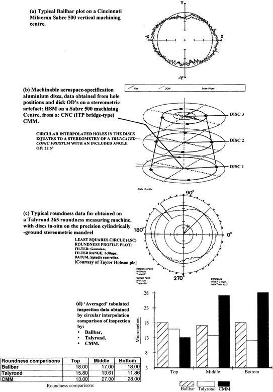

  

  Data obtained from machining a stereometric artefact [Source Smith et al. (2001)]

• the overall combined weight of the mandrel and this disk-assembly was 38 kg; accordingly, this could be considered as a realistic loaded condition for the machine tool to operate under from a practical sense and in this manner, mimic the machine’s operational performance under actual industrial/production conditions.

In order to minimise the milling forces and potential distortion on these machinable disks, HSM was employed, by utilising a spindle-mounted speed increaser¹⁵—see Fig. 5.19. The Speed-increaser utilised a $\varnothing$6 mm high-performance slot drill with quick-flute angle (i.e. being made from Tungsten carbide with PCD multi-coating¹⁶)—allowing the tool to both drill-down 3 mm depth into the disk surface and then scroll-out by circular interpolation milling for the disk’s hole diameters to $\varnothing$10 mm—see Fig. 5.17, i.e. showing a cross-section of the hole’s details in Section on X-X. This HSM was undertaken at 20,000 rev min⁻¹ and notably, the peripheral milling occurred with a circular interpolation feed of 750 mm min⁻¹, with an excess disk stock of 1 mm, meaning that the cutting tool loading was exceedingly small.

5.6.5 Stereometric Artefact —Machined and Metrological Results

After HSM of all of these machinable disks features by circular interpolation on the vertical Machining Centre, the complete artefact with these disks still in situ was carefully removed from the machine tool. It was then automatically inspected for quadrant hole positioning and disk diameters—in the exact same orientation as they were manufactured on the Machining Centre. This metrological inspection was undertaken on an Eastman/ITP four axis bridge-type CNC Coordinate Measuring Machine—see Fig. 5.20. This particular CMM had previously been: Laser-calibrated; thermally error-mapped; then also verified with a Machine Checking Gauge, prior to the artefact undertaking an automated-inspection procedure —enabling this CMM to produce some realistic measurement data. Once CMM data acquisition had been successfully accomplished, the complete artefact assembly was then inspected on a Taylor Hobson Talyrond 265 Roundness Testing Machine within a fully air-conditioned and metrological laboratory environment. Each of these disks were machined for their individual roundness parameter of Least Squares Circle¹⁷ (LSC), as well as the overall disk’s Cylindricity ¹⁸ being assessed, with the averaging of results of three trials, so that the combined results from the Ballbar, CMM and Talyrond are displayed in Fig. 5.21d.

When a comparison is made of these results from the three individual and completely differing metrological inspection procedures, namely: Ballbar, CMM and Talyrond, they exhibit some degree of metrological consistency. For example, a 15 µm variation (i.e. range) is indicated from the top-to-bottom disks, but they also show a mean value of ≈22.7 µm dispersion of results by the CMM. The Talyrond polar plots (i.e. LSC), also produced some consistent roundness results, ranging from <4 µm and having a mean value of ≈14 µm. Conversely, the smallest variability occurred with the Ballbar, producing a range of just 1 µm, with a mean value of ≈17.6 µm—at these three Z-axis heights. Prior to discussing why the CMM results significantly varied from those obtained from the Ballbar and Talyrond, it is worth visually looking at a comparison between the general profile shapes of typical polar plots that were produced by these Ballbar and Talyrond metrology instruments. In Fig. 5.21a (right), a representative polar plot from a Ballbar is shown and likewise in Fig. 5.21c (right) for the Talyrond a typical polar plot is also depicted. Here, their respective profiled shape geometries, in terms of their respective harmonics¹⁹ are remarkably alike, illustrating the same generally similar elliptical shape combined with its identical axis orientation.

Returning to the CMM results only a few data-points are utilised to obtain a measured diameter and its profile, conversely, with both the Ballbar and Talyrond alike, they literally take thousands of actual data-points to obtain the polar plotted profile. When the CMM touches each machinable disk’s profile with its touch-trigger probe, this specific coordinate’s data could have been obtained at the extreme of the elliptical shape, namely at its major and minor diameters—see Fig. 7.6. Such a variation in both the range and discrepancies in the CMM measurements, when compared to the data obtained by either the Ballbar and Talyrond, may possibly account for such diversity—in this instance.

The four $\varnothing$10 mm holes in each disk produced by HSM utilising circular interpolation at their respective quadrant positions (i.e. see Figs. 5.17 and 5.21b), are given in tabulated data form shown in Table 5.3—in terms of their positional accuracy and radial change from their theoretical centres.

Table 5.3 The $\varnothing$10 mm hole positional deviations for the frustum—based upon the three-dimensional Isosceles triangle—in the machinable disks at the four quadrant positions (i.e. from the theoretical), in terms of their actual radial change

From the $\varnothing$10 mm data given in Table 5.3 for the radial change for each disk, for the top, middle, and bottom disks, it was: 46; 45 and 42 µm; respectively, giving a positional uncertainty of 4 µm. Equally, if the difference is considered for the three stacked disks with respect to their angular relationships to each other, at: 0°; 90°; 180° and 270°; then their angular positional changes are: 46; 26; 32 and 49 µm; respectively, giving a positional uncertainty of 23 µm. This general interpolated milled-hole positional uncertainty is still relatively small considering that in this case, each hole’s position is on a different Z-axis plane—spanning a dimensional height of 200 mm. If one considers the grand mean for both cases, then they have a positional uncertainty of just 1 µm, which for a vertical Machining Centre that at the time of testing was three years old, is quite exceptional—having by now, undertaken considerable industrial machinability trials for both the automotive and aerospace industries. Admittedly, this particular machine tool had previously been both Laser-calibrated and Ballbar-diagnostically corrected —thus showing the true relevance of such calibration to resolve and minimise any current machine- and process-errors, which might currently be present within the actual machine tool.

The initial verification work using the Stereometric artefact , has shown—Fig. 5.21—that its overall positional ability when utilised for HSM analysis coupled to accuracy and precision assessment in combination with machine tool diagnostics, has some degree of metrological-success. Here, then, the actual physical weight of this artefact when verifying the machine’s capabilities, would tend to exacerbate any axis geometry and positioning problems for such a machine tool, which provides a realistic measure of the machine tool’s machining and positional performance in-service.

5.7 Small Coordinate Measuring Machine (SCMM)

• Introduction

It is acknowledged that any object greater than a few centimetres in size can be habitually inspected by conventional CMMs, where they can realistically achieve uncertainties of several micrometres. On the other hand, objects that range from a few micrometres down to say, a nanometre, cannot be realistically inspected even on very highly sophisticated CMMs, as in this latter case, the measuring capabilities of nanometrology instrumentation is in effect, mandatory. The problem with any of these nanometrology instruments—which despite their undoubtedly excellent uncertainty performance—is that they cannot measure component parts as large as a few centimetres in size. Likewise at present, there are no 3-D CMMs that can achieve micrometre uncertainties for these complex measurands. So, in order to address this problem, The NPL within the UK, has developed a metrological instrument with a working-volume of 50 mm³, with an uncertainty within the range of: 50–150 nm. At this juncture, this SCMM instrument can be effectively considered as a miniature CMM, which can successfully operate in full 3-D, but can also be programmed in a similar fashion to a conventional CMM, where in use it has achieved some remarkable metrological results .

5.7.1 Small Coordinate Measuring Machine—Design Requirements

With the SCMM situated within its host CMM (i.e. see photograph in Fig. 5.22a, with its schematic design being represented in Fig. 5.23a where the design requirements were essentially based upon three distinct aspects; these were the instrument’s: (i) accuracy (i.e. uncertainty); (ii) working volume (iii) coupled to its traceability . Regarding the instrument’s accuracy, it had to achieve a volumetric uncertainty sufficiently small enough to enable sub-micrometre measurements to be made, when considering the Standards requirements of both ISO 10360 and ISO 14253 .²⁰ Accordingly, at The NPL it set a design target of 50 nm volumetric uncertainty , for a working volume of 50 mm³. Here, the specific requirement was for an accuracy of: ≥1 part in 10⁶, in conjunction with the needs for traceable-metrology. In order to minimise the actual SCMM’s development time, commercial interferometers were employed (i.e. such as the Zygo ZMI2000 range), having 0.31 nm resolution with a linear displacement of 0.005 arcsecond resolution—for the angular rotations. Three such interferometers monitor the six degrees of freedom (i.e. three displacements and three rotations) for the probe system, via direct measurement of these displacements/rotations by three commercial mirrors mounted on the probe assembly (i.e. see Fig. 5.23a)—being termed a reflector cube. The interferometer enables a long range displacement (i.e. 50 mm) of this reflector cube to be measured to nanometric accuracy, having direct traceability via the calibrated laser wavelength. The reflector cube with its accompanying metrology frame—the fixed structure of the SCMM—is manufactured from Invar® for thermal stability .²¹ The probe system has a fully 3-D analogue probe motion, achieved by designing and utilising a low-force probe, having displacement-sensing based on capacitance gauging. These capacitance transducers are calibrated against the interferometers to achieve their respective traceability, with the overall metrology system being schematically displayed in Fig. 5.23a, with details of the probe shown in Fig. 5.23b.

Fig. 5.22

Small coordinate measuring machine (SCMM)—for the highly accurate and precise measurements of miniature components and features [Source Centre of Length Measurement (NPL)]

Fig. 5.23

Schematic details of the ‘small coordinate measuring machine’ (SCMM) [Source Centre of Length Measurement (NPL)/Lewis et al. (2001)]

5.7.2 Small Coordinate Measuring Machine—Interferometers, Autocollimators and Probe Design

In Fig. 5.23c is depicted just one of the SCMM’s three interferometers. These interferometers, as mentioned, measure the displacement and angular rotation—rather than absolute angle. Consequently, at The NPL, it was necessary to incorporate an additional absolute angle measurement system and for this aspect, autocollimators were utilised. Here, each autocollimator utilises a laser beam, which is split from the interferometer’s primary linear measurement beam. These autocollimators act as a four-quadrant photo-detector, which senses two-axis displacements of the beam across the detector’s surface. After calibration, the detectors function as two axis autocollimators, providing absolute angle information that is employed during the alignment and self-calibration of the system. The small beam-splitter directs the beam to one of the autocollimators—as illustrated in Fig. 5.23c. The detector electronics for the autocollimators and counter-cards for the interferometers, are contained remotely from the instrument, preventing any undesirable thermal-related problems.

With this SCMM instrument, the probe is a critical component in its usage, as it actually contacts the object under test—see Fig. 5.23b. Accordingly, the probe must be lightweight—to minimise any dynamic probing-forces , while exhibiting low stiffness, so that any resulting static probe forces are also minimised despite the fact that here, the probe offers no directional bias. Such a probe prevents the miniscule probe’s tip from potentially damaging minute components whilst the probing-process occurs, allowing true 3-D probing—in any arbitrary direction. This probe’s mechanical design was based upon that of Pril et al. (1997); with the capacitance sensing aspect—as utilised by Yang et al. (1998). In Fig. 5.23b, part of the main probe’s system is schematically illustrated, with the probe-flexures being made from beryllium-copper strips, having cross-links produced from tungsten carbide, which are also shown in Fig. 5.23b. The moving portion of this probe assembly has a mass of just ≈370 mg and exhibits a stiffness of ≈10 Nm⁻¹—in all axes. This probe’s working range is 20 µm and if its deflection is 10 µm, this corresponds to an actual probing force of just 0.1 mN. The styli for this probe’s ball-point can be changed, ranging from $\varnothing$0.3 to $\varnothing$1 mm (i.e. this latter stylus is shown in Fig. 5.23b)—depending upon the metrological application. The probe’s sensing elements are three miniature capacitance gauges—also shown in Fig. 5.23b—with each sensor mounted behind a $\varnothing$3 mm aluminium target disc, this being held in situ by the probe’s cross-links. With this probe configuration, any motion of the probe ball causes one, or more of the gaps between the capacitance sensors and its associated target discs to change. Therefore, by elementary trigonometry, this probe motion relates these changes in the three capacitance readings to resolve motion along the conventional three Cartesian axes—see Fig. 5.22b. Probe calibration is achieved by probing along five orthogonal directions, namely: +X; −X; +Y; −Y and −Z; whilst simultaneously monitoring the interferometer outputs. In this manner, the probe’s motion is calibrated with traceability via the laser wavelength. Here, any inhomogeneities of the probe’s motion and the anticipated sphericity errors of the probe tip, can be mapped by measuring against a known reference sphere. This traceable calibration of the analogue probe’s 3-D functions, produces a 3 nm resolution, with a 10 µm range and sub-mN probing force . Of some significant note is that in recent years, this probe’s design has been markedly improved in its fundamental probing potential, see further details of this design configuration in the photograph and its accompanying caption in Fig. 5.22 (top).

Much more could be said concerning the self-calibration and alignment of this SCMM, together with the Host CMM and the control software, but this is more fully described within the supplied references, regarding this SCMM instrument—at the end of the chapter. However, it is worth mentioning the step height standard that has been accurately and precisely measured by this SCMM. Thus, this step height standard was manufactured as a chromium-layer on top of a Zerodur ™–substrate, with the chromium coating providing a uniformly reflective surface. Here, the step’s height is just 200 nm—when it was measured by optical techniques. Consequently, this SCMM could routinely and precisely measure and verify this minute step height, indicating the usefulness and validity of the actual instrument, but also showing its metrological potential across a wide range of miniscule component features on a range of ultra-precision parts.

5.8 A Novel 3-D-Nano Touch Probe—For an Ultra-Precision CMM

• Introduction

During the past few years, the metrological capabilities of CMMs have become very versatile and widespread metrology tools, with today’s CMMs being able to efficiently perform very complex measurement tasks. However, in industry-at-large with the on-going miniaturisation in the fields of mechanical and optical production, there is a new demand for highly accurate geometrical measurements on minute components. Accordingly, any new metrological instrumentation should be designed and developed to have low measurement uncertainties and be able to probe objects with their minute spheres, while utilising very low contact forces. Until the present day, the main limiting factor for the application of CMMs on small components was mainly restricted to the probe-head technology; therefore, new metrological developments are now becoming increasingly urgent for such ultra-precision tasks.

Expressly manufactured for a CMM, the novel 3-D-nano Touch Probe —shown in Fig. 5.24 (top), has exchangeable probes with spheres in the range from: $\varnothing$0.1 to $\varnothing$0.3 mm, exhibiting very low probing forces of: ≤0.5 mN. This actual 3-D probing-device—Fig. 5.24 (top)—is based on parallel kinematics with flexure hinges , being structurally-manufactured out of a single piece of high-grade aluminium. With this probe configuration , all rotational movements of the probing sphere are restricted, thus enabling the remaining potential translational motion to be separated into its X, Y and Z components, each of which are then measured by an inductive sensor. All the probe’s axes have the same orientation with respect to gravity. The probe stiffness is isotropic in nature, with a value of only 20 mN mm⁻¹, while the effective moving mass is ≈7 g. In some early experimental work, with this 3-D-nano Touch Probe , specific and controlled test procedures were performed on a linear measuring machine equipped with a laser interferometer. At this time, the standard deviation of repeated probing-measurements for example, was for the difference between left and right probing on a 5 mm Gauge block and was in the order of 5 nm—see Fig. 5.24 (bottom-right).

Fig. 5.24

A ‘3D-Nanotouch probe’, for an ultra-precision CMM—for the inspection of minute components [courtesy of Mecartex (Switzerland)]

5.8.1 Probing Force and Surface Damage

The point of contact between the probing sphere and the sample test surface should be obtained by measuring probe deflections at several CMM positions. This test permits extrapolation to zero-deflection, where the contact force is zero. This very low probing force is an important factor for a nano-probe, as the actual plastic deformation on say, the indentation of the surface of an aluminium part-feature after probing with a conventional CMM probe—introduces maximal-admissible probing forces for various sphere diameters of 1000 MPa contact pressure in the immediate vicinity of contact. As can be gleaned from the previous statement, these relatively large probing forces of conventional probe systems could create damage to the workpiece’s surface and consequently falsify the measurement result. Typically, if an Atomic Force Microscope (AFM) image of such a plastic surface deformation on an aluminium testpiece was investigated, then when probed with a conventional 3-D touch probe with a sphere of $\varnothing$0.6 mm, this would result in a surface indentation having a 330 nm depth. Whereas, if a probe sphere of $\varnothing$0.1 mm was utilised, but without leaving any permanent surface indentation, the probing-force must be ≈100 times smaller than that with today’s commercial probe systems. This probing-phenomenon means that the probing system stiffness has to be exceedingly small, for example, of the order: 20 mN mm⁻¹, however, still allowing some probe deflection at these low forces. The probing stiffness design and construction criteria, is even more critical with respect to dynamic forces that act when the probing sphere strikes the surface upon its first contact. Hence, the effective moving mass also needs to be as small as possible, to allow reasonable probing approach speeds.

5.8.2 The 3-D-Nano Touch Probe—Constructional Details

This actual 3-D-nano Touch Probe , is based upon parallelograms and flexure hinges having a new kinematic structure that was designed for the probe-head—see Fig. 5.24 (top). This structure leaves the probing sphere with exactly three degrees of freedom . The rotational movements are blocked and the translational motion is separated in its X, Y and Z components, which as previously mentioned, are each measured by an inductive sensor. All axes have the same orientation with respect to gravity and provide identical probing forces in all directions. As a consequence, the main part of the structure is manufactured out of a single piece of aluminium—produced by utilising electro-discharge machining (EDM). For that reason, the most critical and integral part does not need to be assembled. The flexure hinges have a thickness of only 60 µm resulting in an actual stiffness of: 20 mN/mm. Hence, the effective moving mass here is just: 7 g. Due to the low stiffness the deformation caused by gravity needs to be compensated; therefore for this purpose, an adjustable system with permanent magnets was developed.

The measurement range was set to: ±0.2 mm, while the mechanical limits allow a range of: ±0.5 mm; while, the probing element is magnetically attached to the head and positioned by means of three balls in three grooves. The magnetic holding of the probing element allows an easy replacement and acts also as a mechanical fuse. Therefore, the handling of this highly sensitive device remains quite easy to achieve in-service. A small moving mass is important to keep the dynamic contact forces low while maintaining reasonable approach speeds. Some later model calculations have shown that the effective mass (7 g) of the probe is still rather too high. Thus, a small additional mechanical filter element was developed to reduce the effect of dynamic forces. Its stiffness is almost equal in all directions and roughly 100 times higher than that of the probe-head, but it has a very low effective mass, giving a typical approach velocity of: 1 mm/s.

• Experimental Results

The overall performance of this new probe can only be measured on a CMM with equal or better performance than the probe itself. However, at the time of writing this abridged review of the probe, research work was shown to be lacking assessment by an ultra-precision CMM. Consequently, the first experiments with this new 3-D-nano Touch Probe were performed on a linear measuring machine (LMM), being equipped with a laser interferometer. In this manner only probing in a horizontal plane could be made and verified. However, due to the special orientation of the probe coordinate system, all three sensors of the probe-head were involved in these test measurements. Here, this test consisted of probing a known and calibrated 5 mm gauge block on its left and right side—see Fig. 5.24 (bottom-right). The difference between the two points minus the gauge block length is the probe constant, which is essentially the sphere diameter. The repeatability of this probe-constant is an important parameter for a 3-D-nano Touch Probe. In experimental-evaluations, the standard deviation of five such measurements was always in the order of 5 nm. This value includes interferometer noise and machine instability—such as vibration and drift—moreover, for large probe deflections up to 150 µm the linearity of the probe signal was shown to remain very good with this newly designed probe configuration.

• In conclusion

A new 3-D-nano Touch Probe for CMMs with exchangeable probes and low probing forces was developed and as such, a patent has now been filed. This innovative probing-design is based on parallel kinematics with flexure hinges —with the first test measurements recorded being deemed very successful. This actual probe, with its probing forces <0.5 mN, has a repeatability which was in the order of: ≈5 nm. In the near future, for the full characterisation of this probe, it will require a CMM with comparable metrological performance, therefore, it was reportedly planned to incorporate the probe-head into a new ultra-precision CMM at METAS. The primary metrological objective here, being to offer calibration and measurement services for very small/minute parts, up to a size of about 50 mm—at a later date.

5.9 Robotic Arms

• Introduction

Invariably, many Industrial robot arm²² configurations are based upon multi-axes articulated arms. Characteristically, examples can include SCARA robots—often utilised for efficient assembly type-work; while Cartesian coordinate robots, Articulated arm robots (i.e. sometimes termed: Anthropometric robots) as well as Gantry-type robots, will tend to be employed for a wide range of automation/manipulation-tasks. Generally speaking, most types of the current robots can be categorised as a robotic-arm (i.e. ‘manipulator’ in the Standard ISO 8373:2012) . These kinematically configured robots exhibit varying degrees of autonomy, such as:

• some robots are programmed to authentically undertake specific repetitive actions without variation and to a high degree of accuracy. These robotic actions are determined by programmed routines that specify the following: direction; acceleration; velocity; deceleration; and distance of a series of coordinated motions—during such motion;

• while other types of robotic varieties are much more flexible as to the orientation of the object/workpiece on which they are operating, or even the task that has to be performed on the object itself. The robot may even need to identify the object’s geometry/shape, its orientation, etc.—prior to beginning the set programmed-task. Today, some form of Artificial Intelligence (AI) ,²³ is now becoming an increasingly-important factor in any form of automation for these modern industrial robots .

5.9.1 Industrial Robotics—Their Historical Development

Probably the earliest known form of industrial robot , which conforms to the current ISO standard definition, was that invented by ‘Bill’ Griffith P. Taylor back in 1937 and then subsequently published in the: Meccano Magazine (March, 1938). This small and primitive crane-like device was constructed almost entirely by utilising simple Meccano components (i.e. bolted and assembled pre-made toy parts) with each axes being powered by just a small electric motor. With this configuration, five axes of movement were possible, including Grab and Grab-rotation—by the gripper/end-effector. The automation was attained by utilising the well-known technique of punched paper tape—to energise its solenoids, which could then facilitate the movement of the actual crane’s control levers. It was really the applied and fundamental work of George Devol who instigated the first true robotics patents in 1954 (i.e. these being granted in 1961). Back in 1956, the first commercial company to produce an industrial robot of practical use and significant importance was from within the USA, by Unimation, Inc.—this company being founded by George Devol and Joseph F. Engelberger —and here the robot’s design and construction was based upon Devol’s original patents. These early designed and manufactured Unimation robots were also known as Programmable Transfer Machines (PTM’s) —as initially their main working practice was to simply transfer objects from one-point-to-another, typically over distances of up to 4 m.

At this time the robot’s axis motions utilised hydraulic-actuators, which were programmed in joint-coordinates (i.e. the angles of the various joints were stored during a teaching phase and then replayed in actual operation). It has been reported that these robots were positionally accurate to: ≤2.5 mm. Of particular note, is that accuracy here is not usually an appropriate measurement in robotics, as their positional performance is normally evaluated in terms of their repeatability. Somewhat later, Unimation licenced their robotic technology to Kawasaki Heavy Industries (Japan) as well as to GKN (UK) where the actual manufacturing of these robots was carried out. At that time, Unimation’s only major competitor—for a considerable period of time—was from Cincinnati Milacron Inc. (Ohio, USA), although this robotic manufacturing production environment radically changed in the late 1970s, when several of the big Japanese corporations began producing comparable industrial robots. By 1969, Victor Scheinman (at Stanford University, Ca., USA) had invented the so-called Stanford-arm, which was a six axis articulated robot—electrically powered, being designed to permit an arm-solution to its operation. This new robot design and configuration, allowed it to precisely follow arbitrary paths in space—within its working envelope, thus increasing robotic potential usage to the more sophisticated applications such as: assembly; welding; adhesive bonding; also paint-spraying activities, plus many more operations. Later on, Scheinman went on to design a different robotic-arm for the MIT AI Laboratory (USA), where it was termed the MIT-arm. After receiving a fellowship from Unimation to develop his robotic-designs, Scheinman sold these future-designs to Unimation, who then developed them still further, with financial support from General Motors, who later marketed this new robot as the Programmable Universal Machine for Assembly (PUMA)—one version seen here in Fig. 5.25b—with this PUMA’s end-effector being attached to a Partially cubed calibration device .

Fig. 5.25

Calibrating multi-axis robots with artefacts

In Europe during the early 1970s, industrial robotics was quickly developed, typically by such companies as ABB Robotics (Sweden)—see Fig. 5.25a—as well as KUKA Robotics (Germany)—see Fig. 6.15 (top)—who introduced their own robots to the market by 1973. Of note, was that ABB Robotics (formerly known as: ASEA) presented their IRB 6 robot, which was among the world’s first commercially available industrial robots having an all-electric microprocessor-controlled robotic-arm. Likewise, in 1973, KUKA Robotics introduced an industrial robot, known as FAMULUS, which was also an Articulated-robot having six electromechanically driven axes.

In the USA, in the late 1970s, several companies entered this fast-developing robotics-field, such as, General Electric (GE) and General Motors (GM), who then formed joint-ventures with both Japanese FANUC Robotics and with FANUC Ltd. At this time, in the USA, some local startup companies also became involved in robotics, which included both Automatix and Adept Technology, Inc. At the height of the robot-boom (i.e. notably around the mid-1980s) the Westinghouse Electric Corporation had acquired Unimation for $107 million. Later, in 1988, Westinghouse sold Unimation to Stäubli Faverges SCA (a French company) which has manufactured Articulated-robots for wide-ranging industrial and cleanroom applications, and by 2004, Stäubli bought the robotics division of Bosch (Germany). Today, only a few non-Japanese companies have ultimately managed to survive in this highly competitive market; typically just some of the major robotic manufacturers are currently: Adept Technology (USA), Fanuc Corporation (Japan), Stäubli-Unimation (France) and the Swedish/Swiss company ABB (Asea Brown Boveri), plus the highly industrialised German company KUKA Robotics and, in a similar manner, the Italian robotic company Comau.

5.9.2 Defining Robotic Parameters

There are any number of differing methods and techniques to actually define most configurations of industrial robotic arms, some of which might include the:

• number of axes—the minimum of two-axes are necessary to reach any point in a plane; but three axes are required to reach any point in space, so to fully control the orientation of the end of the robotic-arm—termed its wrist—then normally a further three axes are mandatory, these being termed its: yaw; pitch; and roll;

• degrees of freedom—this is usually equivalent to the number of robotic axes;

• working envelope—this is the volumetric region of space that this physical configuration of robotic articulation can effectively reach;

• kinematics —which in robotic-terms, is primarily concerned with the arm’s actual arrangement of its rigid members and joints in the robot, which determines the robot’s conceivable motions.

  NB The actual classes of robot-kinematics will include many differing types, typically these are: Articulated (i.e. Anthropometric); Cartesian; Parallel; SCARA; and Parallel Kinematic Mechanisms (PKMs);

• carrying capacity, or payload—this is how much weight the actual robot can lift, which should also include the weight of its gripper/end-effector;

• speed—this is its dynamic-motion, being concerned with how fast a robot can position the end of its arm.

  NB Speed could be defined in several ways, by terms such as its: angular-speed; linear speed of each axis; or as a compound-speed; but specifically, the speed of the end of the arm when all of its axes are continuously moving;

• acceleration—this is how quickly the arm’s axis can accelerate,

  NB The limiting factor of a robot is that it may not be able to reach its specified maximum speed for movements over just a short distance, or if a complex and variable-path requires frequent changes of direction;

• accuracy—this is how closely a robot can reach its commanded-position.

  NB When the absolute position of the robot is measured and then compared to the commanded-position, this error is a measure of its accuracy; although this accuracy, can be improved with some form of external-sensing, such as when incorporating a vision system, or by Infrared-sensing. Other factors affecting the robotic arm’s accuracy might be the result of varying its speed and position within the working-envelope of these axes with its intended payload;

• repeatability—this term relates to how well, or repeatable, the robot will return to a programmed position,

  NB; however—as mentioned—this repeatability should not be confused with its accuracy. For example, the robotic-arm might be programmed to go to certain X, Y and Z coordinate positions in space, but here, if it gets to only within 1 mm of that position, this would be the robot’s accuracy, although this positional-accuracy can be significantly improved by previous axes calibration—which will now be mentioned in the following section.

5.9.3 Robotic Calibration

The activity concerned with robot calibration, can be defined as, “The process of determining the actual values of kinematic and dynamic parameters of an industrial robot [IR]”. These kinematic parameters designate the robot’s relative position and orientation of its links and joints, while the dynamic parameters describe the arm and joint masses—as well as its internal friction. Accordingly, it seems somewhat obvious that a calibrated robot has a much higher absolute positioning accuracy than an identical uncalibrated robot. Specifically, the real position of the robot’s end-effector would normally correspond much better to the position calculated from the mathematical model of that robot. As a consequence, a robot’s absolute positioning accuracy is, for the most part, relevant in connection with robot exchangeability and for offline programming in any form of precision working-applications. Furthermore, robotic calibration is predominantly concerned with calibrating its tools and the attendant workpieces in its so-called cell calibration configuration, which can help to minimise any potential/occurring inaccuracies and thus, improve the overall production process security.

In SS ISO 9283:2012 ,²⁴ this Standard sets different performance criteria for an industrial robot, where it suggests certain test procedures in order to obtain appropriate robotic parameter values. Here, the significant criteria and probably the most commonly utilised are the robot’s accuracy of pose (AP), together with its repeatability of pose (RP). Robotic repeatability is singularly important when the robot is manually moved towards its command-positions (i.e. during its Teach-In-mode). If, for example, the robot program is generated by the more usual 3-D simulation package (i.e. often termed: Offline programming), then its absolute accuracy is vital. Both of these factors are generally influenced in a negative way by the robot’s kinematic-factors, the joint-offsets and deviations in joint-lengths and angles between the individual robot links being particularly affected.

The problems of robotic errors produced by these pose-measurements can be significantly minimised by what is termed: numerical-optimisation. In the case of a robot’s kinematic calibration, a complete kinematical model of the geometric structure must be developed, whose parameters can then be calculated by mathematical-optimisation. Consequently, the robot’s common system-behaviour can be described with the Vector model function, plus its input- and output-vectors. Here, the robotic-variables of: ‘k’; ‘l’; ‘m’ and ‘n’; with their respective-derivatives, can describe the dimensions of the single-vector spaces. The minimisation of the residual-error ‘r’ for the purpose of identification of the optimal parameter vector ‘p’, occurs, from the difference between its output vectors by utilising the Euclidean-norm. When attempting to solve many of the robot’s kinematical optimisation problems, then the least squares descent techniques can be satisfactorily employed, typically by utilising a Modified quasi-Newton method. These particular and notable robotic analysis techniques are somewhat outside the current textural-remit, but this type of procedure supplies corrected kinematical parameters for the robotic device, which can then be used to update the system variables within the controller, in order to adapt the current robot model to that of its real kinematics . An obvious point worth mentioning here, is that the positioning accuracy of industrial robots varies by: robot manufacturer; its age and usage; the robot-type; plus its axes-configuration. Hence, the magnitude of the robotic-error between the actual and desired positions can range-widely from: ≤0.1 to >2 mm—in certain cases. Consequently, by utilising kinematic calibration, these robotic-errors can invariably be reduced to: ≤1 mm, in most industrial automation cases.

In certain industrial applications, there is something of a trend developing toward the substitution of CNC machine tools and other specialised-machines with that of fully programmable high accuracy/repeatability multi-axes industrial robots . Today, this slowly developing take-up and replacement by robots for certain specified manufacturing tasks, whose accuracy demands can be fulfilled by these calibrated robots, is likely to continue. By the correct application of efficient calibration methods, it is possible with modern industrial robots and more particularly for those of the type with Parallel kinematic manipulators, to achieve an accuracy-of-pose of: ≤0.1 mm. This is expected to endure and increase into the near-future, as a result and in order to improve this robotic-exchangeability, the ability to simplify any offline program activities will enable new and highly precise robotic applications to be successfully utilised.

5.9.4 Robotic Calibration Devices and Techniques

It has been well-documented in the relevant robotic-literature, that ≈97 % of most robot’s positional errors are due to the error in its zero position (i.e. its home-position), which can mean that a full calibration is not always necessary. Accordingly, the technique of remastering can be accomplished by returning the robot to this home position and then simply resetting its encoder values. This simple technique is habitually performed by the robot manufacturer before it is shipped to the end-user. Moreover, the robotic supplier could also recommend that this remastering process is repeated on a regular basis—beginning with its initial installation. There are a considerable number of traditional techniques of programming that involve utilising a robot’s Teach-pendant. Under these circumstances the robot’s end-user does not depend on the accuracy of the manipulator, but simply relies solely on its repeatability. Nonetheless, as these industrial robotic applications become more widely accepted; then, end-users will expect that an industrial robot is both accurate as well as repeatable. After remastering a robot, if it does not provide the end-user with the required accuracy/repeatability for the industrial-application, then it must be recalibrated.

Typically, most effective robotic calibration techniques will compare the actual Teach-point positions, with measurements relating to the tool/gripper and to that of an independent 3-D measuring device/artefact. This comparison enables the robot’s DH-parameters²⁵ within the mathematical model to be modified, so that the actual distance between where the robot assumes it is and, where overall accuracy of the robot’s actual position truly is can then be minimised. This so-called modified model—of the robot’s controller, will depend upon the complexity of the actual calibration technique.

With the advent of advances in Offline programming (OLP) software packages, they now have the capacity to update the robot model within the software—thereby matching the parameters recorded from calibrating the actual robot. In addition, a robot’s calibration can also be accomplished utilising both contact and non-contact probing methods. Invariably the non-contact techniques include utilising either: laser proximity-sensors: beam-breakers; high-resolution cameras; visual servo-ing; or many more techniques. Such non-contact methods can provide the robot with high accuracies, but they have a tendency to be relatively expensive to accomplish. This fact is due to the expense when acquiring this type of calibration equipment, as well as the time required for setup and interfacing with that of the robot controller. This means that the so-called cost drivers in industry ensure that robotic-users have to incorporate much less sophisticated and the somewhat cruder techniques of contact methods for their subsequent robotic calibration. These contact techniques might include the use of a wide range of dummy-parts, compliant-devices, precision-styli or other artefact-based techniques, some of which will now be briefly mentioned below.

• Telescoping Ballbar—For Robotic Calibration

Figure 5.25a depicts a Telescoping Ballbar (i.e. the Ballbar model here is a QC20-W Ballbar produced by the company Renishaw plc; having Bluetooth™ wireless-technology), which is kinematically affixed to a worktable platen at one end and attached to an Articulated arm on a six-axis robot’s end-effector at the other end (i.e. in this case, the robot model was an ABB IRB 1600-6/1.45). This Ballbar’s sensor accuracy at 20 °C is ±0.5 μm—with a measuring range which is limited to just ±1.0 mm. In these calibration trials the end-effector weighed ≈2 kg and was utilised in all of the Ballbar tests that were undertaken. During the robotic-testing procedure, the Ballbar’s circular tests were performed—in both clockwise (CW) and anti-clockwise (ACW) directions, with differing Ballbar-radii, of 100, 150, as well as at 300 mm, with constant feedrates utilising the robot’s Tool Centre Point²⁶ (TCP) operational-mode, with linear-velocities ranging from: 20 to 700 mm s⁻¹. Here, the coordinates of the measurement point (i.e. from the centre of the tool-cup) with respect to the robot’s flange reference-frame, was set at: ≈0; 65; and 149 mm. Prior to beginning any Telescoping Ballbar testing, the robot was initially warmed-up by repeating the actual circular-trajectories for 1 h—from its cold startup (i.e. with the laboratory’s ambient temperature at that time, being 21 °C).

These circular tests were performed on this particular six-axis Articulated arm industrial robot , which highlighted the robot’s servo-dynamic errors that have a significant impact on its contouring-errors, causing out-of-roundness and potentially some large radius sized-errors. These test comparisons with a Telescoping Ballbar, being performed at different TCP rotational speeds, indicated that the robot’s geometric errors are dominant at low TCP speeds, which has a significant impact on its circular contouring errors. Here, the robot’s dynamic errors are present as vibrations, being obviously more dominant at high TCP speeds for small circular -contouring radii, achieving 25 % of the total-error at a TCP-rotation of 700 mm s⁻¹. The robotic results have also indicated that the tested-robot exhibited significant radius size-errors. With these specific Ballbar tests, the research-approach for the modelling and prediction of these radius size-errors was developed, this being based on both the experimental data and statistical testing procedures. Therefore, the developed-model was fitted utilising this experimental data and then its kinematic performance was checked, by comparing the model predictions to additional sets of data, which are dissimilar from those utilised for identification. The Ballbar results from these particular robotic-trials, has demonstrated that the model which was developed was able to predict 98–99 % of its radius size-error.

Therefore in summary, by employing a Telescoping Ballbar, which is an excellent instrument for measuring both the static and dynamic performance of an industrial robot , it thus provided the techniques required towards the verification-information necessary to then potentially calibrate these types of multi-axis robots.

• Robotic Calibration Cube—For Home Positioning

A very common and historically tried-and-tested calibration technique is to locate the robot’s manipulator at its home-position, which usually necessitates that it is positioned with all joint-angles specified to a value of either zero, or at 90°. For large industrial robots, this home-position must be repeatable to ≤0.2 mm, in its cartesian space at the end-point of the robot. Utilising robot-kinematics , the cartesian requirement can be transformed into joint-angle repeatability of just 0.01°. Consequently, to obtain a significant improvement in the robot’s home calibration, this can be found by three separate techniques, these are by:

• 1. relative calibration—this is an expensive process which requires each component in the robotic structure to be defined relative to the previous component. Accuracies from such relative-calibrations can vary to a certain degree, being based upon the accuracy of these robotic components;

• 2. optimal calibration—this utilises a measurement combined with kinematic-models of the robot, to measure numerous positions of the robot—in its envelope, and then correct any errors present in the structure. Accuracy from optimal calibration can vary to some extent, being based upon the robot’s positions and its kinematic model;

• 3. level-based calibration—this calibrating-process employs simple electronic levels (i.e. typically Inclinometers) to easily orientate each component of the robot structure with respect to its angle—this data being read by the Inclinometer.

In order to practically validate the robot’s home-position, a technique of utilising an artefact of an Open-/Partial-cube is conveniently situated (i.e. permanently) on the robot’s flange which is then nested into a kinematic-fixture—situated at another convenient position within the working envelope of the robot (see Fig. 5.25b for a close-up photograph of the robot’s-approach into this kinematic-fixture). Here, within this integrated robotic-cell, it was specifically built to assemble small precision-made reduction-gearboxes, with its interchangeable robotic gripper, which could change all of its robotic tooling from a purpose built tool store, then automatically and accurately assemble these gearbox components and finally bolt them together at completion. The Partial-cube when nesting in the mating fixture (i.e. see Fig. 5.25b) was positioned by the standardised kinematic principle of: 3-2-1-location. That is, the sensors were contact-type strain-gauged devices, with three situated at one internal face, two at another face, with the final face having just one sensor—thereby defining the exact corner datum point (i.e. its defined home position). The kinematic-fixture enabled a closed-loop feedback into the robot’s controller (for linkage positional error adjustment, as necessary). This type of configuration/calibration allowed a true home-position to be established for the robot either during the end-effector’s (i.e. gripper) change-over, or after the completion of the gearbox assembly task. In this manner, the robot’s actual positioning within its volumetric envelope was always known, thus enabling this complex-precision robotic operation to be successfully achieved in-service.

5.10 Parallel Kinematic Mechanism (PKM)—Equator™ Gauge

• Introduction

With the launch of the metrology instrument/artefact known as the Parallel Kinematic Mechanism-based machine (PKM) also being commercially known as the Equator™ Gauge (i.e. see Fig. 5.26), it has been specifically targeted at an industrial user-market said to be potentially worth ≈$3 billion per annum—this model being just the start of a range of related-products. This type of PKM-equipment seems somewhat different to many other types of metrological instruments, because it is neither a CMM, nor a hard-gauging artefact. Such configuration of these PKMs, are most easily explained by stating that when compared to machine tools, or indeed CMMs, they do not have mutually perpendicular axes; furthermore, their axes are not connected in either a serial-chain, nor stacked one-upon-the-other.

Fig. 5.26

The parallel kinematic mechanism-based machine: equator^TM, that can complete in terms of both: speed of operation and versatility, with ‘hard-gauging’ techniques (courtesy of Renishaw plc)

This specific PKM-instrument, has three distinct axes—being either extending, or contracting struts—all of which must be moved in order to position the vertically inclined probe body and its attached stylus, which can be positioned either vertically, or indeed cranked—in any coordinate axis position in: ‘X’; ‘Y’; as well as ‘Z’ axes. For example, the PKM’s platform (see Fig. 5.26a) to which the axes and probe body holding a Renishaw SP25 scanning-probe are connected—is efficiently constrained to remain parallel to this base surface, by means of two struts associated with each axis. These two accurately and precisely positioned struts are there to help prevent the platform from any form of actual twisting, or tilting as the axes are either being extended or contracted (i.e. consequently these struts are necessary for controlling the other—rotational—three degrees-of-freedom, namely the: ‘A’; ‘B’ also ‘C’ rotations; about the instrument’s linear coordinates of its: ‘X’; ‘Y’ and ‘Z’ axes, respectively).

5.10.1 Theory of Operation—Of the PKM

The underlying principle of operation for this Programmable-gauge (see Fig. 5.26) is to utilise flexible bespoke-software to drive this PKM, thus providing versatility for varying product designs. In prior attempts at such flexible-gauging to retool hardware—for example by utilising linear variable differential transformers (LVDTs) —in order to gauge a family of similar parts an instrument’s flexibility tended to be limited and was normally at the cost of significant setup time and lost throughput. This latest Programmable-gauge differentiates itself from many other types of retoolable-gauging, in that it has been reconfigured for completely different part measurements and the metrology process can also be automated, which vastly reduces overall setup time.

On the latest PKM-design the gauging and reconfiguration are simultaneously achieved by moving a single-sensor around the part, in a similar manner to that of a CMM; although here, any particular part-features and tolerance dimensions are programmed and its operation can be totally automated. Traditional hard-gauging has a limited inherent accuracy but has good repeatability (see a typical Receiver-gauge version in Fig. 7.2b). At this present time, the PKM normally has the accuracy obtained by zeroing a Master part’s individual touch-and-scan points to that of the nominal, as if each point was an LVDT in its own right. Unlike that of traditional gauges—which are typically either GO and NO-GO or specified as Pass and Fail—the quantitative dimensional reporting is readily available due to the nature of software-driven inspection. Consequently, by measuring a Master part on a CMM, that CMM’s accuracy and its associated process capability potential, is then simply transferred to this Programmable-gauge through a known set of offsets. Here, the process control possibilities of just one single CMM can be effectively scaled through an arrangement of a series of multiple-versions of these Programmable-gauges and can offer the cost, robustness, and throughput advantages of all types of traditional gauging techniques.

A fundamental property of this PKM-instrument is its closed-loop force-path—as there are no cantilevered-forces within the structure itself as would be the case for an open-loop vertical Machining Centre. These PKMs are therefore very stiff structures indeed, accordingly having a high stiffness-to-weight ratio. For that reason, this Equator™ Gauge can be considered as being thermally neutral—meaning that any structural thermal growth is symmetrical, due to the use of matched materials in its overall construction.

The first product launched in this PKM-range, was the Equator 300 (see Fig. 5.26) having a working envelope of the following dimensions: $\varnothing$300 mm by 150 mm high, which has measurement uncertainty of: ≥±2 µm. This unique PKM-instrument is intended to replace many bespoke hard-gauging applications in a full production industrial environment. The cost of a typical PKM, is financially comparable to that of most hard-gauging systems, but moreover, it is easily and infinitely reconfigurable

The target industrial applications for such a PKM-instrument, are in the medium-to-high volume manufacturing processes, typically found in the automotive sector—for example when measuring conrods/pistons, or for domestic markets—for white goods component inspection, as well as in the medical fields—typically for surgical implants/instruments, also it will find metrological applications in the aerospace industries—more notably for their blade-manufacturing operations. This programmable-gauge has also been envisaged as part of an automated setup, when the parts handling is via productive robot cell configuration—such as if efficient and speedy automatic-offset updates might need to employed. Furthermore, this Equator™ Gauge can also quickly change between differing parts, due to its inherent flexibility obtained from its attached six-stylus probing rack—see Fig. 5.26b.

5.10.2 Calibrating This PKM

Prior to looking in more detail as to how this PKM instrument functions in a metrological application, and being considered as a comparator, its initial calibration must be discussed. In this instance, the term calibration should be more appropriately retitled as Mastering, which can be undertaken in either one, or two specific ways, by means of a:

• 1. Calibrated master part—in this case, the actual master has nominal dimensions for all those component features to be measured;

• 2. Production part—in this instance, where the component’s actual dimensions will be more than likely to deviate from the nominal and as such, it subsequently becomes the accredited Master.

Whichever artefact measurement technique employed for its PKM-verification, the part is firstly measured on a conventional CMM in a temperature-controlled environment (i.e. establishing its actual traceability–to International Standards) with the subsequent CMM’s measurement results output as an ASCII text file for these specific measured data-points. This data is then input into the Equator™ Gauge’s software (i.e. having been developed by Renishaw plc and it is known as MODUS) and then compared against its CAD nominal data (i.e. here in a DMIS-format) which has also been fed into the PKM’s computer. This bespoke-computer software results in the creation of offsets from the nominal, but where the actual measured data-points are not nominal. This PKM-instrument will then measure the Master part—at any temperature—having previously established its position via datum features, thus zeroing the system. After this metrological-action of Remastering, the measurement uncertainty will now be close to 2 µm—for this programmable-gauge. Any subsequent part measurement necessitates that the component parts are placed in virtually the same position—to the nearest millimetre—by locating the parts on a very high accuracy palletised system, which is also available from the supplier. From this time, the actual Remastering needs to occur at periodic intervals—related to process tolerance limits and due to any changes in ambient temperature (i.e. concerning the part’s thermal-growth). Here, it is important to stress that any measurements on this PKM-instrument, are compared data-point-for-data-point with that of the original CMM’s data-points—even when inspecting for any workpiece swept-surfaces. This fact is true, even where CMMs are not utilising Renishaw’s own controller, or are not programmed via the MODUS-software—but they must run the same measurement script. This data-point level of operation is vital, for the metrological instrument to be able to operate correctly.

In summary for this Renishaw Equator™ Gauge , it can be stated that it is a truly Programmable-gauge being constructed upon a parallel kinematic platform with a scanning tactile probe, which makes it a versatile alternative to the majority of conventional Custom-gauging practices, offering inspection of an unprecedented variety of many manufactured high-quality parts. This PKM-system features working-volume in its ‘X’, ‘Y’ and ‘Z’ axes for component part dimensions, which might typically be: $\varnothing$300 mm by 150 mm—having a comparison-uncertainty ±2 µm; with a maximum scanning speed 100 mm s⁻¹; while having a fixturing requirement of ±1 mm; with an electrical supply of single-phase 100–240 V; but here, it does not require any air-supply. This programmable-gauge weighs between 25 and 27 kg, dependent on the model’s arrangement, so it can be deemed as portable—but with some care in its handling. The high-data capture-rates for a part’s rapid form measurement enable thousands of such points to be collected during 3-D-scanning, with the industry-standard Renishaw SP25 probe. Such PKM-measurement results are a reliable form of metrology, which compares remarkably favourably against that of conventional-gauging, enabling an effective technique for that of component form measurement. Every data-point can be utilised for comparative measurement. So, just one PKM-instrument can perform the same function as thousands of DTI’s; LVDT’s; or by that of handheld-instruments. As a consequence, any requirement for Remastering is swiftly performed as when, for example, measuring a production part and it immediately compensates for any possible thermal effects, returning data-collected to the shop floor—being the equivalent to that obtained in a temperature-controlled quality room. This programmable-gauge—as mentioned—can be considered as a cost-effective alternative and invariably should replace equivalent manual measurement, which can greatly increase throughput and reduce scrap-rates, at a fraction of the cost of a custom-gauging system with its related and costly fixturing requirements.

5.11 Articulated Arm CMM (AACMM)

• Introduction

In recent years, there have been many advances in conventional CMM technology, including the development of several portable CMMs. Accordingly, these portable CMMs, can provide many of the benefits of traditional CMMs, but with some added flexibility. Articulated Arm CMMs (AACMM)²⁷—see Fig. 5.27—are also known by the derivative-names of: Portable CMMs (PCMM) or even as Articulated Arm CMMs. These metrology instruments are lightweight and can therefore be utilised virtually anywhere—wherever some form of accurate and precise measurement is demanded. Specifically, the AACMM can be moved to the part for its inspection, hence, the term portable. Under these inspection-circumstances, a controlled environment is unnecessary, as the instrument’s operation is very simple. These portable metrology instruments provide highly accurate and reliable results, with the added-benefit of being robust enough to work in a wide-range of working-environments. Such Portable CMMs are considerably much less expensive to purchase than a conventional, more sophisticated CMM, although this latter-type of CMM metrology equipment, has the distinct advantage of being significantly more precise and indeed accurate in usage.

Fig. 5.27

The archetypal ‘personal coordinate measuring machine’, is normally justified as: a portable, cost-effective and three-dimensional gauge, for speedy assessment of components, etc. (courtesy of FARO Technologies Inc.)

• Rapid Shop Floor Inspection

Invariably, within the modern production shop floor environment when utilising AACMMs there are three significant factors that need to be considered when implementing some form of rapid shop floor inspection, these being for:

• 1. suitable hardware—today, in order to conduct inspection on the shop floor, invariably some form of PCMM is necessary, although here there might be several other metrology options, but the common choice in, say, a small machine shop might be to use an Articulated Arm CMM—equipped with contact probe (see Fig. 5.28, top). It is normal practice to temporarily mount the PCMM on any firm and rigid surface—prior to its use—as shown in Fig. 5.28 (bottom). These lightweight-metrological instruments can be easily transported anywhere within the shop. Such Arms have highly mobile joints that let the Inspector, or even Machinist utilise the equipment—see Figs. 5.27 and 5.28 (top), enabling PCMMs to extend and rotate the measurement-probe into virtually every component feature, such as its: channels; bores; or pockets; or any other types of inspected part-features. Usually these Arms have a reach of between: 0.8 and 2 m, although they are not restricted by the physical size limits that are common with conventional stationary CMMs—making them extremely versatile inspection tools;

  Fig. 5.28

  

  An ‘articulated arm CMM’ prior to use, requires verification against a calibrated artefact [courtesy of the National Physical Laboratory (UK)]

• 2. appropriate software—is a mandatory-requirement, so that it can receive all of the necessary and valid information emanating from inspection by this Arm. In its most basic mode of operation, this bespoke-software will log and report measurement data taken with the Arm. However, the major advantage here is in both the time and efficiency gains, which occur when the software’s full functionality is employed. At this time, the PCCM-software can create prompted-inspection plans, as either datums, or features that are selected while in its teach mode. Moreover, this software will also provide real-time inspection data with visual, on-screen references—to really expedite the overall inspection process, furthermore, it can import a CAD reference model for direct comparison of the manufactured part—to its actual design intent;

• 3. quality specification and inspection plan—the inspection work can be undertaken by referencing a part’s engineering drawings. Although this approach works acceptably, the inspection process becomes much quicker when that measurement data is assigned to a digital reference within the PCMM’s-software.

5.11.1 Articulated Arm CMMs—In More Detail

Most types of Articulated arm CMMs will determine and record the location of its probe in 3-D space and then report the inspection results through suitable-software—as mentioned in Sect. 5.11. As a result and in order to calculate the position of the probe’s tip, the rotational angle of each joint and the length of each segment in the arm must be known—having a radial reach when extended, which typically ranges from: 0.8 to 2 m. The measurement angle of each rotating-joint within the arm is determined by utilising optical rotary-encoders. These high-quality encoders count rotations incrementally, via the detection of accurately spaced lines on a glass grating disc. Once counted, the software then converts these counts into angular-changes. Such Arms—as mentioned—typically have either 6, or 7 axes of rotation, which means the instrument can move throughout a very wide range of physical orientations.

A typical Articulated Arm CMM (AACMM) —is depicted in Fig. 5.27—which can be considered as a high-quality metrology instrument of multi-DoF (i.e. having typically 6 degrees of freedom—6DoF), which is modelled according to the structure of human joints; with a series of linkages being connected by rotating joints. In a comparison with traditional CMMs, the AACMM has the notable-features of small size, lightweight, large measurement range, while being flexible and can be utilised in just about any industrial site. As a consequence, with these unique-advantages the AACMM has been utilised in the fields of: Mould design; Product quality online testing; as well as in the inspection of equipment for maintenance and assembly; plus in situ machine tool component inspection—see Fig. 5.28 (top). At this point, the accuracy of structural parameters is the main influencing-factor to the measurement accuracy of AACMMs, with the structural parameter identification being one of the main measures to improve the accuracy of them. The Arm calibration is an integrated-process of four distinct steps including: (i) modelling; (ii) measurement; (iii) parameter identification; plus its (iv) error-compensation. The selection of the appropriate kinematic model and its calibration model is the premise of calibration of any AACMM and, by subsequent processing of the data of calibration for structural parameter identification achieves the overall calibration of a typical AACMM. In parameter identification, the linearly related structural parameters can result in a so-called Jacobian matrix,²⁸ which is mathematically singular, thus its solution is not the required structural parameters one expects, so the linearly related structural parameters must be determined, before identification.

In order to achieve precise inspection measurements on a part, the touch trigger probes on conventional and stationary CMMs will require controlled speeds when coming in contact with the part’s surface—slowing the approach to any part-feature being measured, which will inevitably increase overall inspection time. Moreover, if this approach is not exactly along the ‘X’, ‘Y’ or ‘Z’ axes, some additional time will be added to the overall process for probe-angle calibration. To precisely establish an accurate probe compensation in association with its spatial orientation when adding either the: fourth-; or fifth-DoF, every probe angle that will be utilised to measure a part must also be calibrated to that of a Master sphere.

The probe-angles on these stationary CMMs can pose a challenge beyond the time necessary to calibrate them. Since additional DoFs are gained with an indexing-head, here the probe-angle is normally adjustable in: 7.5° increments up to 105°—from the vertical. This restriction on the CMM’s probing, can limit potential access to certain part-features. As a consequence, CMMs often need custom-holding fixtures to position and orientate a part, to enable the probe direct-access to a part feature of interest, while for many component parts, multiple fixtures are expensive, but sometimes necessary additions. Conversely, in the case of an Articulated Arm—see Figs. 5.27 and 5.28—the probe approaches the part at any angle without slowing-down as it nears the surface; this action eliminates the probe-angle calibration and the need for custom holding fixtures. For large items and structures requiring inspection, these PCMMs can take on other forms, such as utilising either lasers (see Fig. 5.27, top-right) and that of infrared light. Additionally, the long-range PCMMs can capture measurements up to distances of 100 m, while in many industrial applications Laser-trackers are the most common form of long-range PCMMs, which were previously described and illustrated—see Figs. 2.17, 2.18, 2.19 and 2.20.

5.11.2 Verification of Articulated Arm CMM (AACMM)

In the UK, at The National Physical Laboratory (The NPL) a verification service is offered for Articulate Arm CMMs to the ASME B89 4.22 Standard—this currently being utilised by the majority of these Arm-manufacturers—see Fig. 5.28 (bottom—left and right). Once verified, an Articulated Arm , or Portable CMM, can achieve uncertainties of just a few tens of micrometres and are principally employed in industry for inspecting parts, and more importantly, in many of today’s reverse engineering processes. Unlike traditional inspection equipment, AACMMs allow the measurement system to come to the part being inspected, and as such, these metrological instruments are becoming an increasingly common sight next to assembly lines in high technology factories in a diverse range of industries such as aerospace and automotive, moreover, they are also now being employed in motorsport.

The NPL has become one of the first calibration services within the UK to offer this verification of Articulated arm CMMs to the Internationally recognised and frequently employed ASME B89 4.22 Standard. This particular Standard has become the basis of the manufacturer’s certification, while recently a UK-application has been made for UKAS-accreditation of this calibration service.

Within The NPL, its Engineering Measurement Team has designed and constructed a specialised calibration facility—for these types of PCMM-devices, being based upon the calibration measurements obtained by utilising a highly stable precision-engineered granite structure—weighing around four tonnes (see Fig. 5.28, bottom). This heavy and substantial granite base, supports both the instrument being tested and a pair of calibrated length artefacts manufactured from carbon fibre tubes, these materials being selected for their lightness, stiffness and low coefficient of thermal expansion . These particular tubular-metrological artefacts are 2.4 m long and are positioned and located on kinematic-mounts, bolted onto this stable granite base structure. Each artefact has 19 magnetic-nests defining all possible measurement positions for Articulated Arms that can range in size from about <1 to 4 m in length—see Fig. 5.28 (bottom).

The NPL has manufactured and assembled these calibrated artefacts, including the bonding of these actual nests to the tubes. Following artefact calibration by both a highly sophisticated CMM and a Laser-tracker, each nest was found to have been both set and positioned extremely accurately and precisely. As these AACMMs are invariably utilised on the shop floor, The NPL’s Calibration Service has to be both efficient and fast, to minimise any potential company production downtime. Accordingly, The NPL has written some bespoke-software for guiding the operator through the calibration testing process, enabling them to both record and analyse the measurement data taken and then to automatically generate the necessary and valid certification—for the appropriate verification of their AACMM.

References

Journals and Conference Papers
Beyer, L. & Wulfsberg, J., Practical Robot Calibration with ROSY, in: Robotica, Vol. 22, 505–512, 2004.
Bringmann, B. & Kung, A., A measuring artefact for true 3D machine testing and calibration, Annals of CIRP - Manufacturing Technology, Vol. 54 (1), 471-474, 2005.
Busch, K., Trapet, E. & Wäldele, F., Simple Interim Check of Large Coordinate Measuring Machines, European Prod. Eng’g., Vol. 18, 3-4, 1994.
Chen, W., Xu, X., Dai, P., Chen, Y. & Jiang, Z., Granite Step Gauge: A New Device for Error Measurement on CNC Machine Tools, in: Advanced Materials Research (Volumes 472 - 475), 328-331, Feb. 2012.
Conrad, K.L. & Shiakolas, P.S., Robotic Calibration Issues: Accuracy, Repeatability and Calibration, Proc. of the 8th Mediterranean Conference on Control & Automation (MED 2000), Rio, Patras, GREECE, 17-19 July 2000.
Cox, M.G., Forbes, A.B. & Peggs, G.N., CMM verification and grading, NPL Report CLM 1, National Physical Laboratory, Teddington, UK, 1997.
Cox, M.G., Cross, N.R., Flack, D.R., Forbes, A.B. & Peggs, G.N., Measurement of artefacts using repositioning methods, NPL Report CLM 2, National Physical Laboratory, Teddington, UK, 1998.
Cox, M.G., Forbes, A.B., Harris, P.M., & Peggs, G.N., Determining CMM behaviour from measurements of standard artefacts, NPL Report CISE 15/98, National Physical Laboratory, Teddington, UK, 1998.
De Aquino Silva, J.B., Hocken, R.J., Miller, J.A., Caskey, G.W. & Ramu, P., Approach for uncertainty analysis and error evaluation of four-axis coordinate measuring machines, Int. J. of Adv. Manufact. Tech., Vol. 41 (11-12), 1130-1139, 2009.
Denavit, J. & Hartenberg, R.S., A kinematic notation for lower-pair mechanisms based on matrices, Trans. ASME J. Appl. Mech., Vol. 23, 215–221, 1955.
Elatta, A.Y., Gen, L.P., Zhi, F.L., Daoyuan Y. & Fei, L., An Overview of Robot Calibration, Information Technology Journal, Vol. 3 (1), 74-78, 2004.
Erkan, T., Mayer, R. & Dupont, Y., Reconfigurable uncalibrated 3D ball artefact for five-axis machine volumetric check, Proc. of the 9th Int. Conf. and Exhibition on laser metrology, machine tool, CMM and robotic performance – Proc. of LAMDAMAP 2009, London (UK), June/July 2009.
Erkan, T. & Mayer, J.R.R., A cluster analysis applied to volumetric errors of five-axis machine tools obtained by probing an uncalibrated artefact, Annals of CIRP – Manufacturing Technology, Vol. 59(1), 539-542, 2010.
Erkan, T., Mayer, J.R.R. & Dupont, Y., Volumetric distortion assessment of a five-axis machine by probing a 3D reconfigurable uncalibrated master ball artefact, Precision Eng’g., Vol. 35, 116-125, 2011.
Fang, C. & Butler, D.L., An innovative method for coordinate measuring machine one-dimensional self-calibration with simplified experimental process, Rev Sci Instrum., Vol. 84 (5), May 2013.
Forbes, A.B. & Peggs, G.N., A large reference artefact for CMM verification, Proc. of LAMDAMAP III, Computational Mechanics Pub., 393-400, 1997.
Hamana, H., Tominaga, M., Ozaki, M. & Furutani, R., Calibration of Articulated Arm Coordinate Measuring Machine Considering Measuring Posture, Int. J. of Automation Technology, Vol.5 (2) 109-114, 2011.
Hope, A.D. & Blackshaw, D.M.S., The application of artefacts and lasers to perform verification of coordinate measuring machines, Proc. of LAMDAMAP V, WIT Press., 117-126, 2001.
Knapp, W., Tschudi, U. & Bucher, A., Comparison of different artefacts for interim coordinate-measuring machine checking: a report from the Swiss Standards Committee, Precision Eng’g., Vol. 13 (4), 277-291, 1991.
Knapp, W., Interim Checks for Machine Tools, Proc. of LAMDAMAP III, Computational Mechanics Pub., 161-168, 1997.
Knebel, R., Scanning for better results [Concerning probing-points for roundness on a CMM], 76-78, Nov. 1999.
Kruth, J-P., Zhou, L., Van den Bergh, C. & Vanherck, P., A Method for Squareness Error Verification on a Coordinate Measuring Machine, Int. J. of Adv. Manuf. Technol., Vol. 21 (10-11), 874-878, July 2003.
Kunzmann, H., Trapet, E. & Waeldele, F., A Uniform Concept for Calibration, Acceptance Test, and Periodic Inspection of CMMs using Reference Objects, Annals of CIRP, Vol. 39(1), 561-564, 1990.
Lewis, A., Oldfield, S. & Peggs, G.N., The NPL Small CMM – 3-D measurement of small features, Proc. of LAMDAMAP V, WIT Press, 197-207, 2001.
Liu, P. & Fu, J., Modeling method for mechanism configuration of the articulated industrial robot, Advanced Materials Research, Vol. 694-7, 1696-1699, May 2013.
Mao, X., Hanmin Shi, B.L., Xi Li, H.L. & Li, P., Error measurement and assemble error correction of a 3D-step-gauge, Frontiers of Mechanical Engineering in China, Vol. 2 (4), 388-393, Oct. 2007.
Mutilba, U., Kortaberria, G., Olarra, A., Gutiérrez, A., Gomez-Acedo, E. & Zubieta, M., Performance Calibration of Articulated Arm Coordinate Measuring Machine, Procedia Engineering, Vol. 63, 720–727, 2013.
Nardelli, V.C. & Donatell, G.C., A Simple Solution to Interim Check of Coordinate Measuring Machines, XVIII IMEKO World Congress - Metrology for a Sustainable Development Rio de Janeiro, Brazil, Sept. 2006.
Nguyen, H-N., Zhou, J. & Kang, H-J., A new Full Pose Measurement Method for Robot Calibration, in: Sensors (Basel), Vol. 37 (7), 9132-9147, July 2013.
Nubiola, A, & Bonev, I.A., Absolute robot calibration with a single telescoping ballbar, Precision Engineering, Vol. 38 (3), 472-480, 2014.
Omari, M., Ajao, D., Kampmann, G.G. & Schmadel, I., Machine Tool Accuracy Quick Check in Automotive Tool and Die Manufacture, Annals of the CIRP, Vol. 56 (1), 2007.
Osawa1, S., Sato, O. & Takatsuji, T., Project for supporting Japanese local public metrology institutes in the field of a coordi-nate metrology, The 10th International Symposium of Measurement Technology and Intelligent Instruments, Japan, June 29 to July 2011.
Pahk, H. & Kim, J., Development of computer aided calibration module for CMMs and machine tools using a compensated step gauge, KSME Journal, Vol. 7(2), 158-164, June 1993.
Peggs, G.N., Creating a Standards Infrastructure for Coordinate Measurement Technology in the UK, Annals of CIRP, Vol. 38(1), 521-523, 1989.
Peggs, G.N., Developing Standards for CMMs, Quality Today, S1-S3, 1998.
Pril, W.O., Struik, K.G. & Schellekens, P.H.J., Development of 2D probing system with nanometer resolution, Proc. of 16th ASPE, 438-442, 1997.
Quality Digest, The New Face of Automation - High-speed, comparative gauging system makes cell integration possible [Parallel Kinematic Mechanism], Oct. 2013.
Ran, H., Liu, S. & Zhang, H., Articulated Arm Length Calibration for Cantilever Coordinate Measuring Machine, Applied Mechanics & Materials, Vol. 333-5, 77-80, 2013.
Ruijl, T., Franse, J. & van Eijk, J., Ultra precision CMM aiming for the ultimate concept, Proc. of 2nd Euspen Int. Conf. (Turin, Italy), 234-237, May 2001.
Russell, S.J. & Norvig, P., Artificial Intelligence: A Modern Approach (2nd Ed.), Upper Saddle River, New Jersey: Prentice Hall, 2003.
Sagar, P., When the last several microns count, S12-S14, July 1998.
Saundry, L., Standards and traceability, Quality Today, S38-S40, July, 1998.
Schuetz, G., Harmonic Analysis [Concerning machined roundness of components], Modern Machine Shop, Jan. 2007.
Scott, P., Fundaments of measurement for testing software in computationally-intensive metrology, Proc. of LAMDAMAP XI, The University of Huddersfield (UK), 2015.
Sims, C., Hope, A.D, Smith, G.T. & Gull, M., Correlation of machine tool and CMM accuracy and precision, Proc. of LAMDAMAP IV, WIT Press, 389-402, 1999.
Singh, J., Hughes, M. & Petzing, J.N., Investigating the volumetric performance of multi-axis measurement arms, Proc. of LAMDAMAP VI, WIT Press, 131-139, 2003.
Slamani, M., Nubiola, A. & Bonev, I., Assessment of the Positioning Performance of an Industrial Robot, Industrial Robot, Vol. 39 (1), 57–68, 2012.
Slamani, M., Nubiola, A. & Bonev, I., Effect of Servo Systems on the Contouring Errors in Industrial Robots, Trans. of the Canadian Soc. for Mech. Eng’g., Vol. 36 (1), 83-96, 2012.
Smith, G.T., Sims, C., Hope, A.D. & Gull, M., A stereometric artefact for volumetric calibration of machining centres, Proc. of LAMDAMAP V, WIT Press, 51-58, 2001.
Sumiya, H. & Irifune, T., Microstructure and Mechanical Properties of High- Hardness Nano-Polycrystalline Diamonds, SEI Technical Review, No. 66, 85-91, April 2008.
Tagiyev, N. & Alizade, R., A Forward and Reverse Displacement Analysis for a 6-DOF In-Parallel Manipulator, Mech. Mach. Theory, Vol. 29 (1), 115–124, 1994.
Takeshima, H. & Ihara, Y., Finished Test Piece Example for Five axis Machining Centers, Proc. of the 5th Int. Conf. on Leading Edge Manufacturing in 21st century (LEM21), 123-126, 2009.
Trapet, E. & Franke, M., The Ball Cube Method for CMM Interim Checks, Workshop on Traceability of Coordinate Measuring Machines, PTB Braunschweig, 9 & 10 Oct. 1997.
Trevelyan, J. P., Robot Calibration with a Kalman Filter, Presentation at Int. Conf. on Advanced Robotics and Computer Vision (ICARCV96), Singapore 1996.
Wang, X.Y., Liu, S.G., Zhang, G.X., Wang, B. & Guo, L.F., Calibration Technology of the Articulated Arm Flexible CMM, Engineering Materials, Vol. 318-2, 161-164, 2008.
Weckenmann, A. & Petrovic, N., Conceptualization of Comparative Measurements of Artefacts Intended for Inspection of CMM Length Measuring Capability, 4th Research/Expert Conf. with Int. Participations, ‘QUALITY 2005’, Fojnica, B&H, Nov., 2005.
Woody, B.A., Smith, K.S., Hocken, R.J. & Miller, J.A., A technique for enhancing machine tool accuracy by transferring the metrology reference from the machine tool to the workpiece, J. of Manufact. Science and Eng’g., Trans. of ASME, Vol. 129 (3), 636-643, 2007.
Yang, S., Li, S., Kaiser, M.J. & Kwun, F.H., A probe for the measurement of diameters and form error of small holes, Meas. Sci. Technol., Vol. 9, 1365-1368, 1998.
Ziegert, J. & Mize, C., The laser ball bar: a new instrument for machine tool metrology, Precision Engineering, Vol.16 (4), 259-267, 1994.
Books, Booklets and Guides
* The actual researchers involved from their work at various research organisations.
Alexander, W.O., Davies, G.J., Reynolds, K.A. & Bradbury, E.J., Essential Metallurgy for Engineers, Van Nostrand Reinhold Pub. (UK), 1985.
ANSI/ASME B89: Methods for Performance Evaluation of Coordinate Measuring Machines, The American Society for Mechanical Engineering, New York, 1990.
ANSI/ASME B5.54:1992, Methods for Performance Evaluation of Computer Numerically Controlled Machining Centers, The American Society of Mechanical Engineers, New York, 1992.
ASME B89.4.22-2004: Methods for performance evaluation of articulated arm coordinate measuring machines, 2004.
Boeing, D38553-4:1999, Testing and Acceptance - 1999, BCAG Equipment Design and Asset Acquisition Standards (EDAAS), 1999.
Bosch, J.A., Coordinate Measuring Machines and Systems, Marcel Dekker, INC. New York, 1995.
Bossoni, S., Geometric and Dynamic Evaluation and Optimization of Machining Centers, for the degree of: Dr. sc. ETH Zürich, Diss. ETH No. 18382, 2009.
Bossoni, S., Geometric and Dynamic Evaluation and Optimization of Machining Centers, Zürcher Schriften zur Produktionstechnik, Fortschritt-Berichte VDI Reihe 2 Nr. 672. Düsseldorf: VDI-Verlag, 2009.
Buice, E.S., Implementation of Dynamic Positioning Machine for nano-scale Engineering, PhD Dissertation, The University of North Carolina at Charlotte, 2007.
Butler, B.P., Forbes, A.B. & Kenward, P.K., Position Calibration Software: Fortran implementation of algorithms to determine frame of reference from measurements of registration points, NPL Report CISE 14/98, National Physical Laboratory, Teddington, UK, 1998.
Callister, Jr., W.D., Materials Science and Engineering – An Introduction (6th Ed.), John Wiley & Sons, Inc., 2003.
Colestock, H., Industrial Robotics – Selection, Design& Maintenance, McGraw-Hill Pub., 2005.
Corta, R., Cox, M.G., Cross, N.R., Dotson, J.R., Flack, D.R., Forbes, A.B., O’Donnell, J., Peggs, G.N. & Prieto, E., A large reference artefact for CMM verification, NPL Report CLM 6 (PDB: 1301), May 1998.
Cubero, S. (Ed.), Industrial Robotics: Theory, Modelling and Control, Pub. by: Pro Literatur Verlag, Germany / ARS, Austria, Dec. 2006.
Dagnall, H., Let’s Talk Roundness, (3rd Ed.), Taylor Hobson Pub., Nov. 1996.
Flack, D.R., Measurement Good Practice Guide No. 42 - CMM Verification, National Physical Laboratory Pub.,.
Forbes, A.B., Least squares best fit geometric elements, NPL Report DITC 140/89,National Physical Laboratory, Teddington, UK, 1998.
Hazewinkel, M. (Ed.), ‘Jacobian’ - Encyclopedia of Mathematics, Springer Pub., 2001.
ISO 10791-7:1998(E), Test conditions for machining centres - Part 7: Accuracy of a finished test piece, International Standard, International Organization for Standardization, Geneva, Switzerland, 1998.
ISO 9283 - Manipulating industrial robots. Performance criteria and related test methods, (Geneva) 1998.
JIS B 7440-1987: Test Code for Accuracy of Coordinate Measuring Machines, by: Japanese Standards Association.
Koba-step: Precision Step gauge, plus data-analysis software – equals - a complete system for monitoring coordinate measuring machines, by: Kolb & Baumann GmbH & Co., (DE-63741 Aschaffenburg, Daimlerstr. 24, Germany), 2009.
Luger, G. & Stubblefield, W., Artificial Intelligence: Structures and Strategies for Complex Problem Solving (5th Ed.), The Benjamin/Cummings Pub. Co., Inc., 2004.
Meli, F., Bieri, M., Thalmann, R., Fracheboud, M.*, Breguet, J-M.*, Clavel, R.* & Bottinelli, S.**, Novel 3D analogue probe with a small sphere and low measurement force, Swiss Federal Office of Metrology and Accreditation (METAS)/**Mecartex/*Institut de Production et Robotique (IPR-LSRO), Switzerland, 2014.
NAS 979:1969, Uniform Cutting Tests - NAS Series Metal Cutting Specification, Aerospace Industries Association of America, Inc. (AIA), 1969.
NCG 2005 - NCG-Prufwerkstuck fur die 5-Achs-Simultan-Frasbearbeitung, [NCG test piece for 5-axis-simulataneous milling], NC-Gesellschaft, 2005.
NF E11-150: Accuracy of Coordinate Measuring Machines, France, 1986.
Paul, R., Robot manipulators: mathematics, programming, and control: the computer control of robot manipulators. Cambridge, MA: MIT Press, 1981.
Quinn, T., From Artefacts to Atoms: The BIPM and the Search for Ultimate Measurement Standards, Oxford University Press, 2012.
Smith, G.T., Industrial Metrology – Surfaces and Roundness, Springer Verlag Pub., 2002.
Smith, G.T., Cutting Tool Technology – Industrial Handbook, Springer Verlag Pub., 2008.
Thelning, K-E., Steel and its Heat Treatment – Bofors Handbook, Butterworths Pub., 1975.
VDI/VDE 2617 – Parts 1 to 5: Accuracy of Coordinate Measuring Machines, Dusseldorf, Germany, 1986-1991.
VDI/VDE 2617 Part 9: Acceptance and reverification test for articulated arm measuring machines, 2009.
Author information
Authors and Affiliations
Corresponding author
Rights and permissions
Copyright information
© 2016 Springer International Publishing Switzerland
About this chapter
Cite this chapter
Smith, G.T. (2016). Artefacts for Machine Verification. In: Machine Tool Metrology . Springer, Cham. https://doi.org/10.1007/978-3-319-25109-7_5
Download citation
DOI: https://doi.org/10.1007/978-3-319-25109-7_5
Published:
Publisher Name: Springer, Cham
Print ISBN: 978-3-319-25107-3
Online ISBN: 978-3-319-25109-7
eBook Packages: EngineeringEngineering (R0)