The Idris Programming Language

Abstract

Types describe a program’s meaning. Dependent types, which allow types to be predicated on values, allow a program to be given a more precise type, and thus a more precise meaning. Typechecking amounts to verifying that the implementation of a program matches its intended meaning. In this tutorial, I will describe Idris, a pure functional programming language with dependent types, and show how it may be used to develop verified embedded domain specific languages (EDSLs). Idris has several features intended to support EDSL development, including syntax extensions, overloadable binders and implicit conversions. I will describe how these features, along with dependent types, can be used to capture important functional and extra-functional properties of programs, how resources such as file handles and network protocols may be managed through EDSLs, and finally describe a general framework for programming and reasoning about side-effects, implemented as an embedded DSL.

These keywords were added by machine and not by the authors. This process is experimental and the keywords may be updated as the learning algorithm improves.

1 Introduction

In conventional programming languages, there is a clear distinction between types and values. For example, in Haskell [13], the following are types, representing integers, characters, lists of characters, and lists of any value respectively:

• Int, Char, [Char], [a]

Correspondingly, the following values are examples of inhabitants of those types:

• 42, ’a’, "Hello world!", [2,3,4,5,6]

In a language with dependent types, however, the distinction is less clear. Dependent types allow types to “depend” on values — in other words, types are a first class language construct and can be manipulated like any other value. A canonical first example is the type of lists of a specific length¹, Vect n a, where a is the element type and n is the length of the list and can be an arbitrary term.

When types can contain values, and where those values describe properties (e.g. the length of a list) the type of a function can describe some of its own properties. For example, concatenating two lists has the property that the resulting list’s length is the sum of the lengths of the two input lists. We can therefore give the following type to the app function, which concatenates vectors:

This tutorial introduces Idris, a general purpose functional programming language with dependent types, and in particular how to use Idris to implement Embedded Domain Specific Languages (EDSLs). It includes a brief introduction to the most important features of the language for EDSL development, and is aimed at readers already familiar with a functional language such as Haskell or OCaml. In particular, a certain amount of familiarity with Haskell syntax is assumed, although most concepts will at least be explained briefly.

1.1 Outline

The tutorial is organised as follows:

• This Section describes how to download and install Idris and build an introductory program.

• Section 2 introduces the fundamental features of the language: primitive types, and how to define types and functions.

• Section 3 describes type classes in Idris and gives two specific examples, Monad and Applicative.

• Section 4 describes dependent pattern matching, in particular views, which give a means of abstracting over pattern matching.

• Section 5 introduces proofs and theorem proving in Idris, and introduces provisional definitions, which are pattern definitions which require additional proof obligations.

• Section 6 gives a first example of EDSL implementation, a well-typed interpreter

• Section 7 describes how Idris provides support for interactive program development, and in particular how this is incorporated into text editors.

• Section 8 introduces syntactic support for EDSL implementation.

• Section 9 gives an extending example of an EDSL, which supports resource aware programming.

• Section 10 describes how Idris supports side-effecting and stateful programs with system interaction, by using an EDSL.

• Finally, Sect. 11 concludes and provides references to further reading.

Many of these sections (Sects. 2, 4, 5, 7, 8 and 10) end with exercises to reinforce your understanding. The tutorial includes several examples, which have been tested with Idris version 0.9.14. The files are available in the Idris distribution, so that you can try them out easily². However, it is strongly recommended that you type them in yourself, rather than simply loading and reading them.

1.2 Downloading and Installing

Idris requires an up to date Haskell Platform³. Once this is installed, Idris can be installed with the following commands:

This will install the latest version released on Hackage, along with any dependencies. If, however, you would like the most up to date development version, you can find it on GitHub at https://github.com/idris-lang/Idris-dev. You can also find up to date download instructions at http://idris-lang.org/download.

To check that installation has succeeded, and to write your first Idris program, create a file called “hello.idr” containing the following text:

We will explain the details of how this program works later. For the moment, you can compile the program to an executable by entering idris hello.idr -o hello at the shell prompt. This will create an executable called hello, which you can run:

Note that the indicates the shell prompt! Some useful options to the idris command are:

• -o prog to compile to an executable called prog.

• –check type check the file and its dependencies without starting the interactive environment.

• –help display usage summary and command line options.

1.3 The Interactive Environment

Entering idris at the shell prompt starts up the interactive environment. You should see something like Listing 1.

This gives a ghci-style interface which allows evaluation of expressions, as well as type checking expressions, theorem proving, compilation, editing and various other operations. :? gives a list of supported commands. Listing 2 shows an example run in which hello.idr is loaded, the type of main is checked and then the program is compiled to the executable hello.

Type checking a file, if successful, creates a bytecode version of the file (in this case hello.ibc) to speed up loading in future. The bytecode is regenerated on reloading if the source file changes.

2 Types and Functions

2.1 Primitive Types

Idris defines several primitive types: Int, Integer and Float for numeric operations, Char and String for text manipulation, and Ptr which represents foreign pointers. There are also several data types declared in the library, including Bool, with values True and False. We can declare some constants with these types. Enter the following into a file prims.idr and load it into the Idris interactive environment by typing idris prims.idr:

An Idris file consists of a module declaration (here module prims) followed by an optional list of imports (none here, however Idris programs can consist of several modules, each of which has its own namespace) and a collection of declarations and definitions. The order of definitions is significant — functions and data types must be defined before use. Each definition must have a type declaration (here, x : Int, foo : String, etc.). Indentation is significant — a new declaration begins at the same level of indentation as the preceding declaration. Alternatively, declarations may be terminated with a semicolon.

A library module prelude is automatically imported by every Idris program, including facilities for IO, arithmetic, data structures and various common functions. The prelude defines several arithmetic and comparison operators, which we can use at the prompt. Evaluating things at the prompt gives an answer, and the type of the answer. For example:

All of the usual arithmetic and comparison operators are defined for the primitive types (e.g. == above checks for equality). They are overloaded using type classes, as we will discuss in Sect. 3 and can be extended to work on user defined types. Boolean expressions can be tested with the if...then...else construct:

2.2 Data Types

Data types are defined in a similar way to Haskell data types, with a similar syntax. Natural numbers and lists, for example, can be declared as follows:

The above declarations are taken from the standard library. Unary natural numbers can be either zero (Z), or the successor of another natural number (S k). Lists can either be empty (Nil) or a value added to the front of another list (x :: xs). In the declaration for List, we used an infix operator ::. New operators such as this can be added using a fixity declaration, as follows:

Functions, data constructors and type constructors may all be given infix operators as names. They may be used in prefix form if enclosed in brackets, e.g. (::). Infix operators can use any of the symbols:

2.3 Functions

Functions are implemented by pattern matching, again using a similar syntax to Haskell. The main difference is that Idris requires type declarations for all functions, and that Idris uses a single colon : (rather than Haskell’s double colon ::). Some natural number arithmetic functions can be defined as follows, again taken from the standard library:

The standard arithmetic operators + and * are also overloaded for use by Nat, and are implemented using the above functions. Unlike Haskell, there is no restriction on whether types and function names must begin with a capital letter or not. Function names (plus and mult above), data constructors (Z, S, Nil and ::) and type constructors (Nat and List) are all part of the same namespace. As a result, it is not possible to use the same name for a type and data constructor.

Like arithmetic operations, integer literals are also overloaded using type classes, meaning that we can test these functions as follows:

Aside: It is natural to ask why we have unary natural numbers when our computers have integer arithmetic built in to their CPU. The reason is primarily that unary numbers have a convenient structure which is easy to reason about, and easy to relate to other data structures, as we will see later. Nevertheless, we do not want this convenience to be at the expense of efficiency. Idris knows about the relationship between Nat (and similarly structured types) and numbers, so optimises the representation and functions such as plus and mult.

where Clauses. Functions can also be defined locally using where clauses. For example, to define a function which reverses a list, we can use an auxiliary function which accumulates the new, reversed list, and which does not need to be visible globally:

Indentation is significant — functions in the where block must be indented further than the outer function.

Scope. Any names which are visible in the outer scope are also visible in the where clause (unless they have been redefined, such as xs here). A name which appears only in the type will be in scope in the where clause if it is a parameter to one of the types, i.e. it is fixed across the entire structure.

As well as functions, where blocks can include local data declarations, such as the following where MyLT is not accessible outside the definition of foo:

In general, functions defined in a where clause need a type declaration just like any top level function. However, the type declaration for a function f can be omitted if:

• f appears in the right hand side of the top level definition

• The type of f can be completely determined from its first application

So, for example, the following definitions are legal:

2.4 Dependent Types

Vectors. A standard example of a dependent type is the type of “lists with length”, conventionally called vectors in the dependent type literature. In the Idris library, vectors are declared as follows:

Note that we have used the same constructor names as for List. Ad-hoc name overloading such as this is accepted by Idris, provided that the names are declared in different namespaces (in practice, normally in different modules). Ambiguous constructor names can normally be resolved from context.

This declares a family of types, and so the form of the declaration is rather different from the simple type declarations earlier. We explicitly state the type of the type constructor Vect—it takes a Nat and a type as an argument, where Type stands for the type of types. We say that Vect is indexed over Nat and parameterised by Type. Each constructor targets a different part of the family of types. Nil can only be used to construct vectors with zero length, and :: to construct vectors with non-zero length. In the type of ::, we state explicitly that an element of type a and a tail of type Vect k a (i.e., a vector of length k) combine to make a vector of length S k.

We can define functions on dependent types such as Vect in the same way as on simple types such as List and Nat above, by pattern matching. The type of a function over Vect will describe what happens to the lengths of the vectors involved. For example, ++, defined in the library, appends two Vects:

The type of (++) states that the resulting vector’s length will be the sum of the input lengths. If we get the definition wrong in such a way that this does not hold, Idris will not accept the definition. For example:

This error message suggests that there is a length mismatch between two vectors — we needed a vector of length m, but provided a vector of length n.

Finite Sets. Finite sets, as the name suggests, are sets with a finite number of elements. They are declared as follows (again, in the prelude):

For all n : Nat, Fin n is a type containing exactly n possible values: fZ is the first element of a finite set with S k elements, indexed by zero; fS n is the n+1th element of a finite set with S k elements. Fin is indexed by a Nat, which represents the number of elements in the set. Obviously we can’t construct an element of an empty set, so neither constructor targets Fin Z.

A useful application of the Fin family is to represent bounded natural numbers. Since the first n natural numbers form a finite set of n elements, we can treat Fin n as the set of natural numbers bounded by n.

For example, the following function which looks up an element in a Vect, by a bounded index given as a Fin n, is defined in the prelude:

This function looks up a value at a given location in a vector. The location is bounded by the length of the vector (n in each case), so there is no need for a run-time bounds check. The type checker guarantees that the location is no larger than the length of the vector.

Note also that there is no case for Nil here. This is because it is impossible. Since there is no element of Fin Z, and the location is a Fin n, then n can not be Z. As a result, attempting to look up an element in an empty vector would give a compile time type error, since it would force n to be Z.

Implicit Arguments. Let us take a closer look at the type of index:

It takes two arguments, an element of the finite set of n elements, and a vector with n elements of type a. But there are also two names, n and a, which are not declared explicitly. These are implicit arguments to index. We could also write the type of index as:

Implicit arguments, given in braces {} in the type declaration, are not given in applications of index; their values can be inferred from the types of the Fin n and Vect n a arguments. Any name with a lower case initial letter which appears as a parameter or index in a type declaration, but which is otherwise free, will be automatically bound as an implicit argument. Implicit arguments can still be given explicitly in applications, using {a=value} and {n=value}, for example:

In fact, any argument, implicit or explicit, may be given a name. We could have declared the type of index as:

It is a matter of taste whether you want to do this — sometimes it can help document a function by making the purpose of an argument more clear.

“using” Notation. Sometimes it is useful to provide types of implicit arguments, particularly where there is a dependency ordering, or where the implicit arguments themselves have dependencies. For example, we may wish to state the types of the implicit arguments in the following definition, which defines a predicate on vectors:

An instance of Elem x xs states that x is an element of xs. We can construct such a predicate if the required element is Here, at the head of the list, or There, in the tail of the list. For example:

If the same implicit arguments are being used several times, it can make a definition difficult to read. To avoid this problem, a using block gives the types and ordering of any implicit arguments which can appear within the block:

Note: Declaration Order and mutual Blocks. In general, functions and data types must be declared before use, since dependent types allow functions to appear as part of types, and their reduction behaviour to affect type checking. However, this restriction can be relaxed by using a mutual block, which allows data types and functions to be defined simultaneously:

In a mutual block, the Idris type checker will first check all of the type declarations in the block, then the function bodies. As a result, none of the function types can depend on the reduction behaviour of any of the functions in the block.

2.5 I/O

Computer programs are of little use if they do not interact with the user or the system in some way. The difficulty in a pure language such as Idris — that is, a language where expressions do not have side-effects — is that I/O is inherently side-effecting. Therefore in Idris, such interactions are encapsulated in the type IO:

We’ll leave the definition of IO abstract, but effectively it describes what the I/O operations to be executed are, rather than how to execute them. The resulting operations are executed externally, by the run-time system. We’ve already seen one IO program:

The type of putStrLn explains that it takes a string, and returns an element of the unit type () via an I/O action. There is a variant putStr which outputs a string without a newline:

We can also read strings from user input:

A number of other I/O operations are defined in the prelude, for example for reading and writing files, including:

2.6 “do” Notation

I/O programs will typically need to sequence actions, feeding the output of one computation into the input of the next. IO is an abstract type, however, so we can’t access the result of a computation directly. Instead, we sequence operations with do notation:

The syntax $\mathtt x <{-} ~\mathtt{iovalue}$ executes the I/O operation iovalue, of type IO a, and puts the result, of type a, into the variable x. In this case, getLine returns an IO String, so name has type String. Indentation is significant — each statement in the do block must begin in the same column. The return operation allows us to inject a value directly into an IO operation:

As we will see later, do notation is more general than this, and can be overloaded.

2.7 Laziness

Normally, arguments to functions are evaluated before the function itself (that is, Idris uses eager evaluation). However, consider the following function:

This function uses one of the t or e arguments, but not both (in fact, this is used to implement the if...then...else construct as we will see later. We would prefer if only the argument which was used was evaluated. To achieve this, Idris provides a Lazy data type, which allows evaluation to be suspended:

A value of type Lazy a is unevaluated until it is forced by Force. The Idris type checker knows about the Lazy type, and inserts conversions where necessary between Lazy a and a, and vice versa. We can therefore write boolCase as follows, without any explicit use of Force or Delay:

2.8 Useful Data Types

The Idris prelude includes a number of useful data types and library functions (see the lib/ directory in the distribution). The functions described here are imported automatically by every Idris program, as part of Prelude.idr in the prelude package.

List and Vect. We have already seen the List and Vect data types:

Note that the constructor names are the same for each — constructor names (in fact, names in general) can be overloaded, provided that they are declared in different namespaces (in practice, typically different modules), and will be resolved according to their type. As syntactic sugar, any type with the constructor names Nil and :: can be written in list form. For example:

• [] means Nil

• [1,2,3] means 1 :: 2 :: 3 :: Nil

The library also defines a number of functions for manipulating these types. map is overloaded both for List and Vect and applies a function to every element of the list or vector.

For example, to double every element in a vector of integers, we can define the following:

Then we can use map at the Idris prompt:

For more details of the functions available on List and Vect, look in the library, in Prelude/List.idr and Prelude/Vect.idr respectively. Functions include filtering, appending, reversing, etc.

Maybe. Maybe describes an optional value. Either there is a value of the given type, or there isn’t:

Maybe is one way of giving a type to an operation that may fail. For example, indexing a List (rather than a vector) may result in an out of bounds error:

The maybe function is used to process values of type Maybe, either by applying a function to the value, if there is one, or by providing a default value:

The vertical bar $\mid$ before the default value is a laziness annotation. Normally expressions are evaluated eagerly, before being passed to a function. However, in this case, the default value might not be used and if it is a large expression, evaluating it will be wasteful. The $\mid$ annotation tells the compiler not to evaluate the argument until it is needed.

Tuples. Values can be paired with the following built-in data type:

As syntactic sugar, we can write (a, b) which, according to context, means either Pair a b or MkPair a b. Tuples can contain an arbitrary number of values, represented as nested pairs:

Dependent Pairs. Dependent pairs allow the type of the second element of a pair to depend on the value of the first element:

Again, there is syntactic sugar for this. (a : A ** P) is the type of a dependent pair of A and P, where the name a can occur inside P. ( a ** p ) constructs a value of this type. For example, we can pair a number with a Vect of a particular length.

The type checker can infer the value of the first element from the length of the vector; we can write an underscore _ in place of values which we expect the type checker to fill in, so the above definition could also be written as:

We might also prefer to omit the type of the first element of the pair, since, again, it can be inferred:

Without the syntactic sugar, this would be written in full as follows:

One use for dependent pairs is to return values of dependent types where the index is not necessarily known in advance. For example, if we filter elements out of a Vect according to some predicate, we will not know in advance what the length of the resulting vector will be:

If the Vect is empty, the result is easy:

In the :: case, we need to inspect the result of a recursive call to filter to extract the length and the vector from the result. We use a case expression to inspect the intermediate value:

so. The so data type is a predicate on Bool which guarantees that the value is true:

This is most useful for providing a static guarantee that a dynamic check has been made. For example, we might provide a safe interface to a function which draws a pixel on a graphical display as follows, where so (inBounds x y) guarantees that the point (x,y) is within the bounds of a 640x480 window:

2.9 More Expressions

let Bindings. Intermediate values can be calculated using let bindings:

We can do simple pattern matching in let bindings too. For example, we can extract fields from a record as follows, as well as by pattern matching at the top level:

List Comprehensions. Idris provides comprehension notation as a convenient shorthand for building lists. The general form is:

This generates the list of values produced by evaluating the expression, according to the conditions given by the comma separated qualifiers. For example, we can build a list of Pythagorean triples as follows:

The [a..b] notation is another shorthand which builds a list of numbers between a and b. Alternatively [a,b..c] builds a list of numbers between a and c with the increment specified by the difference between a and b. This works for any enumerable type.

case Expressions. Another way of inspecting intermediate values of simple types, as we saw with filter on vectors, is to use a case expression. The following function, for example, splits a string into two at a given character:

break is a library function which breaks a string into a pair of strings at the point where the given function returns true. We then deconstruct the pair it returns, and remove the first character of the second string.

Restrictions: The case construct is intended for simple analysis of intermediate expressions to avoid the need to write auxiliary functions, and is also used internally to implement pattern matching let and lambda bindings. It will only work if:

• Each branch matches a value of the same type, and returns a value of the same type.

• The type of the expression as a whole can be determined without checking the branches of the case-expression itself. This is because case expressions are lifted to top level functions by the Idris type checker, and type checking is type-directed.

2.10 Dependent Records

Records are data types which collect several values (the record’s fields) together. Idris provides syntax for defining records and automatically generating field access and update functions. For example, we can represent a person’s name and age in a record:

Record declarations are like data declarations, except that they are introduced by the record keyword, and can only have one constructor. The names of the binders in the constructor type (name and age) here are the field names, which we can use to access the field values:

We can also use the field names to update a record (or, more precisely, produce a new record with the given fields updated).

The syntax record { field = val, ... } generates a function which updates the given fields in a record.

Records, and fields within records, can have dependent types. Updates are allowed to change the type of a field, provided that the result is well-typed, and the result does not affect the type of the record as a whole. For example:

It is safe to update the students field to a vector of a different length because it will not affect the type of the record:

Exercises

• 1. Write a function repeat : (n : Nat) -> a -> Vect n a which constructs a vector of n copies of an item.

• 2. Consider the following function types:

  

  Implement these functions. Do the types tell you enough to suggest what they should do?

• 3. A matrix is a 2-dimensional vector, and could be defined as follows:

  

  • (a) Using repeat, above, and Vect.zipWith, write a function which transposes a matrix.

    Hints: Remember to think carefully about its type first! zipWith for vectors is defined as follows:

    

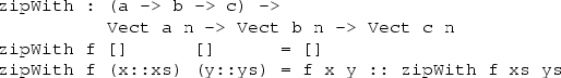
  • (b) Write a function to multiply two matrices.

3 Type Classes

We often want to define functions which work across several different data types. For example, we would like arithmetic operators to work on Int, Integer and Float at the very least. We would like == to work on the majority of data types. We would like to be able to display different types in a uniform way.

To achieve this, we use a feature which has proved to be effective in Haskell, namely type classes. To define a type class, we provide a collection of overloaded operations which describe the interface for instances of that class. A simple example is the Show type class, which is defined in the prelude and provides an interface for converting values to Strings:

This generates a function of the following type (which we call a method of the Show class):

We can read this as “under the constraint that a is an instance of Show, take an a as input and return a String.” An instance of a class is defined with an instance declaration, which provides implementations of the function for a specific type. For example, the Show instance for Nat could be defined as:

Like Haskell, by default only one instance of a class can be given for a type—instances may not overlap⁴. Also, type classes and instances may themselves have constraints, for example:

3.1 Monads and do-Notation

In general, type classes can have any number (greater than 0) of parameters, and the parameters can have any type. If the type of the parameter is not Type, we need to give an explicit type declaration. For example:

The Monad class allows us to encapsulate binding and computation, and is the basis of do-notation introduced in Sect. 2.6. Inside a do block, the following syntactic transformations are applied:

• $\mathtt{x~<-~v;~e}$ becomes $\mathtt{v~>>=}$ $\mathtt{(}\backslash \mathtt{x~=>~e)}$

• v; e becomes $\mathtt{v~>>=}$ $\mathtt{(}\backslash \mathtt{\_~=>~e)}$

• let x = v; e becomes let x = v in e

IO is an instance of Monad, defined using primitive functions. We can also define an instance for Maybe, as follows:

Using this we can, for example, define a function which adds two Maybe Ints, using the monad to encapsulate the error handling:

This function will extract the values from x and y, if they are available, or return Nothing if they are not. Managing the Nothing cases is achieved by the >>= operator, hidden by the do notation.

3.2 Idiom Brackets

While do notation gives an alternative meaning to sequencing, idioms give an alternative meaning to application. The notation and larger example in this section is inspired by Conor McBride and Ross Paterson’s paper “Applicative Programming with Effects” [12].

First, let us revisit m_add above. All it is really doing is applying an operator to two values extracted from Maybe Ints. We could abstract out the application:

Using this, we can write an alternative m_add which uses this alternative notion of function application, with explicit calls to m_app:

Rather than having to insert m_app everywhere there is an application, we can use idiom brackets to do the job for us. To do this, we use the Applicative class, which captures the notion of application for a data type:

Maybe is made an instance of Applicative as follows, where $\mathtt{<\$>}$ is defined in the same way as m_app above:

Using idiom brackets we can use this instance as follows, where a function application [| f a1 ... an |] is translated into $\mathtt{pure~f~<\$>~a1~<\$>~...~<\$>~an}$:

An Error-Handling Interpreter. Idiom brackets are often useful when defining evaluators for embedded domain specific languages. McBride and Paterson describe such an evaluator [12], for a small language similar to the following:

Evaluation will take place relative to a context mapping variables (represented as Strings) to integer values, and can possibly fail. We define a data type Eval to wrap an evaluation function:

We begin by defining a function to retrieve values from the context during evaluation:

When defining an evaluator for the language, we will be applying functions in the context of an Eval, so it is natural to make Eval an instance of Applicative. Before Eval can be an instance of Applicative it is necessary to make Eval an instance of Functor:

Evaluating an expression can now make use of the idiomatic application to handle errors:

By defining appropriate Monad and Applicative instances, we can overload notions of binding and application for specific data types, which can give more flexibility when implementing EDSLs. $\ldots \ldots$

4 Views and the “with” Rule

4.1 Dependent Pattern Matching

Since types can depend on values, the form of some arguments can be determined by the value of others. For example, if we were to write down the implicit length arguments to (++), we’d see that the form of the length argument was determined by whether the vector was empty or not:

If n was a successor in the [] case, or zero in the :: case, the definition would not be well typed.

4.2 The with Rule — Matching Intermediate Values

Very often, we need to match on the result of an intermediate computation. Idris provides a construct for this, the with rule, inspired by views in Epigram [11], which takes account of the fact that matching on a value in a dependently typed language can affect what we know about the forms of other values —we can learn the form of one value by testing another. For example, a Nat is either even or odd. If it’s even it will be the sum of two equal Nats. Otherwise, it is the sum of two equal Nats plus one:

We say Parity is a view of Nat. It has a covering function which tests whether it is even or odd and constructs the predicate accordingly.

We will return to this function in Sect. 5.5 to complete the definition of parity. For now, we can use it to write a function which converts a natural number to a list of binary digits (least significant first) as follows, using the with rule:

The value of the result of parity k affects the form of k, because the result of parity k depends on k. So, as well as the patterns for the result of the intermediate computation (even and odd) right of the $\vert$, we also write how the results affect the other patterns left of the $\vert$. Note that there is a function in the patterns (+) and repeated occurrences of j — this is allowed because another argument has determined the form of these patterns.

4.3 Membership Predicates

We have already seen (in Sect. 2.4) the Elem x xs type, an element of which is a proof that x is an element of the list xs:

We have also seen how to construct proofs of this at compile time. However, data is not often available at compile-time — proofs of list membership may arise due to user data, which may be invalid and therefore needs to be checked. What we need, therefore, is a function which constructs such a predicate, taking into account possible failure. In order to do so, we need to be able to construct equality proofs.

Propositional Equality. Idris allows propositional equalities to be declared, allowing theorems about programs to be stated and proved. Equality is built in, but conceptually has the following definition:

Equalities can be proposed between any values of any types, but the only way to construct a proof of equality is if values actually are equal. For example:

Decidable Equality. The library provides a Dec type, with two constructors, Yes and No. Dec represents decidable propositions, either containing a proof that a type is inhabited, or a proof that it is not. Here, _|_ represents the empty type, which we will discuss further in Sect. 5.1:

We can think of this as an informative version of Bool — not only do we know the truth of a value, we also have an explanation for it. Using this, we can write a type class capturing types which can not only be compared for equality, but which also provide a proof of that equality:

Using DecEq, we can construct equality proofs where necessary at run-time. There are instances defined in the prelude for primitive types, as well as many of the types defined in the prelude such as Bool, Maybe a, List a, etc.

Now that we can construct equality proofs dynamically, we can implement the following function, which dynamically constructs a proof that x is contained in a list xs, if possible:

This function works first by checking whether the list is empty. If so, the value cannot be contained in the list, so it returns Nothing. Otherwise, it uses decEq to try to construct a proof that the element is at the head of the list. If it succeeds, dependent pattern matching on that proof means that x must be at the head of the list. Otherwise, it searches in the tail of the list.

Exercises

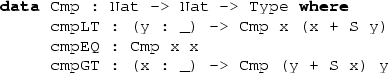
• 1. The following view describes a pair of numbers as a difference:

  

  • (a) Write the function cmp : (n : Nat) -> (m : Nat) -> Cmp n m which proves that every pair of numbers can be expressed in this way.

  • (b) Assume you have a vector xs : Vect a n, where n is unknown. How could you use cmp to construct a suitable input to vtake and vdrop from xs?

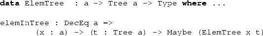
• 2. You are given the following definition of binary trees:

  

  Define a membership predicate ElemTree and a function elemInTree which calculates whether a value is in the tree, and a corresponding proof.

  

5 Theorem Proving

As we have seen in Sect. 4.3, Idris supports propositional equality:

We have used this to build membership proofs of Lists, but it is more generally applicable. In particular, we can reason about equality. The library function replace uses an equality proof to transform a predicate on one value into a predicate on another, equal, value:

The library function cong is a function defined in the library which states that equality respects function application:

Using the equality type, replace, cong and the properties of the type system, we can write proofs of theorems such as the following, which states that addition of natural numbers is commutative:

In this section, we will see how to develop such proofs.

5.1 The Empty Type

There is an empty type, $\bot$, which has no constructors. It is therefore impossible to construct an element of the empty type, at least without using a partially defined or general recursive function (which will be explained in more detail in Sect. 5.4). We can therefore use the empty type to prove that something is impossible, for example zero is never equal to a successor:

Here we use replace to transform a value of a type which can exist, the empty tuple, to a value of a type which can’t, by using a proof of something which can’t exist. Once we have an element of the empty type, we can prove anything. FalseElim is defined in the library, to assist with proofs by contradiction.

5.2 Simple Theorems

When type checking dependent types, the type itself gets normalised. So imagine we want to prove the following theorem about the reduction behaviour of plus:

We’ve written down the statement of the theorem as a type, in just the same way as we would write the type of a program. In fact there is no real distinction between proofs and programs. A proof, as far as we are concerned here, is merely a program with a precise enough type to guarantee a particular property of interest.

We won’t go into details here, but the Curry-Howard correspondence [10] explains this relationship. The proof itself is trivial, because plus Z n normalises to n by the definition of plus:

It is slightly harder if we try the arguments the other way, because plus is defined by recursion on its first argument. The proof also works by recursion on the first argument to plus, namely n.

We can do the same for the reduction behaviour of plus on successors:

Even for simple theorems like these, the proofs are a little tricky to construct directly. When things get even slightly more complicated, it becomes too much to think about to construct proofs in this ‘batch mode’. Idris therefore provides an interactive proof mode.

5.3 Interactive Theorem Proving

Instead of writing the proof in one go, we can use Idris’s interactive proof mode. To do this, we write the general structure of the proof, and use the interactive mode to complete the details. We’ll be constructing the proof by induction, so we write the cases for Z and S, with a recursive call in the S case giving the inductive hypothesis, and insert metavariables for the rest of the definition:

On running Idris, two global names are created, plusredZ_Z and plusredZ_S, with no definition. We can use the :m command at the prompt to find out which metavariables are still to be solved (or, more precisely, which functions exist but have no definitions), then the :t command to see their types and contexts:

The :p command enters interactive proof mode, which can be used to complete the missing definitions. This gives us a list of premises (above the line; there are none here) and the current goal (below the line; named {hole0} here). At the prompt we can enter tactics to direct the construction of the proof. In this case, we can normalise the goal with the compute tactic:

Now we have to prove that Z equals Z, which is easy to prove by refl. To apply a function, such as refl, we use refine which introduces subgoals for each of the function’s explicit arguments (refl has none):

Here, we could also have used the trivial tactic, which tries to refine by refl, and if that fails, tries to refine by each name in the local context. When a proof is complete, we use the qed tactic to add the proof to the global context, and remove the metavariable from the unsolved metavariables list. This also outputs a log of the proof:

The :addproof command, at the interactive prompt, will add the proof to the source file (effectively in an appendix). Let us now prove the other required lemma, plusredZ_S:

In this case, the goal is a function type, using k (the argument accessible by pattern matching) and ih — the local variable containing the result of the recursive call. We can introduce these as premises using the intro tactic twice (or intros, which introduces all arguments as premises). This gives:

Since plus is defined is defined by recursion on its first argument, the term plus (S k) 0 in the goal can be simplified using compute:

We know, from the type of ih, that k = plus k 0, so we would like to use this knowledge to replace plus k 0 in the goal with k. We can achieve this with the rewrite tactic:

The rewrite tactic takes an equality proof as an argument, and tries to rewrite the goal using that proof. Here, it results in an equality which is trivially provable:

Again, we can add this proof to the end of our source file using the :addproof command at the interactive prompt.

5.4 Totality Checking

If we really want to trust our proofs, it is important that they are defined by total functions. A total function is a function which is defined for all possible inputs and is guaranteed to terminate. Otherwise we could construct an element of the empty type, from which we could prove anything:

Internally, Idris checks every definition for totality, and we can check at the prompt with the :total command. We see that neither of the above definitions is total:

Note the use of the word “possibly” — a totality check can, of course, never be certain due to the undecidability of the halting problem. The check is, therefore, conservative. It is also possible (and indeed advisable, in the case of proofs) to mark functions as total so that it will be a compile time error for the totality check to fail:

Reassuringly, our proof in Sect. 5.1 that the zero and successor constructors are disjoint is total:

The totality check is, necessarily, conservative. To be recorded as total, a function f must:

• Cover all possible inputs.

• Be well-founded — i.e. by the time a sequence of (possibly mutually) recursive calls reaches f again, it must be possible to show that one of its arguments has decreased.

• Not use any data types which are not strictly positive.

• Not call any non-total functions.

Directives and Compiler Flags for Totality. By default, Idris allows all definitions, whether total or not. However, it is desirable for functions to be total as far as possible, as this provides a guarantee that they provide a result for all possible inputs, in finite time. It is possible to make total functions a requirement, either:

• By using the –total compiler flag.

• By adding a %default total directive to a source file. All definitions after this will be required to be total, unless explicitly flagged as partial.

All functions after a %default total declaration are required to be total. Correspondingly, after a %default partial declaration, the requirement is relaxed.

5.5 Provisional Definitions

Sometimes when programming with dependent types, the type required by the type checker and the type of the program we have written will be different (in that they do not have the same normal form), but nevertheless provably equal. For example, recall the parity function:

We would like to implement this as follows:

This simply states that zero is even, one is odd, and recursively, the parity of k+2 is the same as the parity of k. Explicitly marking the value of n in even and odd is necessary to help type inference. Unfortunately, the type checker rejects this:

The type checker is telling us that (j+1)+(j+1) and 2+j+j do not normalise to the same value. This is because plus is defined by recursion on its first argument, and in the second value, there is a successor symbol on the second argument, so this will not help with reduction. These values are obviously equal—how can we rewrite the program to fix this problem?

Provisional definitions help with this problem by allowing us to defer the proof details until a later point. There are two main motivations for supporting provisional definitions:

• When prototyping, it is useful to be able to test programs before finishing all the details of proofs. This is particularly useful if testing reveals that we would need to prove something which is untrue!

• When reading a program, it is often much clearer to defer the proof details so that they do not distract the reader from the underlying algorithm.

Provisional definitions are written in the same way as ordinary definitions, except that they introduce the right hand side with a ?= rather than =. We define parity as follows:

When written in this form, instead of reporting a type error, Idris will insert a metavariable standing for a theorem which will correct the type error. Idris tells us we have two proof obligations, with names generated from the module and function names:

The first of these has the following type and context:

The two arguments are j, the variable in scope from the pattern match, and value, which is the value we gave in the right hand side of the provisional definition. Our aim is to rewrite the type so that we can use this value. We can achieve this using the following theorem from the prelude:

After starting the theorem prover with :p parity_lemma_1 and applying intro twice, we have:

We need to use compute to unfold the definition of (+).

Then we apply the plusSuccRightSucc rewrite rule, symmetrically, to j and j, giving:

sym is a function, defined in the library, which reverses the order of the rewrite:

We can complete this proof using the trivial tactic, which finds value in the premises. The proof of the second lemma proceeds in exactly the same way.

We can now test the natToBin function from Sect. 4.2 at the prompt. The number 42 is 101010 in binary. The binary digits are reversed:

5.6 Suspension of Disbelief

Idris requires that proofs be complete before compiling programs (although evaluation at the prompt is possible without proof details). Sometimes, especially when prototyping, it is easier not to have to do this. It might even be beneficial to test programs before attempting to prove things about them — if testing finds an error, you know you should not waste your time proving something!

Therefore, Idris provides a built-in coercion function, which allows you to use a value of the incorrect types:

Obviously, this should be used with caution. It is useful when prototyping, and can also be appropriate when asserting properties of external code (perhaps in an external C library). The “proof” of views.parity_lemma_1 using this is:

The exact tactic allows us to provide an exact value for the proof. In this case, we assert that the value we gave was correct.

5.7 Example: Binary Numbers

Previously, we implemented conversion to binary numbers using the Parity view. Here, we show how to use the same view to implement a verified conversion to binary. We begin by indexing binary numbers over their Nat equivalent. This is a common pattern, linking a representation (in this case Binary) with a meaning (in this case Nat):

bO and bI take a binary number as an argument and effectively shift it one bit left, adding either a zero or one as the new least significant bit. The index, n + n or S (n + n) states the result that this left shift then add will have to the meaning of the number. This will result in a representation with the least significant bit at the front.

Now a function which converts a Nat to binary will state, in the type, that the resulting binary number is a faithful representation of the original Nat:

The Parity view makes the definition fairly simple — halving the number is effectively a right shift after all — although we need to use a provisional definition in the odd case:

The problem with the odd case is the same as in the definition of parity, and the proof proceeds in the same way:

To finish, we’ll implement a main program which reads an integer from the user and outputs it in binary.

For this to work, of course, we need a Show instance for Binary n:

Exercises

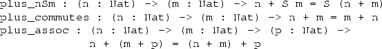
• 1. Implement the following functions, which verify some properties of natural number addition:

  

• 2. One way we have seen to define a reverse function for lists is as follows:

  

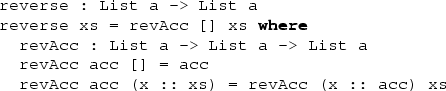
  Write the equivalent function for vectors,

  

  Hint: You can use the same structure as the definition for List, but you will need to think carefully about the type for revAcc, and may need to do some theorem proving.

6 EDSL Example 1: The Well-Typed Interpreter

In this section, we will use the features we have seen so far to write a larger example, an interpreter for a simple functional programming language, implemented as an Embedded Domain Specific Language. The object language (i.e., the language we are implementing) has variables, function application, binary operators and an if...then...else construct. We will use the type system from the host language (i.e. Idris) to ensure that any programs which can be represented are well-typed.

First, let us define the types in the language. We have integers, booleans, and functions, represented by Ty:

We can write a function to translate these representations to a concrete Idris type — remember that types are first class, so can be calculated just like any other value:

We will define a representation of our language in such a way that only well-typed programs can be represented. We index the representations of expressions by their type and the types of local variables (the context), which we’ll be using regularly as an implicit argument, so we define everything in a using block:

The full representation of expressions is given in Listing 3. They are indexed by the types of the local variables, and the type of the expression itself:

Since expressions are indexed by their type, we can read the typing rules of the language from the definitions of the constructors. Let us look at each constructor in turn.

We use a nameless representation for variables — they are de Bruijn indexed. Variables are represented by a proof of their membership in the context, HasType i G T, which is a proof that variable i in context G has type T. This is defined as follows:

We can treat stop as a proof that the most recently defined variable is well-typed, and pop n as a proof that, if the nth most recently defined variable is well-typed, so is the n+1th. In practice, this means we use stop to refer to the most recently defined variable, pop stop to refer to the next, and so on, via the Var constructor:

So, in an expression $\backslash$ x. $\backslash$ y. x y, the variable x would have a de Bruijn index of 1, represented as pop stop, and y 0, represented as stop. We find these by counting the number of lambdas between the definition and the use.

A value carries a concrete representation of an integer:

A lambda creates a function. In the scope of a function of type a -> t, there is a new local variable of type a, which is expressed by the context index:

Function application produces a value of type t given a function from a to t and a value of type a:

Given these constructors, the expression $\backslash$ x. $\backslash$ y. x y above would be represented as Lam (Lam (App (Var (pop stop)) (Var stop))).

We also allow arbitrary binary operators, where the type of the operator informs what the types of the arguments must be:

Finally, If expressions make a choice given a boolean. Each branch must have the same type, and we will evaluate the branches lazily so that only the branch which is taken need be evaluated:

When we evaluate an Expr, we’ll need to know the values in scope, as well as their types. Env is an environment, indexed over the types in scope. Since an environment is just another form of list, albeit with a strongly specified connection to the vector of local variable types, we use the usual :: and Nil constructors so that we can use the usual list syntax. Given a proof that a variable is defined in the context, we can then produce a value from the environment:

Given this, an interpreter (Listing 4) is a function which translates an Expr into a concrete Idris value with respect to a specific environment:

To translate a variable, we simply look it up in the environment:

To translate a value, we just return the concrete representation of the value:

Lambdas are more interesting. In this case, we construct a function which interprets the scope of the lambda with a new value in the environment. So, a function in the object language is translated to an Idris function:

For an application, we interpret the function and its argument and apply it directly. We know that interpreting f must produce a function, because of its type:

Operators and If expressions are, again, direct translations into the equivalent Idris constructs. For operators, we apply the function to its operands directly, and for If, we apply the Idris if...then...else construct directly.

We can make some simple test functions. Firstly, adding two inputs $\backslash \mathtt x.$ $\backslash \mathtt{y.~y~+~x}$ is written as follows:

More interestingly, we can write a factorial function (i.e. $\backslash$ x. if (x == 0) then 1 else (fact (x-1) * x)) which is written as follows:

To finish, we write a main program which interprets the factorial function on user input:

Here, cast is an overloaded function which converts a value from one type to another if possible. Here, it converts a string to an integer, giving 0 if the input is invalid. An example run of this program at the Idris interactive environment is shown in Listing 5.

Aside: cast. The prelude defines a type class Cast which allows conversion between types:

It is a multi-parameter type class, defining the source type and object type of the cast. It must be possible for the type checker to infer both parameters at the point where the cast is applied. There are casts defined between all of the primitive types, as far as they make sense.

7 Interactive Editing

By now, we have seen several examples of how Idris’ dependent type system can give extra confidence in a function’s correctness by giving a more precise description of its intended behaviour in its type. We have also seen an example of how the type system can help with EDSL development by allowing a programmer to describe the type system of an object language. However, precise types give us more than verification of programs — we can also exploit types to help write programs which are correct by construction.

The Idris REPL provides several commands for inspecting and modifying parts of programs, based on their types, such as case splitting on a pattern variable, inspecting the type of a metavariable, and even a basic proof search mechanism. In this section, we explain how these features can be exploited by a text editor, and specifically how to do so in Vim⁵. An interactive mode for Emacs⁶ is also available.

7.1 Editing at the REPL

The REPL provides a number of commands, which we will describe shortly, which generate new program fragments based on the currently loaded module. These take the general form

That is, each command acts on a specific source line, at a specific name, and outputs a new program fragment. Each command has an alternative form, which updates the source file in-place:

When the REPL is loaded, it also starts a background process which accepts and responds to REPL commands, using idris –client. For example, if we have a REPL running elsewhere, we can execute commands such as:

A text editor can take advantage of this, along with the editing commands, in order to provide interactive editing support.

7.2 Editing Commands

:addclause. The :addclause n f command (abbreviated :ac n f) creates a template definition for the function named f declared on line n.

For example, if the code beginning on line 94 contains$\ldots$

$\ldots$ then :ac 94 vzipWith will give:

The names are chosen according to hints which may be given by a programmer, and then made unique by the machine by adding a digit if necessary. Hints can be given as follows:

This declares that any names generated for types in the Vect family should be chosen in the order xs, ys, zs, ws.

:casesplit. The :casesplit n x command, abbreviated :cs n x, splits the pattern variable x on line n into the various pattern forms it may take, removing any cases which are impossible due to unification errors. For example, if the code beginning on line 94 is$\ldots$

$\ldots$ then :cs 96 xs will give:

That is, the pattern variable xs has been split into the two possible cases [] and x :: xs. Again, the names are chosen according to the same heuristic. If we update the file (using :cs!) then case split on ys on the same line, we get:

That is, the pattern variable ys has been split into one case [], Idris having noticed that the other possible case y :: ys would lead to a unification error.

:addmissing. The :addmissing n f command, abbreviated :am n f, adds the clauses which are required to make the function f on line n cover all inputs. For example, if the code beginning on line 94 is$\ldots$

$\ldots$ then :am 96 vzipWith gives:

That is, it notices that there are no cases for non-empty vectors, generates the required clauses, and eliminates the clauses which would lead to unification errors.

:proofsearch. The :proofsearch n f command, abbreviated :ps n f, attempts to find a value for the metavariable f on line n by proof search, trying values of local variables, recursive calls and constructors of the required family. Optionally, it can take a list of hints, which are functions it can try applying to solve the metavariable. For example, if the code beginning on line 94 is$\ldots$

$\ldots$ then :ps 96 vzipWith_rhs_1 will give

This works because it is searching for a Vect of length 0, of which the empty vector is the only possibility. Similarly, and perhaps surprisingly, there is only one possibility if we try to solve :ps 97 vzipWith_rhs_2:

This works because vzipWith has a precise enough type: The resulting vector has to be non-empty (::); the first element must have type c and the only way to get this is to apply f to x and y; finally, the tail of the vector can only be built recursively.

:makewith. The :makewith n f command, abbreviated :mw n f, adds a with to a pattern clause. For example, recall parity. If line 10 is$\ldots$

$\ldots$ then :mw 10 parity will give:

If we then fill in the placeholder _ with parity k and case split on with_pat using :cs 11 with_pat we get the following patterns:

Note that case splitting has normalised the patterns here (giving plus rather than +). In any case, we see that using interactive editing significantly simplifies the implementation of dependent pattern matching by showing a programmer exactly what the valid patterns are.

7.3 Interactive Editing in Vim

The editor mode for Vim provides syntax highlighting, indentation and interactive editing support using the commands described above. Interactive editing is achieved using the following editor commands, each of which update the buffer directly:

• $\backslash$ d adds a template definition for the name declared on the current line (using :addclause.)

• $\backslash$ c case splits the variable at the cursor (using :casesplit.)

• $\backslash$ m adds the missing cases for the name at the cursor (using :addmissing.)

• $\backslash$ w adds a with clause (using :makewith.)

• $\backslash$ o invokes a proof search to solve the metavariable under the cursor (using :proofsearch.)

• $\backslash$ p invokes a proof search with additional hints to solve the metavariable under the cursor (using :proofsearch.)

There are also commands to invoke the type checker and evaluator:

• $\backslash$ t displays the type of the (globally visible) name under the cursor. In the case of a metavariable, this displays the context and the expected type.

• $\backslash$ e prompts for an expression to evaluate.

• $\backslash$ r reloads and type checks the buffer.

Corresponding commands are also available in the Emacs mode. Support for other editors can be added in a relatively straighforward manner by using idris –client.

Exercises

Re-implement the following functions using interactive editing mode as far as possible:

When does :proofsearch succeed and when does it fail? How often does it provide the definition you would expect?

8 Support for EDSL Implementation

Idris supports the implementation of EDSLs in several ways. For example, as we have already seen, it is possible to extend do notation and idiom brackets. Another important way is to allow extension of the core syntax. In this section I describe further support for EDSL development. I introduce syntax rules and dsl notation [8], and describe how to make programs more concise with implicit conversions.

8.1 syntax Rules

We have seen if...then...else expressions, but these are not built in — instead, we define a function in the prelude, using laziness annotations to ensure that the branches are only evaluated if required$\ldots$

$\ldots$ and extend the core syntax with a syntax declaration:

The left hand side of a syntax declaration describes the syntax rule, and the right hand side describes its expansion. The syntax rule itself consists of:

• Keywords — here, if, then and else, which must be valid identifiers.

• Non-terminals — included in square brackets, [test], [t] and [e] here, which stand for arbitrary expressions. To avoid parsing ambiguities, these expressions cannot use syntax extensions at the top level (though they can be used in parentheses.)

• Names — included in braces, which stand for names which may be bound on the right hand side.

• Symbols — included in quotations marks, e.g. ":=". This can also be used to include reserved words in syntax rules, such as "let" or "in".

The limitations on the form of a syntax rule are that it must include at least one symbol or keyword, and there must be no repeated variables standing for non-terminals. Any expression can be used, but if there are two non-terminals in a row in a rule, only simple expressions may be used (that is, variables, constants, or bracketed expressions). Rules can use previously defined rules, but may not be recursive. The following syntax extensions would therefore be valid:

Syntax rules may also be used to introduce alternative binding forms. For example, a for loop binds a variable on each iteration:

Note that we have used the {x} form to state that x represents a bound variable, substituted on the right hand side. We have also put "in" in quotation marks since it is already a reserved word.

8.2 dsl Notation

The well-typed interpreter in Sect. 6 is a simple example of a common programming pattern with dependent types, namely: describe an object language and its type system with dependent types to guarantee that only well-typed programs can be represented, then program using that representation. Using this approach we can, for example, write programs for serialising binary data [2] or running concurrent processes safely [6].

Unfortunately, the form of object language programs makes it rather hard to program this way in practice. Recall the factorial program in Expr for example:

It is hard to expect EDSL users to program in this style! Therefore, Idris provides syntax overloading [8] to make it easier to program in such object languages:

A dsl block describes how each syntactic construct is represented in an object language. Here, in the expr language, any Idris lambda is translated to a Lam constructor; any variable is translated to the Var constructor, using pop and stop to construct the de Bruijn index (i.e., to count how many bindings since the variable itself was bound). It is also possible to overload let in this way. We can now write fact as follows:

In this new version, expr declares that the next expression will be overloaded. We can take this further, using idiom brackets, by declaring:

Note that there is no need for these to be part of an instance of Applicative, since idiom bracket notation translates directly to the names and pure, and ad-hoc type-directed overloading is allowed. We can now say:

With some more ad-hoc overloading and type class instances, and a new syntax rule, we can even go as far as:

8.3 Auto Implicit Arguments

We have already seen implicit arguments, which allows arguments to be omitted when they can be inferred by the type checker, e.g.

In other situations, it may be possible to infer arguments not by type checking but by searching the context for an appropriate value, or constructing a proof. For example, the following definition of head which requires a proof that the list is non-empty:

If the list is statically known to be non-empty, either because its value is known or because a proof already exists in the context, the proof can be constructed automatically. Auto implicit arguments allow this to happen silently. We define head as follows:

The auto annotation on the implicit argument means that Idris will attempt to fill in the implicit argument using the trivial tactic, which searches through the context for a proof, and tries to solve with refl if a proof is not found. Now when head is applied, the proof can be omitted. In the case that a proof is not found, it can be provided explicitly as normal:

More generally, we can fill in implicit arguments with a default value by annotating them with default. The definition above is equivalent to:

8.4 Implicit Conversions

Idris supports the creation of implicit conversions, which allow automatic conversion of values from one type to another when required to make a term type correct. This is intended to increase convenience and reduce verbosity. A contrived but simple example is the following:

In general, we cannot append an Int to a String, but the implicit conversion function intString can convert x to a String, so the definition of test is type correct. An implicit conversion is implemented just like any other function, but given the implicit modifier, and restricted to one explicit argument.

Only one implicit conversion will be applied at a time. That is, implicit conversions cannot be chained. Implicit conversions of simple types, as above, are however discouraged! More commonly, an implicit conversion would be used to reduce verbosity in an embedded domain specific language, or to hide details of a proof. We will see an example of this in the next section.

Exercises

• 1. Add a let binding construct to the Expr language from Sect. 6, and extend the interp function and dsl notation to handle it.

• 2. Define the following function, which updates the value in a variable:

  

• 3. Using update and let, you can extend Expr with imperative features. Add the following constructs:

  • (a) Sequencing actions

  • (b) Input and output operations

  • (c) for loops

  Note that you will need to change the type of interp so that it supports IO and returns an updated environment:

  

  For each of these features, how could you use syntax macros, dsl notation, or any other feature to improve the readability of programs in your language?

9 EDSL Example 2: A Resource Aware Interpreter

In a typical file management API, such as that in Haskell, we might find the following typed operations:

Unfortunately, it is easy to construct programs which are well-typed, but nevertheless fail at run-time, for example, if we read from a file opened for writing:

If we make the types more precise, parameterising open files by purpose, fprog is no longer well-typed, and will therefore be rejected at compile-time.

However, there is still a problem. The following program is well-typed, but fails at run-time — although the file has been closed, the handle h is still in scope:

Furthermore, we did not check whether the handle h was created successfully. Resource management problems such as this are common in systems programming — we need to deal with files, memory, network handles, etc., ensuring that operations are executed only when valid and errors are handled appropriately.

9.1 Resource Correctness as an EDSL

To tackle this problem, we can implement an EDSL which tracks the state of resources at any point during program execution in its type, and ensures that any resource protocol is correctly executed. We begin by categorising resource operations into creation, update and usage operations, by lifting them from IO. We illustrate this using Creator; Updater and Reader can be defined similarly.

The MkCreator constructor is left abstract, so that a programmer can lift an operation into Creator using ioc, but cannot run it directly. IO operations can be converted into resource operations, tagging them appropriately:

Here: open creates a resource, which may be either an error (represented by ()) or a file handle that has been opened for the appropriate purpose; close updates a resource from a File p to a () (i.e., it makes the resource unavailable); and read accesses a resource (i.e., it reads from it, and the resource remains available). They are implemented using the relevant (unsafe) IO functions from the Idris library. Resource operations are executed via a resource management EDSL, Res, with resource constructs (Listing 6), and control constructs (Listing 7).

As we did with Expr in Sect. 6, we index Res over the variables in scope (which represent resources), and the type of the expression. This means that firstly we can refer to resources by de Bruijn indices, and secondly we can express precisely how operations may be combined. Unlike Expr, however, we allow types of variables to be updated. Therefore, we index over the input set of resource states, and the output set:

We can read Res G G’ T as, “an expression of type T, with input resource states G and output resource states G’”. Expression types can be resources, values, or a choice type:

The distinction between resource types, R a, and value types, Val a, is that resource types arise from IO operations. A choice type corresponds to Either — we use Either rather than Maybe as this leaves open the possibility of returning informative error codes:

As with the interpreter in Sect. 6, we represent variables by proofs of context membership:

As well as a lookup function for retrieving values in an environment corresponding to a context, we also implement an update function:

The type of the Let construct explicitly shows that, in the scope of the Let expression, a new resource of type a is added to the set, having been made by a Creator operation. Furthermore, by the end of the scope, this resource must have been consumed (i.e. its type must have been updated to Val ()):

The Update construct applies an Updater operation, changing the type of a resource in the context. Here, using HasType to represent resource variables allows us to write the required type of the update operation simply as a -> Updater b, and put the operation first, rather than the variable.

The Use construct simply executes an operation without updating the context, provided that the operation is well-typed:

Finally, we provide a small set of control structures: Check, a branching construct that guarantees that resources are correctly defined in each branch; While, a loop construct that guarantees that there are no state changes during the loop; Lift, a lifting operator for IO functions, Return to inject pure values into a Res program, and (>>=) to support do-notation using ad-hoc name overloading. Note that we cannot make Res an instance of the Monad type class to support do-notation, since the type of >>= here captures updates in the resource set.

We use dsl-notation to overload the Idris syntax, in particular providing a let-binding to bind a resource and give it a human-readable name:

To further reduce notational overhead, we can make Lifting an IO operation implicit, using an implicit conversion as described in Sect. 8.4:

The interpreter for Res is written in continuation-passing style, where each operation passes on a result and an updated environment (containing resources):

The syntax rules provides convenient notations for declaring the type of a resource aware program, and for running a program in any context. For reference, the full interpreter is presented in Listing 8.

9.2 Example: File Management

We can use Res to implement a safe file-management protocol, where each file must be opened before use, opening a file must be checked, and files must be closed on exit. We define the following operations for opening, closing, reading a line⁷, and testing for the end of file.

Since these operations are now managed by the Res EDSL rather than directly as IO operations, we should ensure that the programmer cannot use the original IO operations. Names can be hidden using the %hide directive as follows:

Returning to our simple example from the beginning of this Section, we now write the file-reading program as follows:

This is well-typed because the file is opened for reading, and by the end of the scope, the file has been closed. Syntax overloading allows us to name the resource h rather than using a de Bruijn index or context membership proof.

10 An EDSL for Managing Side Effects

The resource aware EDSL presented in the previous section handles an instance of a more general problem, namely how to deal with side-effects and state in a pure functional language.

In this section, I describe how to implement effectful programs in Idris using an EDSL Effects for capturing algebraic effects [1], in such a way that they are easily composable, and translatable to a variety of underlying contexts using effect handlers. I will give a collection of example effects (State, Exceptions, File and Console I/O, random number generation and non-determinism) and their handlers, and some example programs which combine effects.

The Effects EDSL makes essential use of dependent types, firstly to verify that a specific effect is available to an effectful program using simple automated theorem proving, and secondly to track the state of a resource by updating its type during program execution. In this way, we can use the Effects DSL to verify implementations of resource usage protocols.

The framework consists of a DSL representation Eff for combining mutable effects and implementations of several predefined effects. We refer to the whole framework with the name Effects. Here, we describe how to use Effects; implementation details are described elsewhere [4].

The Effects library is included as part of the main Idris distribution, but is not imported by default. In order to use it, you must invoke Idris with the -p effects flag, and use the following in your programs:

10.1 Programming with Effects

An effectful program f has a type of the following form:

That is, the return type gives the effects that f supports (effs, of type List EFFECT), the effects available after running f (effs’) which may be calculated using the result of the operation result of type t.

A function which does not update its available effects has a type of the following form:

In fact, the notation { eff } is itself syntactic sugar, in order to make Eff types more readable. In full, the type of Eff is:

That is, it is indexed over the type of the computation, the list of input effects and a function which computes the output effects from the result. With syntax overloading, we can create syntactic sugar which allows us to write Eff types as described above:

Side effects are described using the EFFECT type; we will refer to these as concrete effects. For example:

States are parameterised by the type of the state being carried, and exceptions are parameterised by a type representing errors. File I/O allows a single file to be processed, with the type giving the current state of the file (i.e. closed, open for reading, or open for writing). Finally, STDIO and RND permit console I/O and random number generation respectively. For example, a program with some integer state, which performs console I/O and which could throw an exception carrying some error type Err would have the following type:

First Example: State. In general, an effectful program implemented in the Eff structure has the look and feel of a monadic program written with do-notation. To illustrate basic usage, let us implement a stateful function, which tags each node in a binary tree with a unique integer, depth first, left to right. We declare trees as follows:

To tag each node in the tree, we write an effectful program which, for each node, tags the left subtree, reads and updates the state, tags the right subtree, then returns a new node with its value tagged. The type expresses that the program requires an integer state:

The implementation traverses the tree, using get and put to manipulate state:

The Effects system ensures, statically, that any effectful functions which are called (get and put here) require no more effects than are available. The types of these functions are:

A program in Eff can call any other function in Eff provided that the calling function supports at least the effects required by the called function. In this case, it is valid for tag to call both get and put because all three functions support the STATE Int effect.

To run a program in Eff, it is evaluated in an appropriate computation context, using the run or runPure function. The computation context explains how each effectful operation, such as get and put here, are to be executed in that context. Using runPure, which runs an effectful program in the identity context, we can write a runTag function as follows, using put to initialise the state:

Effects and Resources. Each effect is associate with a resource, which is initialised before an effectful program can be run. For example, in the case of STATE Int the corresponding resource is the integer state itself. The types of runPure and run show this (slightly simplified here for illustrative purposes):

The env argument is implicit, and initialised automatically where possible using default values given by instances of the following type class:

Instances of Default are defined for all primitive types, and many library types such as List, Vect, Maybe, pairs, etc. However, where no default value exists for a resource type (for example, you may want a STATE type for which there is no Default instance) the resource environment can be given explicitly using one of the following functions:

To be well-typed, the environment must contain resources corresponding exactly to the effects in xs. For example, we could also have implemented runTag by initialising the state as follows:

As we will see, the particular choice of computation context can be important. Programs with exceptions, for example, can be run in the context of IO, Maybe or Either.

Labelled Effects. What if we have more than one state, especially more than one state of the same type? How would get and put know which state they should be referring to? For example, how could we extend the tree tagging example such that it additionally counts the number of leaves in the tree? One possibility would be to change the state so that it captured both of these values, e.g.:

Doing this, however, ties the two states together throughout (as well as not indicating which integer is which). It would be nice to be able to call effectful programs which guaranteed only to access one of the states, for example. In a larger application, this becomes particularly important.

The Effects library therefore allows effects in general to be labelled so that they can be referred to explicitly by a particular name. This allows multiple effects of the same type to be included. We can count leaves and update the tag separately, by labelling them as follows:

The ::: operator allows an arbitrary label to be given to an effect. This label can be any type—it is simply used to identify an effect uniquely. Here, we have used a symbol type. In general ’name introduces a new symbol, the only purpose of which is to disambiguate values⁸.

When an effect is labelled, its operations are also labelled using the :- operator. In this way, we can say explicitly which state we mean when using get and put. The tree tagging program which also counts leaves can be written as follows:

The update function here is a combination of get and put, applying a function to the current state.

Finally, our top level runTag function now returns a pair of the number of leaves, and the new tree. Resources for labelled effects are intialised using the := operator (reminiscent of assignment in an imperative language):

To summarise, we have:

• ::: to convert an effect to a labelled effect.

• :- to convert an effectful operation to a labelled effectful operation.

• := to initialise a resource for a labelled effect.

Or, more formally with their types (slightly simplified to account only for the situation where available effects are not updated):

Here, LRes is simply the resource type associated with a labelled effect. Note that labels are polymorphic in the label type lbl. Hence, a label can be anything—a string, an integer, a type, etc.

! -Notation. In many cases, using do-notation can make programs unnecessarily verbose, particularly in cases where the value bound is used once, immediately. The following program returns the length of the String stored in the state, for example:

This seems unnecessarily verbose, and it would be nice to program in a more direct style in these cases. Idris provides !-notation to help with this. The above program can be written instead as:

The notation !expr means that the expression expr should be evaluated and then implicitly bound. Conceptually, we can think of ! as being a prefix function with the following type:

Note, however, that it is not really a function, merely syntax! In practice, a subexpression !expr will lift expr as high as possible within its current scope, bind it to a fresh name x, and replace !expr with x. Expressions are lifted depth first, left to right. In practice, !-notation allows us to program in a more direct style, while still giving a notational clue as to which expressions are effectful.

For example, the expression$\ldots$

$\ldots$ is lifted to:

10.2 An Effectful Evaluator

Consider an evaluator for a simple expression language, supporting variables, integers, addition and random number generation, declared as follows:

In order to implement an evaluator for this language, we will need to carry a state, holding mappings from variables to values, and support exceptions (to handle variable lookup failure) and random numbers. The environment is simply a mapping from Strings representing variable names to Integers:

The evaluator invokes supported effects where needed. We use the following effectful functions:

The evaluator itself (Listing 9) is written as an instance of Eff, invoking the required effectful functions with the Effects framework checking that they are available.

In order to run the evaluator, we must provide initial values for the resources associated with each effect. Exceptions require the unit resource, random number generation requires an initial seed, and the state requires an initial environment. We use Maybe as the computation context to be able to handle exceptions:

Extending the evaluator with a new effect, such as STDIO is a matter of extending the list of available effects in its type. We could use this, for example, to print out the generated random numbers:

We can insert the STDIO effect anywhere in the list without difficulty. The only requirements are that its initial resource is in the corresponding position in the call to runInit, and that runInit instantiates a context which supports STDIO, such as IO:

10.3 Implementing Effects

In order to implement a new effect, we define a new type (of kind Effect) and explain how that effect is interpreted in some underlying context m. An Effect describes an effectful computation, parameterised by the type of the computation t, an input resource res, and an output resource res’ computed from the result of the operation.

We describe effects as algebraic data types. To run an effect, we require an interpretation in a computation context m. To achieve this, we make effects and contexts instances of a type class, Handler, which has a method handle explaining this interpretation:

Handlers are parameterised by the effect they handle, and the context in which they handle the effect. This allows several different context-dependent handlers to be written, e.g. exceptions could be handled differently in an IO setting than in a Maybe setting. When effects are combined, as in the evaluator example, all effects must be handled in the context in which the program is run.

An effect e t res res’ updates a resource type res to a resource type res’, returning a value t. The handler, therefore, implements this update in a context m which may support side effects. The handler is written in continuation passing style. This is for two reasons: firstly, it returns two values, a new resource and the result of the computation, which is more cleanly managed in a continuation than by returning a tuple; secondly, and more importantly, it gives the handler the flexibility to invoke the continuation any number of times (zero or more).

An Effect, which is the internal algebraic description of an effect, is promoted into a concrete EFFECT, which is expected by the Eff structure, with the MkEff constructor:

MkEff additionally records the resource state of an effect. In the remainder of this section, we describe how several effects can be implemented in this way: mutable state; console I/O; exceptions; files; random numbers, and non-determinism.

State. In general, effects are described algebraically in terms of the operations they support. In the case of State, the supported effects are reading the state (Get) and writing the state (Put).

The resource associated with a state corresponds to the state itself. So, the Get operation leaves this state intact (with a resource type a on entry and exit) but the Put operation may update this state (with a resource type a on entry and b on exit). That is, a Put may update the type of the stored value. Note that we are using the same syntactic sugar for updating the resource type as we used earlier for giving lists of effects. In full, State would be written as:

We can implement a handler for this effect, for all contexts m, as follows:

When running Get, the handler passes the current state to the continuation as both the return value (the second argument of the continuation k) and the new resource value (the first argument of the continuation). When running Put, the new state is passed to the continuation as the new resource value.

We then convert the algebraic effect State to a concrete effect usable in an Effects program using the STATE function, to which we provide the initial state type as follows:

As a convention, algebraic effects, of type Effect, have an initial upper case letter. Concrete effects, of type EFFECT, are correspondingly in all upper case.

Algebraic effects are promoted to Effects programs with concrete effects by using a coercion with an implicit, automatically constructed, proof argument:

How this function works and how the proof is calculated are beyond the scope of this tutorial. However, its purpose is to allow a programmer to use an algebraic effect in an Effects program without any explicit syntax. We can therefore define get and put as follows:

We may also find it useful to mutate the type of a state, considering that states may themselves have dependent types (we may, for example, add an element to a vector in a state). The Put constructor supports this, so we can implement putM to update the state’s type:

Finally, it may be useful to combine get and put in a single update:

Console I/O. Consider a simplified version of console I/O which supports reading and writing strings. There is no associated resource, although in an alternative implementation we may associate it with an abstract world state, or a pair of handles for stdin/stdout. Algebraically we describe console I/O as follows:

The obvious way to handle StdIO is via the IO monad:

Unlike the State effect, for which the handler worked in all contexts, this handler only applies to effectful programs run in an IO context. We can implement alternative handlers, and indeed there is no reason that effectful programs in StdIO must be evaluated in a monadic context. For example, we can define I/O stream functions:

A handler for StdIO in IOStream context generates a function from a list of strings (the input text) to a value and the output text. We can build a pure function which simulates real console I/O:

This requires an alternative means of running effectful programs, runWith, which takes an additional argument explaining how to inject the result of a computation into the appropriate computation context:

To illustrate this, we write a simple console I/O program:

Using mkStrFn, we can run this as a pure function which uses a list of strings as its input, and gives a list of strings as its output. We can evaluate this at the Idris prompt:

This suggests that alternative, pure, handlers for console I/O, or any I/O effect, can be used for unit testing and reasoning about I/O programs without executing any real I/O.

Exceptions. The exception effect supports only one operation, Raise. Exceptions are parameterised over an error type e, so Raise takes a single argument to represent the error. The associated resource is of unit type, and since raising an exception causes computation to abort, raising an exception can return a value of any type.

The semantics of Raise is to abort computation, therefore handlers of exception effects do not call the continuation k. In any case, this should be impossible since passing the result to the continuation would require the ability to invent a value in any arbitrary type b! The simplest handler runs in a Maybe context:

Exceptions can be handled in any context which supports some representation of failed computations. In an Either e context, for example, we can use Left to represent the error case:

Random Numbers. Random number generation can be implemented as an effect, with the resource tracking the seed from which the next number will be generated. The Random effect supports one operation, getRandom, which requires an Int resource and returns the next number:

Handling random number generation shows that it is a state effect in disguise, where the effect updates the seed. This is a simple linear congruential pseudo-random number generator:

Alternative handlers could use a different, possibly more secure approach. In any case, we can implement a function which returns a random number between a lower and upper bound as follows:

Non-determinism. Non-determinism can be implemented as an effect Selection, in which a Select operation chooses one value non-deterministically from a list of possible values:

We can handle this effect in a Maybe context, trying every choice in a list given to Select until the computation succeeds:

The handler for Maybe produces at most one result, effectively performing a depth first search of the values passed to Select. The handler runs the continuation for every element of the list until the result of running the continuation succeeds.

Alternatively, we can find every possible result by handling selection in a List context:

We can use the Selection effect to implement search problems by non-deterministically choosing from a list of candidate solutions. For example, a solution to the n-queens problem can be implemented as follows. First, we write a function which checks whether a point on a chess board attacks another if occupied by a queen:

Then, given a column and a list of queen positions, we find the rows on which a queen may safely be placed in that column:

Finally, we compute a solution by accumulating a set of queen positions, column by column, non-deterministically choosing a position for a queen in each column.

We can run this in Maybe context, to retrieve one solution, or in List context, to retrieve all solutions. In a Maybe context, for example, we can define:

Then to find the first solution, we run getQueens at the REPL:

10.4 Dependent Effects

In the programs we have seen so far, the available effects have remained constant. Sometimes, however, an operation can change the available effects. The simplest example occurs when we have a state with a dependent type—adding an element to a vector also changes its type, for example, since its length is explicit in the type. In this section, we will see how Effects supports this. Firstly, we will see how states with dependent types can be implemented. Secondly, we will see how the effects can depend on the result of an effectful operation. Finally, we will see how this can be used to implement a type-safe and resource-safe protocol for file management.

Dependent States. Suppose we have a function which reads input from the console, converts it to an integer, and adds it to a list which is stored in a STATE. It might look something like the following:

But what if, instead of a list of integers, we would like to store a Vect, maintaining the length in the type?

This will not type check! Although the vector has length n on entry to readInt, it has length S n on exit. The Effects DSL allows us to express this as follows:

The notation { xs ==> xs’ } Eff a in a type means that the operation begins with effects xs available, and ends with effects xs’ available. Since the type is updated, we have used putM to update the state.

Result-Dependent Effects. Often, whether a state is updated could depend on the success or otherwise of an operation. In the readInt example, we might wish to update the vector only if the input is a valid integer (i.e. all digits). As a first attempt, we could try the following, returning a Bool which indicates success:

Unfortunately, this will not type check because the vector does not get extended in both branches of the case!

Clearly, the size of the resulting vector depends on whether or not the value read from the user was valid. We can express this in the type:

The notation { xs ==> {res} xs’ } Eff a in a type means that the effects available are updated from xs to xs’, and the resulting effects xs’ may depend on the result of the operation res, of type a. Here, the resulting effects are computed from the result ok—if True, the vector is extended, otherwise it remains the same. We also use with_val to return a result:

We cannot use pure here, as before, since pure does not allow the returned value to update the effects list. The purpose of with_val is to update the effects before returning. As a shorthand, we can write

$\ldots$ instead of$\ldots$

$\ldots$ so our program is:

When using the function, we will naturally have to check its return value in order to know what the new set of effects is. For example, to read a set number of values into a vector, we could write the following:

The case analysis on the result of readInt means that we know in each branch whether reading the integer succeeded, and therefore how many values still need to be read into the vector. What this means in practice is that the type system has verified that a necessary dynamic check (i.e. whether reading a value succeeded) has indeed been done.

Aside: Only case will work here. We cannot use if/then/else because the then and else branches must have the same type. The case construct, however, abstracts over the value being inspected in the type of each branch.

File Management. A practical use for dependent effects is in specifying resource usage protocols and verifying that they are executed correctly. For example, file management follows a resource usage protocol with the following (informally specified) requirements:

• It is necessary to open a file for reading before reading it

• Opening may fail, so the programmer should check whether opening was successful

• A file which is open for reading must not be written to, and vice versa

• When finished, an open file handle should be closed

• When a file is closed, its handle should no longer be used

These requirements can be expressed formally in Effects, by creating a FILE_IO effect parameterised over a file handle state, which is either empty, open for reading, or open for writing. The FILE_IO effect’s definition is given in Listing 10. Note that this effect is mainly for illustrative purposes—typically we would also like to support random access files and better reporting of error conditions.

In particular, consider the type of open:

This returns a Bool which indicates whether opening the file was successful. The resulting state depends on whether the operation was successful; if so, we have a file handle open for the stated purpose, and if not, we have no file handle. By case analysis on the result, we continue the protocol accordingly.

Given a function readFile (Listing 11) which reads from an open file until reaching the end, we can write a program which opens a file, reads it, then displays the contents and closes it, as follows, correctly following the protocol:

The type of dumpFile, with FILE_IO () in its effect list, indicates that any use of the file resource will follow the protocol correctly (i.e. it both begins and ends with an empty resource). If we fail to follow the protocol correctly (perhaps by forgetting to close the file, failing to check that open succeeded, or opening the file for writing) then we will get a compile-time error. For example, changing open name Read to open name Write yields a compile-time error of the following form:

In other words: when reading a file, we need a file which is open for reading, but the effect list contains a FILE_IO effect carrying a file open for writing.

Exercise Consider the interpreter you implemented in the Sect. 8 exercises. How could you use Effects to improve this? For example:

• 1. What should be the type of interp?

• 2. Can you separate the imperative parts from the evaluation? What are the effects required by each?

11 Conclusion

In this tutorial, we have covered the fundamentals of dependently typed programming in Idris, and particularly those features which support embedded domain specific language implementation (EDSL). We have seen several examples of EDSLs in Idris:

• A well-typed interpreter for the simply typed $\lambda$-calculus, which shows how to implement an EDSL where the type-correctness of programs in the object language is verified by the host language’s type system.

• An interpreter for a resource-safe EDSL, capturing the state of resources such as file handles at particular points during program execution, ensuring, at compile time, that a program can only execute operations which are valid at those points.

• An EDSL for managing side-effecting programs, which generalises the resource-safe EDSL and allows several effects and resource to be managed simultaneously.

11.1 Further Reading

Further information about Idris programming, and programming with dependent types in general, can be obtained from various sources:

• The Idris web site (http://idris-lang.org/), which includes links to tutorials, some lectures and the mailing list. In particular, the Idris tutorial [5] describes the language in full, including many features not discussed here such as type providers [9], the foreign function interface, and compiling via Javascript.

• The IRC channel # idris, on chat.freenode.net.

• Examining the prelude and exploring the samples in the distribution.

• Various papers (e.g. [2, 3, 7, 8]), which describe implementation techniques and programming idioms.

References

Bauer, A., Pretnar, M.: Programming with Algebraic Effects and Handlers (2012). http://arxiv.org/abs/1203.1539
Brady, E.: Idris - systems programming meets full dependent types. In: Programming Languages Meets Program Verification (PLPV 2011), pp. 43–54 (2011)
Brady, E.: Idris, a general-purpose dependently typed programming language: design and implementation. J. Funct. Program. 23, 552–593 (2013)
Brady, E.: Programming and reasoning with algebraic effects and dependent types. In: ICFP 2013: Proceedings of the 18th ACM SIGPLAN International Conference on Functional Programming. ACM (2013)
Brady, E.: Programming in Idris : a tutorial (2013)
Brady, E., Hammond, K.: Correct-by-construction concurrency: using dependent types to verify implementations of effectful resource usage protocols. Fundamenta Informaticae 102(2), 145–176 (2010)
Brady, E., Hammond, K.: Scrapping your inefficient engine: using partial evaluation to improve domain-specific language implementation. In: ICFP 2010: Proceedings of the 15th ACM SIGPLAN International Conference on Functional Programming, pp. 297–308. ACM, New York (2010)
Brady, E., Hammond, K.: Resource-safe systems programming with embedded domain specific languages. In: Russo, C., Zhou, N.-F. (eds.) PADL 2012. LNCS, vol. 7149, pp. 242–257. Springer, Heidelberg (2012)
Christiansen, D.: Dependent type providers. In: WGP 2013: Proceedings of the 9th ACM SIGPLAN Workshop on Generic Programming. ACM (2013)
Howard, W.A.: The formulae-as-types notion of construction. In: Seldin, J.P., Hindley, J.R. (eds.) To H.B.Curry: Essays on Combinatory Logic, Lambda Calculus and Formalism. Academic Press, New York (1980). A reprint of an unpublished manuscript from 1969
McBride, C., McKinna, J.: The view from the left. J. Funct. Program. 14(1), 69–111 (2004)
McBride, C., Paterson, R.: Applicative programming with effects. J. Funct. Program. 18, 1–13 (2008)
Peyton Jones, S., et al.: Haskell 98 language and libraries - the revised report (2002). http://www.haskell.org/
Acknowledgements
I am grateful to the Scottish Informatics and Computer Science Alliance (SICSA) for funding this research. I would also like to thank the many contributors to the Idris system and libraries, as well as the reviewers for their helpful and constructive suggestions.
Author information
Authors and Affiliations
Corresponding author
Editor information
Editors and Affiliations
Rights and permissions
Copyright information
© 2015 Springer International Publishing Switzerland
About this chapter
Cite this chapter
Brady, E. (2015). The Idris Programming Language. In: Zsók, V., Horváth, Z., Csató, L. (eds) Central European Functional Programming School. CEFP 2013. Lecture Notes in Computer Science(), vol 8606. Springer, Cham. https://doi.org/10.1007/978-3-319-15940-9_4
Download citation
DOI: https://doi.org/10.1007/978-3-319-15940-9_4
Published:
Publisher Name: Springer, Cham
Print ISBN: 978-3-319-15939-3
Online ISBN: 978-3-319-15940-9
eBook Packages: Computer ScienceComputer Science (R0)