Simulation

Abstract

The previous chapter dealt with one of the tools for performance analysis—queueing theory. This chapter concentrates on another tool—simulation. In this chapter, we provide an overview of simulation: its historical background, importance, characteristics, and stages of development.

Science without religion is lame, religion without science is blind.

—Albert Einstein

These keywords were added by machine and not by the authors. This process is experimental and the keywords may be updated as the learning algorithm improves.

The previous chapter dealt with one of the tools for performance analysis—queueing theory. This chapter concentrates on another tool—simulation. In this chapter, we provide an overview of simulation: its historical background, importance, characteristics, and stages of development.

There is a lot of confusion among students as to what simulation is really about. Some confuse simulation with emulation or numerical modeling. While emulation is building a prototype (either hardware or software or combination of both) to mimic the real system, simulation is “the process of designing a mathematical or logical model of a real system and then conducting computer-based experiments with the model to describe, explain, and predict the behavior of the real system” [1]. In other words, simulation is modeling the real system, while emulation is an imitation of the system.

Simulation is designing a model that resembles a real system in certain important aspects.

It can be viewed as the act of performing experiments on a model of a given system. It is a cost-effective method of solving engineering problems. With computers, simulations have been used with great success in solving diverse scientific and engineering problems.

Simulation emerged as a numerical problem-solving approach during World War II when the so-called Monte Carlo methods were successfully used by John Von Neumann and Stanislaw Ulam of Los Alamos laboratory. The Monte Carlo methods were applied to problems related to atomic bomb. Simulation was introduced into university curricula in the 1960s during which books and periodicals on simulation began to appear. The system that is being modeled is deterministic in Monte Carlo simulation, and stochastic in case of simulation [2].

Computer systems can be modeled at several levels of detail [3]: circuit-level, gate-level, and system-level. At the circuit-level, we employ simulation to analyze the switching behavior of various components of the circuit such as resistors, capacitors, and transistors. In the gate-level simulation, the circuit components are aggregated into a single element so that the element is analyzed from a functional standpoint. At the system-level, the system is represented as a whole rather than as in segments as in gate-level simulation. System-level simulation involves analyzing the entire system from a performance standpoint. It is this kind of simulation that we shall be concerned with in this chapter.

5.1 Why Simulation?

A large number of factors influence the decision to use any particular scientific technique to solve a given problem. The appropriateness of the technique is one consideration, and economy is another. In this section, we consider the various advantages of using simulation as a modeling technique.

A system can be simplified to an extent that it can be solved analytically. Such an analytical solution is desirable because it leads to a closed form solution (such as in Chap. 4) where the relationship between the variables is explicit. However, such a simplified form of the system is obtained by many several assumptions so as to make the solution mathematically tractable. Most real-life systems are so complex that some simplifying assumptions are not justifiable, and we must resort to simulation. Simulation imitates the behavior of the system over time and provides data as if the real system were being observed.

Simulation as a modeling technique is attractive for the following reasons [4, 5]:

• (1) It is the next best thing to observing a real system in operation.

• (2) It enables the analysis of very complicated systems. A system can be so complex that its description by a mathematical model is beyond the capabilities of the analyst. “When all else fails” is a common slogan for many such simulations.

• (3) It is straightforward and easy to understand and apply. It does not rely heavily on mathematical abstractions which require an expert to understand and apply. It can be employed by many more individuals.

• (4) It is useful in experimenting with new or proposed design prior to implementation. Once constructed, it may be used to analyze the system under different conditions. Simulation can also be used in assessing and improving an existing system.

• (5) It is useful in verifying or reinforcing analytic solutions.

A major disadvantage of simulation is that it may be costly because it requires large expenditure of time in construction, running, and validation.

5.2 Characteristics of Simulation Models

As mentioned earlier, a model is a representation of a system. It can be a replica, a prototype, or a smaller-scale system [6]. For most analysis, it is not necessary to account for all different aspects of the system. A model simplifies the system to sufficiently detailed level to permit valid conclusions to be drawn about the system. A given system can be represented by several models depending on the objectives being pursued by the analyst. A wide variety of simulation models have been developed over the years for system analysis. To clarify the nature of these models, it is necessary to understand a number of characteristics.

5.2.1 Continuous/Discrete Models

This characteristic has to do with the model variables. A continuous model is one in which the state variables change continuously with time. The model is characterized by smooth changes in the system state. A discrete model is one in which state variables assume a discrete set of values. The model is characterized by discontinuous changes in the system state. The arrival process of messages in the queue of a LAN is discrete since the state variable (i.e. the number of waiting messages) changes only at the arrival or departure of a message.

5.2.2 Deterministic/Stochastic Models

This characteristic deals with the system response. A system is deterministic if its response is completely determined by its initial state and input. It is stochastic (or non-deterministic) if the system response may assume a range of values for given initial state and input. Thus only the statistical averages of the output measures of a stochastic model are true characteristics of the real system. The simulation of a LAN usually involves random interarrival times and random service times.

5.2.3 Time/Event Based Models

Since simulation is the dynamic portray of the states of a system over time, a simulation model must be driven by an automatic internal clock. In time-based simulation, the simulation clock advances one “tick” of Δt. Figure 5.1 shows the flowchart of a typical time-based simulation model.

Fig. 5.1

Typical time-based simulation model

Although time-based simulation is simple, it is inefficient because some action must take place at each clock “tick.” An event signifies a change in state of a system. In event-based simulation model, updating only takes place at the occurrence of events and the simulation clock is advanced by the amount of time since the last event. Thus no two events can be processed at any pass. The need of determining which event is next in event-based simulation makes its programming complex. One disadvantage of this type of simulation is that the speed at which the simulation proceeds is not directly related to real time; correspondence to real time operation is lost. Figure 5.2 is the flow chart of a typical event-based simulation.

Fig. 5.2

Typical event-based simulation model

The concepts of event, process, and activity are important in building a system model. As mentioned earlier, an event is an instantaneous occurrence that may change the state of the system. It may occur at an isolated point in time at which decisions are made to start or end an activity.

A process is a time-ordered sequence of events. An activity represents a duration of time. The relationship of the three concepts is depicted in Fig. 5.3 for a process that comprises of five events and two activities. The concepts lead to three types of discrete simulation modeling [7]: event scheduling, activity scanning, and process interaction approaches.

Fig. 5.3

Relationship of events, activities, and processes

Fig. 5.4

Stages in model development

5.2.4 Hardware/Software Models

Digital modeling may involve either hardware or software simulation. Hardware simulation involves using a special purpose equipment, and detailed programming is reduced to a minimum. This equipment is sometimes called a simulator. In software simulation, the operation of the system is modeled using a computer program. The program describes certain aspects of the system that are of interest.

In this chapter, we are mainly concerned with software models that are discrete, stochastic, and event-based.

5.3 Stages of Model Development

Once it has been decided that software simulation is the appropriate methodology to solve a particular problem, there are certain steps a model builder must take. These steps parallel six stages involved in model development. (Note that the model is the computer program.) In programming terminology, these stages are [5, 9, 10]: (1) Model building, (2) program synthesis, (3) model verification, (4) model validation, (5) model analysis, and (6) documentation. The relationship of the stages is portrayed in Fig. 5.5, where the numbers refer to the stages.

Fig. 5.5

Common flowchart symbols

• 1. Model Building: This initial stage usually involves a thorough, detailed study of the system to decompose it into manageable levels of detail. The modeler often simplifies components or even omit some if their effects do not warrant their inclusion. The task of the modeler is to produce a simplified yet valid abstraction of the system. This involves a careful study of the system of interest. The study should reveal interactions, dependence, and rules governing the components of the system. It should also reveal the estimation of the system variables and parameters. The modeler may use flowcharts to define or identify subsystems and their interactions. Since flowcharting is a helpful tool in describing a problem and planning a program, commonly used symbols are shown in Fig. 5.5. These symbols are part of the flowcharting symbols formalized by the American National Standards Institute (ANSI). The modeler should feel free to adapt the symbols to his own style.

• 2. Program Synthesis: After a clear understanding of the simplified system and the interaction between components is gained, all the pieces are synthesized into a coherent description, which results in a computer program. The modeler must decide whether to implement the model in a general-purpose language such as FORTRAN or C++ or use a special-purpose simulation language such GASP, GPSS, SLAM, SIMULA, SIMSCRIPT, NS2 or OPNET. A special-purpose simulation language usually require lesser amount of development time, but executes slower than a general-purpose language. However, general-purpose languages so speed up programming and verification stages that they are becoming more and more popular in model development [5]. The selection of the type of computer and language to be used depends on resources available to the programmer.

• 3. Model Verification: This involves a logical proof of the correction of the program as a model. It entails debugging the simulation program and ensuring that the input parameters and logical structure of the model are correctly represented in the code. Although the programmer may know precisely what the program is intended to accomplish, the program may be doing something else.

• 4. Model Validation: This stage is the most crucial. Since models are simplified abstractions, the validity is important. A model is validated by proving that the model is a correct representation of the real system. A verified program can represent an invalid model. This stage ensures that the computer model matches the real system by comparing the two. This is easy when the real system exists. It becomes difficult when the real system does not exist. In this case, a simulator can be used to predict the behavior of the real system. Validation may entail using a statistical proof of correctness of the model. Whichever validation approach is used, validation must be performed before the model can be used. Validation may uncover further bugs and even necessitate reformulation of the model.

• 5. Model Analysis: Once the model has been validated, it can be applied to solve the problem at hand. This stage is the reason for constructing the model in the first place. It involves applying alternate input parameters to the program and observing their effects of the output parameters. The analysis provides estimate measures of performance of the system.

• 6. Documentation: The results of the analysis must be clearly and concisely documented for future references by the modeler or others. An inadequately documented program is usually useless to everyone including the modeler himself. Thus the importance of this step cannot be overemphasized.

5.4 Generation of Random Numbers

Fundamental to simulations is the need of having available sequences of numbers which appear to be drawn at random from a particular probability law. The method by which random numbers are generated is often called the random number generator [8, 10–12]. A simple way of generating random numbers is by casting a dice with six faces numbered 1 to 6. Another simple way is to use the roulette wheel (similar to the “wheel of fortune”). These simple ways, however, will not generate enough numbers to make them truly random.

The almost universally used method of generating random numbers is to select a function G(Z) that maps integers into random numbers. Select some guessed value Z₀, and generate the next random number as Z _n + 1 = G(Z _n ). The commonest function G(Z) takes the form

$$ \mathrm{G}\left(\mathrm{Z}\right)=\left(\mathrm{aZ}+\mathrm{c}\right)\ \mod\ \mathrm{m} $$

(5.1)

where

$$ {Z}_0=\mathrm{a}\ \mathrm{starting}\ \mathrm{value}\ \mathrm{or}\ \mathrm{a}\ \mathrm{seed}\kern0.5em \left({Z}_0\ge 0\right) $$

(5.2)

a = multiplier(a ≥ 0),

c = increment (c ≥ 0),

m = the modulus

The modulus m is usually 2^t for t-digit binary integers. For a 31-bit computer machine, for example, m may be 2^31 − 1. Here Z₀, a, and c are integers in the same range as m > a, m > c, m > Z₀.

The desired sequence of random numbers Z_n is obtained from

$$ {Z}_{n+1}=\left(a{Z}_n+c\right)\ \mod\ m $$

(5.3)

This is called a linear congruential sequence. For example, if Z₀ = a = c = 7 and m = 10, the sequence is

$$ 7,6,9,0,7,6,9,0,\dots $$

(5.4)

In practice, we are usually interested in generating random numbers U from the uniform distribution in the interval (0,1).

$$ U=\frac{Z_{n+1}}{m} $$

(5.5)

U can only assume values from the set {0, 1/m, 2/m, …, (m − 1)/m}. A set of uniformly distributed random numbers can be generated using the following procedure:

• (a) Select an odd number as a seed value Z₀.

• (b) Select the multiplier a = 8r ± 3, where r is any positive integer and a is close to 2^t/2. If t = 31, a = 2¹⁵ + 3 is a good choice.

• (c) Compute Z_n + 1 using either the multiplicative generator

  $$ {Z}_{n+1}=a{Z}_n\kern0.5em \mod\ m $$

  (5.6)

  or the mixed generator

  $$ {Z}_{n+1}=\left(a{Z}_n+c\right)\kern0.5em \mod\ m $$

  (5.7)

• (d) Compute U = Z_n + 1/m.

  U is uniformly distributed in the interval (0,1). For generating random numbers X uniformly distributed over the interval (A,B), we use

  $$ \mathrm{X}=\mathrm{A}+\left(\mathrm{B}-\mathrm{A}\right)\mathrm{U} $$

  (5.8)

Random numbers based on the above mathematical relations and computer-produced are not truly random. In fact, given the seed of the sequence, all numbers U of the sequence are completely predictable or deterministic. Some authors emphasize this point by calling such computer-generated sequences pseudorandom numbers.

Example 5.1

(a) Using linear congruential scheme, generate ten pseudorandom numbers with a = 573, c = 19, m = 10³, and seed value Z₀ = 89. Use these numbers to generate uniformly distributed random numbers 0 < U < 1. (b) Repeat the generation with c = 0.

Solution

• (a) This is a multiplicative generator. Substituting a = 573, c = 19, m = 1,000, and Z₀ = 89 in Eq. (5.3) leads to

  • Z₁ = 573 × 89 + 19 (mod 1,000) = 16

  • Z₂ = 573 × 16 + 19 (mod 1,000) = 187

  • Z₃ = 573 × 187 + 19 (mod 1,000) = 170

  • Z₄ = 573 × 170 + 19 (mod 1,000) = 429

  • Z₅ = 573 × 429 + 19 (mod 1,000) = 836

  • Z₆ = 573 × 836 + 19 (mod 1,000) = 47

  • Z₇ = 573 × 47 + 19 (mod 1,000) = 950

  • Z₈ = 573 × 950 + 19 (mod 1,000) = 369

  • Z₉ = 573 × 369 + 19 (mod 1,000) = 456

  • Z₁₀ = 573 × 456 + 19 (mod 1,000) = 307

  Dividing each number by m = 1,000 gives U as

  • 0.016, 0.187, 0.170, …,0.307

• (b) For c = 0, we have the mixed generator. Thus, we obtain

  • Z₁ = 573 × 89 (mod 1,000) = 997

  • Z₂ = 573 × 997 (mod 1,000) = 281

  • Z₃ = 573 × 281 (mod 1,000) = 13

  • Z₄ = 573 × 13 (mod 1,000) = 449

  • Z₅ = 573 × 449 (mod 1,000) = 277

  • Z₆ = 573 × 277 (mod 1,000) = 721

  • Z₇ = 573 × 721 (mod 1,000) = 133

  • Z₈ = 573 × 133 (mod 1,000) = 209

  • Z₉ = 573 × 209 (mod 1,000) = 757

  • Z₁₀ = 573 × 757 (mod 1,000) = 761

  with the corresponding U as

  • 0.997, 0.281, 0.013,…,0.761

5.5 Generation of Random Variables

It is often required in a simulation to generate random variable X from a given probability distribution F(x). The most commonly used techniques are the inverse transformation method and the rejection method [10, 13].

The inverse transformation method basically entails inverting the cumulative probability function F(x) = P[X ≤ x] associated with the random variable X. To generate a random variable X with cumulative probability distribution F(x), we set U = F(x) and obtain

$$ \mathrm{X}={\mathrm{F}}^{-1}\left(\mathrm{U}\right) $$

(5.9)

where X has the distribution function F(x).

If, for example, X is a random variable that is exponentially distributed with mean μ, then

$$ F(x)=1-{e}^{-x/\mu },\begin{array}{cc}\hfill \hfill & \hfill 0<x<\infty \hfill \end{array} $$

(5.10)

Solving for X in U = F(X) gives

$$ X=-\mu \ln \left(1-U\right) $$

(5.11)

Since (1 − U) is itself a random number in the interval (0,1), we can write

$$ X=-\mu \ln U $$

(5.12)

A number of distributions which can be generated using the inverse method are listed in Table 5.1.

Table 5.1 Applications of the inverse-transform method [14]

The rejection method can be applied to the probability distribution of any bounded variable. To apply the method, we let the probability density function of the random variable f(x) = 0 for a > x > b, and let f(x) be bounded by M (i.e. f(x) ≤ M) as shown in Fig. 5.6.

Fig. 5.6

The rejection method of generating a random variate from f(x)

We generate random variate by taking the following steps:

• (1) Generate two random numbers (U₁, U₂) in the interval (0,1).

• (2) Compute two random numbers with uniform distributions in (a,b) and (0,M) respectively, i.e.

  • X = a + (b − a) U₁ (scale the variable on the x-axis)

  • Y = U₂ M (scale the variable on the y-axis).

• (3) If Y ≤ f(X), accept X as the next random variate, otherwise reject X and return to Step 1.

Thus in the rejection technique all points falling above f(x) are rejected while those points falling on or below f(x) are utilized to generate X through X = a + (b − a)U₁.

The C codes for generating uniform and exponential variates using Eqs. (5.8) and (5.12) are shown in Fig. 5.7. RAND_MAX is defined in stdlb.h and defines the maximum random number generated by the rand() function. Also, EX represents the mean value of the exponential variates.

Fig. 5.7

Subroutines for generating random: (a) uniform, (b) exponential variates

Other random variables are generated as follows [14]:

• Bernoulli variates: Generate U. If U ≤ p, return 0. Otherwise, return 1.

• Erlang variates: Generate U in m places and then

  $$ \mathrm{Erlang}\left(a,m\right)\sim -a \ln \left({\displaystyle \prod_{k=1}^m{U}_k}\right) $$

• Geometric variates: Generate U and compute

  $$ G(p)=\left[\frac{ \ln U}{ \ln \left(1-p\right)}\right] $$

  where [.] denotes rounding up to the next larger integer.

• Gaussian (or normal) variates: Generate twelve U, obtain $Z={\displaystyle \sum_{k=1}^{12}{U}_k-6}$ and set X = σZ + μ

5.6 Simulation of Queueing Systems

For illustration purposes, we now apply the ideas in the previous sections specifically to M/M/1 and M/M/n queueing systems. Since this section is the heart of this chapter, we provide a lot of details to make the section as interesting, self-explanatory, and self-contained as possible.

5.6.1 Simulation of M/M/1 Queue

As shown in Fig. 5.8, the M/M/1 queue consists of a server which provides service for the customers who arrive at the system, receive service, and depart. It is a single-server queueing system with exponential interarrival times and exponential service times and first-in-first-out queue discipline. If a customer arrives when the server is busy, it joins the queue (the waiting line).

Fig. 5.8

M/M/1 queue

There are two types of events: customer arrivals (A) and departure events (D). The following quantities are needed in representing the model [15, 16]:

• AT = arrival time

• DT = departure time

• BS = Busy server (a Boolean variable)

• QL = queue length

• RHO = traffic intensity

• ART = mean arrival time

• SERT = mean service time

• CLK = simulation global clock

• CITs = customer interarrival times (random)

• CSTs = customer service times (random)

• TWT = total waiting time

• NMS = total no. of messages (or customers) served

The global clock CLK always has the simulated current time. It is advanced by AT, which is updated randomly. The total waiting time TWT is the accumulation of the times spent by all customers in the queue.

The simulator works as shown in the flowchart in Fig. 5.9a and explained as follows. As the first step, we initialize all variables.

Fig. 5.9

(a) Flowchart for the simulation of M/M/1 queue, (b) flowchart of the arrival event, (c) flowchart for the departure event

• CLK = 0 (simulation clock)

• QL = 0

• TWT = 0

• NMS = 0

• AT = 0

• BS = false

• DT = bigtime, say 10²⁵

• other variables = 0 or specify

The “bigtime” is selected such that it is greater than any value of CLK in the simulation.

As the second step, we determine the next event by checking whether AT > DT. By default the first event to occur is arrival of the first customer, as illustrated in Fig. 5.10. Whether the second or subsequent event is arrival or departure depends on whether AT < DT because AT and DT are generally random.

Fig. 5.10

The first few events in simulation

As the third step, update statistics depending on whether the event is arrival or departure. The occurrence of either will affect QL or BS. Since this step is crucial, the step is illustrated in Fig. 5.9b, c for arrival and department events respectively. For an arrival event, update statistics by updating the total waiting time and scheduling the next arrival event. If server is busy, increment queue size. If server is idle, make server busy and schedule departure/service event. For departure event, update the total waiting time, system clock, and increment the number of customers served. If queue is empty, disable departure event. As shown in Fig. 5.9c, the departure event is disabled by setting DT = bigtime. This will ensure that a customer does not exit the system before being served. If queue is not empty, make server busy, decrement queue size, and schedule next departure event.

As the fourth step, determine whether simulation should be stopped by checking when CLK ≤ TMAX (or when a large number of customers have been served, i.e. NMS ≤ NMAX). And as the last step, compute the mean/average values, i.e.

$$ \mathrm{Average}\kern0.5em \mathrm{queue}\kern0.5em \mathrm{length}=\kern0.5em \frac{\mathrm{TWT}}{\mathrm{CLK}} $$

(5.13)

$$ \mathrm{Average}\ \mathrm{waiting}\ \mathrm{time}\kern0.5em =\kern0.5em \frac{\mathrm{TWT}}{\mathrm{NMS}} $$

(5.14)

5.6.2 Simulation of M/M/n Queue

Figure 5.11 shows a M/M/n queue, in which n servers are attached to a single queue. Customers arrive following a Poisson counting process (i.e., exponential interarrival times). Each server serves the customers with exponentially distributed service times. Here, we assume that the mean service time is the same for all of the servers. If all the servers are busy, a new customer joins the queue. Otherwise, it will be served by one of the free servers. After serving a customer, the server can serve the customer waiting ahead of queue, if any.

Fig. 5.11

M/M/n queue

With a careful observation of the way that the customers are served, we can extend the C program for M/M/1 queue to take care of the more general, M/M/n queue. The following quantities should be defined as arrays instead of scalar quantities:

• DT[j]—departure time from the jth server, j = 1,2,…, n

• BS[j]—busy server jth, j = 1,2,…, n

We also define a variable named SERVER which is associated with the current event. The other quantities remain unchanged from the M/M/1 model. Figure 5.12a illustrates the flowchart of simulator for M/M/n queue.

Fig. 5.12

(a) Flowchart for the simulation of M/M/n queue, (b) flowchart of the arrival event, (c) flowchart for the departure event

As the first step, we initialize all variables at the start of the program just like for the M/M/1 queue (Fig. 5.9). The only difference here is with the two arrays for BS and DT.

• DT[j] = bigtime, j = 1,2, …, n

• BS[j] = false, j = 1,2,…, n

As the second step, we determine the next event by checking whether AT < DT [j] for all j = 1,2,…,n. If so, the program proceeds with the arrival event in the third step. Otherwise it finds the SERVER associated with the closest departure event.

As the third step, the program performs either the arrival or departure routine (Fig. 5.12b, c), and updates the statistics accordingly. For an arrival event, the program updates TWT and CLK and then checks to see if a server is free. If all the servers are busy, the queue is incremented by one. If some servers are free, the first available one is made busy and scheduled for a departure event. For departure event, only the server engaged in this event becomes free. If there is no customer in queue, this server remains idle and its departure event is assigned “bigtime.” When the queue is not empty, the server will be busy again and the next departure event will be scheduled.

Example 5.2

(a) Write a computer program to simulate an M/M/1 queue assuming that the arrival rate has a mean value of 1,000 bps and that the traffic intensity ρ = 0.1, 0.2,…, 0.9. Calculate and plot the average queue length and the average waiting time in the queue for various values of ρ. Compare your results with the exact analytical formulas. (b) Repeat part (a) for an M/D/1 queue.

Solution

• (a) Based on the flowchart given in Fig. 5.9 and the variables introduced above, we develop a program in C to implement the simulator for M/M/1 queue. In this example each single bit represents a customer, and the customers arrive 1,000 per second on average. The simulator runs according to the flowchart for each value of ρ = 0.1, 0.2, …,0.9. For each ρ, the simulator computes the output variables after enough number of customers (say 10,000) are served. The arrival rate is λ = 1,000 bps, and the mean interarrival time (1/λ) is 1 ms. For each ρ, the mean departure rate is μ = λ/ρ and the corresponding mean service time is 1/μ. In Fig. 5.13, the average waiting time and the average queue length for M/M/1 queue are shown. The results are given for both the simulation and analytical solution. The analytical formulas for M/M/1 queue are found in Chap. 4:

  Fig. 5.13

  

  (a) Average waiting time for M/M/1 queue; (b) Average queue length for M/M/1 queue

  $$ E(W)=\frac{\rho }{\mu \left(1-\rho \right)} $$

  (5.15)
  $$ E\left({N}_q\right)=\frac{\rho^2}{1-\rho } $$

  (5.16)

  where E(W) and E(N_q) are the average waiting time and queue length respectively.

• (b) For M/D/1 queue, the service times are deterministic or constant. The only change in the flowchart of Fig. 5.9 is replacing the statement

  • CST = −SERT*LOG(X)

  with CST = SERT. The analytical formulas for an M/D/1 queue are found in Chap. 4, namely:

  $$ E(W)=\frac{\rho }{2\mu \left(1-\rho \right)} $$

  (5.17)
  $$ E\left({N}_q\right)=\frac{\rho^2}{2\left(1-\rho \right)} $$

  (5.18)

  Figure 5.14 show the results for M/D/1 queue. We notice that both the average waiting time and queue length are half of their respective values for M/M/1 queue which is confirmed by simulation.

  Fig. 5.14

  

  (a) Average waiting time for M/D/1 queue; (b) Average queue length for M/D/1 queue

Example 5.3

Develop a computer program to simulate an M/M/n queue assuming that the arrival rate has a mean value of 1,000 bps and that traffic intensity ρ = 0.1, 0.2, …. Calculate and plot the average waiting time and the average queue length in the queue for n = 2 and n = 5 servers. Compare the results with those of M/M/1 queue.

Solution

We use the flowcharts in Fig. 5.12 to modify the program of the last example. Since n servers are serving the customers, the value of ρ can be up to n, without the queue being congested by high number of customer waiting. The analytical formulas for the average waiting time E(W) and queue length E(N_q) respectively are given by:

$$ E(W)=\frac{\rho^n\left(\rho /n\right)}{n!{\left(1-\rho /n\right)}^2}{p}_0 $$

(5.19)

$$ E\left({N}_q\right)=\lambda E(W) $$

(5.20)

where n is the number of servers and

$$ {p}_0={\left[{\displaystyle \sum_{k=0}^{n-1}\frac{\rho^k}{k!}+\frac{\rho^n}{n!}\frac{1}{\left(1-\rho /n\right)}}\right]}^{-1} $$

(5.21)

The average waiting time and the queue length are given in Fig. 5.15a, b. We observe good agreement between analytical and simulation results. We can also see that for a particular value of ρ, both the waiting time and queue length are smaller for the larger number of servers.

Fig. 5.15

(a) Average waiting time for M/M/n queue, n = 1, 2, 5. (b) Average queue length for M/M/n queue, n = 1, 2, 5

5.7 Estimation of Errors

Simulation procedures give solutions which are averages over a number of tests. For this reason, it is important to realize that the sample statistics obtained from simulation experiments will vary from one experiment to another. In fact, the sample statistics themselves are random variables and, as such, have associated probability distributions, means, variances, and standard deviation. Thus the simulation results contain fluctuations about a mean value and it is impossible to ascribe a 100 % confidence in the results. To evaluate the statistical uncertainty or error in a simulation experiment, we must resort to various statistical techniques associated with random variables and utilize the central limit theorem.

Suppose that X is a random variable. You recall that we define the expected or mean value of X as

$$ \mu ={\displaystyle \underset{-\infty }{\overset{\infty }{\int }} xf(x) dx} $$

(5.22)

where f(x) is the probability density distribution of X. If we draw random and independent samples, x ₁, x ₂, ⋯, x _N from f(x), our estimate of x would take the form of the mean of N samples, namely,

$$ \tilde{\mu}=\frac{1}{N}{\displaystyle \sum_{n=1}^N{x}_n} $$

(5.23)

Whereas μ is the true mean value of X, $\tilde{\mu}$ is the unbiased estimator of μ—an unbiased estimator being one with the correct expectation value. Although expected value $\tilde{\mu}$ is close to μ but $\tilde{\mu}\ne \mu$. The standard deviation, defined as

$$ \sigma (x)={\left[E\left({X}^2\right)-{\mu}^2\right]}^{1/2} $$

(5.24)

provides a measure of the spread in the values of $\tilde{\mu}$ about μ; it yields the order of magnitude of the error. The confidence we place in the estimate of the mean is given by the variance of $\tilde{\mu}$. The relationship between the variance of $\tilde{\mu}$ and the variance of x is

$$ \sigma \left(\tilde{\mu}\right)=\frac{\sigma (x)}{\sqrt{N}} $$

(5.25)

This shows that if we use $\tilde{\mu}$ constructed from N values of x_n according to Eq. (5.23) to estimate μ, then the spread in our results of $\tilde{\mu}$ about μ is proportional to σ(x) and falls off as the number of N of samples increases.

In order to estimate the spread in $\tilde{\mu}$ we define the sample variance

$$ {S}^2=\frac{1}{N-1}{\displaystyle \sum_{n=1}^N{\left({x}_n-\tilde{x}\right)}^2} $$

(5.26)

Again, it can be shown that the expected value of S² is equal to σ ²(x). Therefore the sample variance is an unbiased estimator of σ ²(x). Multiplying out the square term in Eq. (5.26), it is readily shown that the sample standard deviation is

$$ S={\left(\frac{N}{N-1}\right)}^{1/2}{\left[\frac{1}{N}{\displaystyle \sum_{n=1}^N{x}_n^2-{\tilde{x}}^2}\right]}^{1/2} $$

(5.27)

For large N, the factor N/(N − 1) is set equal to one.

According to the central limit theorem, the sum of a large number of random variables tends to be normally distributed, i.e.

$$ f\left(\tilde{\mu}\right)=\sqrt{\frac{N}{2\pi }}\frac{1}{\sigma (x)} \exp \left[-\frac{N{\left(\tilde{\mu}-\mu \right)}^2}{2{\sigma}^2(x)}\right] $$

(5.28)

The normal (or Gaussian) distribution is very useful in various problems in engineering, physics, and statistics. The remarkable versatility of the Gaussian model stems from the central limit theorem. For this reason, the Gaussian model often applies to situations in which the quantity of interest results from the summation of many irregular and fluctuating components.

Since the number of samples N is finite, absolute certainty in simulation is unattainable. We try to estimate some limit or interval around μ such that we can predict with some confidence that $\tilde{\mu}$ falls within that limit. Suppose we want the probability that $\tilde{\mu}$ lies between μ − ε and μ + ε. By definition,

$$ \mathrm{Prob}\left[\mu -\varepsilon <\tilde{\mu}<\mu +\varepsilon \right]={\displaystyle \underset{\mu -\varepsilon }{\overset{\mu +\varepsilon }{\int }}f\left(\tilde{\mu}\right)d\tilde{\mu}} $$

(5.29)

By letting $\lambda =\frac{\left(\tilde{\mu}-\mu \right)}{\sqrt{2/N}\sigma (x)}$, we get

$$ \mathrm{Prob}\left[\mu -\varepsilon <\tilde{\mu}<\mu +\varepsilon \right]=\frac{2}{\sqrt{\pi }}{\displaystyle \underset{0}{\overset{\left(\sqrt{N/2}\right)\left(\varepsilon /\sigma \right)}{\int }}{e}^{-{\lambda}^2} d\lambda}=\mathrm{erf}\left(\sqrt{N/2}\frac{\varepsilon }{\sigma (x)}\right) $$

(5.30)

or

$$ \mathrm{Prob}\left[\mu -{z}_{\alpha /2}\frac{\sigma }{\sqrt{N}}<\tilde{\mu}<\mu +{z}_{\alpha /2}\frac{\sigma }{\sqrt{N}}\right]=1-\alpha $$

(5.31)

where erf(x) is the error function and z _α/2 is the upper α/2 × 100 percentile of the standard normal deviation. The random interval $\tilde{x}\pm \varepsilon$ is called a confidence interval and $\mathrm{erf}\left(\sqrt{\mathrm{N}/2}\ \varepsilon /\sigma (x)\right)$ is the confidence level. Most simulation experiments use error $\varepsilon =\sigma (x)/\sqrt{N}$ which implies that $\tilde{\mu}$ is within one standard deviation of μ, the true mean. From Eq. (5.31), the probability that the sample mean $\tilde{\mu}$ lies within the interval $\tilde{\mu}\pm \sigma (x)/\sqrt{N}$ is 0.6826 or 68.3 %. If higher confidence levels are desired, two or three standard deviations may be used. For example,

$$ \mathrm{Prob}\left[\mu -M\frac{\sigma }{\sqrt{N}}<\tilde{\mu}<\mu +M\frac{\sigma }{\sqrt{N}}\right]=\left\{\begin{array}{c}\hfill 0.6826,\begin{array}{cc}\hfill \hfill & \hfill M=1\hfill \end{array}\hfill \\ {}\hfill 0.954,\begin{array}{cc}\hfill \hfill & \hfill M=2\hfill \end{array}\hfill \\ {}\hfill 0.997\begin{array}{cc}\hfill \hfill & \hfill M=3\hfill \end{array}\hfill \end{array}\right. $$

(5.32)

where M is the number of standard deviations. In Eqs. (5.31) and (5.32), it is assumed that the population standard deviation σ is known. Since this is rarely the case, σ must be estimated by the sample standard S calculated from Eq. (5.27) so that the normal distribution is replaced by Student’s t-distribution. It is well known that the t-distribution approaches the normal distribution as N becomes large, say N > 30. Thus Eq. (5.31) is equivalent to

$$ \mathrm{Prob}\left[\mu -\frac{S{t}_{\alpha /2;N-1}}{\sqrt{N}}<\tilde{\mu}<\mu +{z}_{\alpha /2}\frac{S{t}_{\alpha /2;N-1}}{\sqrt{N}}\right]=1-\alpha $$

(5.33)

where t _{α/2;N − 1} is the upper 100 × α/2 percentage point of Student’s t-distribution with (N − 1) degrees of freedom. Its values are listed in any standard statistics text.

The confidence interval $\tilde{x}-\varepsilon <x<\tilde{x}+\varepsilon$ contains the “true” value of the parameter x being estimated with a prespecified probability 1 − α. Therefore, when we make an estimate, we must decide in advance that we would like to be, say, 90 or 95 % confident of the estimate. The confidence of interval helps us to know the degree of confidence we have in the estimate. The upper and lower limits of the confidence interval (known as confidence limits) are given by

$$ \mathrm{upper}\ \mathrm{limit}\kern0.5em =\mu +\varepsilon $$

(5.34a)

$$ \mathrm{lower}\ \mathrm{limit}\kern0.5em =\mu -\varepsilon $$

(5.34b)

where

$$ \varepsilon =\frac{S{t}_{\alpha /2;N-1}}{\sqrt{N}} $$

(5.35)

Thus, if a simulation is performed N times by using different seed values, then in (1 − α) cases, the estimate $\tilde{\mu}$ lies within the confidence interval and in α cases the estimate lies outside the interval, as illustrated in Fig. 5.16. Equation (5.35) provides the error estimate for a given number N of simulation experiments or observations.

Fig. 5.16

Confidence of interval

If, on the other hand, an accuracy criterion ε is prescribed and we want to estimate μ by $\tilde{\mu}$ within tolerance of ε with at least probability 1 − α, we must ensure that the sample size N satisfies

$$ \mathrm{Prob}\left[\left|\tilde{\mu}-\mu \right|<\varepsilon \right]\ge 1-\alpha $$

(5.36)

To satisfy this requirement, N must be selected as the small integer satisfying

$$ N\ge {\left(\frac{S{t}_{\alpha /2;N-1}}{\sqrt{\varepsilon }}\right)}^2 $$

(5.37)

For further discussion on error estimates in simulation, one should consult [17, 18].

Example 5.4

In a simulation experiment, an analyst obtained the mean values of a certain parameter as 7.60, 6.60, 7.50, and 7.43 for five simulations runs using different seed values. Calculate the error estimate using a 95 % confidence interval.

Solution

We first get the sample mean

$$ \mu =\frac{7.60+6.60+6.97+7.50+7.43}{5}=7.22 $$

From Eq. (5.26), the sample variance is obtained as

$$ {S}^2=\frac{{\left(7.60-7.22\right)}^2+\cdots +{\left(7.43-7.22\right)}^2}{4}=0.23793 $$

or S = 0.48778. Using a 95 % confidence interval, 1 − α = 95 % (i.e., α = 0.05). For five runs (N = 5), the t-distribution table gives t _{α/2;N − 1} = 2.776. Using Eq. (5.35), the error is estimated as

$$ \varepsilon =\frac{0.48778x2.776}{\sqrt{5}}=0.6056 $$

Thus, the 95 % confidence interval for the parameter is

$$ \mu -\varepsilon <\tilde{\mu}<\mu +\varepsilon =6.6144<\tilde{\mu}<7.78265 $$

5.8 Simulation Languages

The purpose of this section is to present the characteristics of common simulation languages and provide the analyst with the criteria for choosing a suitable language. Once the analyst has acquired a throughout understanding of the system to be simulated and is able to describe precisely how the model would operate, the next step is to decide on the language to use in the simulation. This step should not be taken lightly since the choice of a language would have several implications, some of which will be discussed later. After deciding on the language to apply, the analyst needs to consult the language reference manual for all the details.

There are basically two types of languages used in simulation: multipurpose languages and special-purpose languages. The former are compiler languages while the latter are interpretive languages [19]. A compiler language comprises of macrostatements and requires compilation and assembly before execution can occur. An interpretive language consists of symbols which denote commands to carry out operations directly without the need for compilation and assembly. Thus the major difference between the two types of languages is the distinction between a source program and an object program. An analyst usually submits a source program to a computer. If the source program is in a compiler language, an object program is needed for execution. If the source program is in interpretive language, execution is done directly without any object program.

Some analysts tend to select multipurpose or general-purpose languages such as FORTRAN, BASIC, PASCAL, and C for the simulation of computer networks. Although these languages are far from ideal for discrete simulation, they are widely been used. Why? There are at least three reasons. First, there is conservatism on the part of the analysts and organizations that support them. Many organizations are committed to multipurpose languages and do not want to be vulnerable to a situation where a code written in a language only familiar to an analyst may have to be rewritten when the analyst leaves the organization. Second, the widespread availability of multipurpose languages and the libraries of routines that have been developed over the years makes them more desirable. It is easy to gain technical support since experts of multipurpose languages are everywhere. Third, high speed in the simulation is possible if a general-purpose language is used. Analysts who prefer fast-running simulations use a general-purpose language. In view of the problem of learning another set of syntactic rules, a decision in favor of a general-purpose language is often considered wise by analysts.

The development of special-purpose simulation languages began in the late 1950s. The need came from the fact that many simulation projects required similar functions across various applications. The purpose of simulation languages is to provide the analyst with a relatively simple means of modeling systems. Unlike using the general-purpose language such as C++ where the analyst is responsible for all the details in the model, special-purpose languages are meant to eliminate the major portion of the programming effort by providing a simulation-oriented framework about which a model is constructed in a simple fashion. Although many such languages have been developed, only few have gained wide acceptance.

Before deciding which type of language to use in a simulation, the analyst must carefully weigh the advantages of the multipurpose languages against the almost guaranteed longer program development and debugging time required in special-purpose languages. Irrespective of the language used in the simulation of a computer network, the language must be capable of performing functions including:

• generating random numbers,

• executing events,

• managing queues,

• collecting and analyzing data, and

Commonly used special-purpose, discrete simulation languages include GPSS, SIMSCRIPT, GASP, SLAM, RESQ, NS2, and OPNET. No attempt will be made to include the many instructions available in these languages. Interested readers must consult the manuals and references for more details on the languages [20–28]. Only OPNET and NS2 will be covered.

The development of new simulation languages has slowed considerably in the last few years, and the well established languages have not changed dramatically for the past few years. This notwithstanding, it is expected that new languages will be developed and old ones will be improved. At present, there is a growing interest in combined discrete-continuous simulations. Also, the use of ADA and C as simulation languages is receiving active attention [32].

5.9 OPNET

Optimized Network Engineering Tools (OPNET) is a window-based comprehensive engineering system that allows you to simulate large communication networks with detailed protocol modeling. It allows you to design and study communication networks, devices, protocols, and applications with great flexibility. OPNET key features include graphical specification of models, a dynamic, event-scheduled simulation kernel, integrated data analysis tools, and hierarchical, object-based modeling. Modeler’s object-oriented modeling approach and graphical editors mirror the structure of actual networks and network components. Modeler supports all network types and technologies [29].

Here, we focus on the modeling using OPNET IT Guru which is user-friendly interface with drag-and-drop features that enable users to effectively model, manage, and troubleshoot real-world network infrastructures. For example, we illustrate here how OPNET is used to examine the Medium Access Control (MAC) sublayer of the IEEE 802.11 standard for wireless local area network (WLAN). The performance of different options is analyzed under different scenarios [30].

The model’s concept is overviewed as following: The IEEE 802.11 standard provides wireless connectivity to computerized stations that require rapid deployment such as portable computers. The Medium Access Control (MAC) sublayer in the standard includes two fundamental access methods: distributed coordination function (DCF) and the point coordination function (PCF). DCF utilizes the carrier sense multiple access with collision avoidance (CSMA/CA) approach; it is implemented in all stations in the wireless local area network (WLAN). PCF is based on polling to determine the station that can transmit next. Stations in an infrastructure network optionally implement the PCF access method. In addition to the physical CSMA/CD, DCF and PCF utilize virtual carrier-sense mechanism to determine the state of the medium. This virtual mechanism is implemented by means of the network allocation vector (NAV). The NAV provides each station with a prediction of future traffic on the medium. Each station uses NAV as an indicator of time periods during which transmission will not be installed even if the station senses that the wireless medium is not busy. NAV gets the information about future traffic from management frames and the header of regular frames being exchanged in the network.

With DCF, every station senses the medium before transmitting. The transmitting station defers as long as the medium is busy. After deferral and while the medium is idle, the transmitting station has to wait for a random backoff interval. After the backoff interval and if the medium is still idle, the station initiates data transmission or optionally exchanges RTS (request to send) and CTS (clear to send) frames with the receiving station. With PCF, the access point (AP) in the network acts as a point coordinator (PC). The PC uses polling to determine which station can initiate data transmission. It is optional for the stations in the network to participate in PCF and hence respond to poll received from the PC. Such stations are called CF-pollable stations. The PCF requires control to be gained of the medium by the PC. To gain such control, the PC utilizes the Beacon management frames to set the network allocation vector (NAV) in the network stations. As the mechanism used to set NAV is based on the DCF, all stations comply with the PC request to set their NAV whether or not they are CF-pollable. This way the PC can control frame transmissions in the network by generating contention free periods (CFP). The PC and the CF_pollable stations do not use RTSCTS in the CFP.

The standard allows for fragmentation of the MAC data units into smaller frames. Fragmentation is favorable in case the wireless channel is not reliable enough to transmit longer frames. Only frames with a length greater than a fragmentation and will be separately acknowledged. During a contention period, all fragments of a single frame will be sent as burst with a single invocation of the DCF medium access procedure. In case of PCF and during a contention free period, fragments are sent individually following the rules of the point coordinator (PC), which will based on the following steps:

5.9.1 Create a New Project

To create a new project for the Ethernet network:

• 1. Start OPNET IT Guru Academic Edition → Choose New from the File menu.

• 2. Select Project → Click ok → Name the project < your initials > _WirelessLAN and the scenario DCF → Click ok

• 3. In the Startup Wizard Initial Topology dialog box, make sure that Create Empty Scenario is selected → click next → choose Office from the Network Scale list and check Use Metric Units → Click next twice → click ok.

5.9.2 Create and Configure the Network

To create the wireless network:

• 1. The Object Palette dialog box should be now on the top of your project workspace.

• 2. Add to project workspace the following objects from the palette: 9 wlan_station_adv (fix).

  To add an object from a palette, click its icon in the object palette → move the mouse to the workspace → left-click to place the object. Right-click when finished.

• 3. Close the Object Palette dialog box → Arrange the stations in the workspace as shown in Fig. 5.17 → Save your project.

  Fig. 5.17

  

  Workspace to create and configure the network

5.9.2.1 Configure the Wireless Nodes

Repeat the following for each of the nine nodes in Fig. 5.17:

• 1. Right-click on the node → Edit Attributes → Assign to the Wireless LAN MAC Address attribute a value equal to the node number. Assign to the Destination Address attribute the corresponding value shown in Table 5.2 → Click ok.

  Table 5.2 Assignment of destination address to the node name

Figure 5.18 shows the values assigned to the Destination Address and Wireless LAN MAC Address attributes for node_1.

Fig. 5.18

Values assigned to the Destination Address and Wireless LAN MAC Address attributes for node1

5.9.2.2 Traffic Generation Parameters

• 1. Select all the nodes in the network simultaneously except node_0 → Right-click on any of the selected nodes (i.e. node_1 to node_8) → Edit Attributes → Check the Apply Changes to Selected Objects check box.

• 2. Expand the hierarchies of the Traffic Generation Parameters and the Packet Generation Arguments attributes → Edit the attributes to match the values shown in Fig. 5.19 → Click ok.

  Fig. 5.19

  

  Traffic generation parameters for node 1

• 3. Select all the nodes in the network simultaneously including node_0 → Right-click on any of the selected nodes → Edit Attributes → Check the Apply Changed to Selected Objects check box.

• 4. Expand the hierarchy of the Wireless LAN Parameters attribute → Assign the value 4608000 to the Buffer Size (bits) attribute, as shown in Fig. 5.20 → Click ok.

  Fig. 5.20

  

  Editing buffer size

• 5. Right-click on node_0 → Edit Attributes → Expand the Wireless LAN Parameters hierarchy and set the Access Point Functionality to Enabled, as shown in Fig. 5.21 → Click ok.

  Fig. 5.21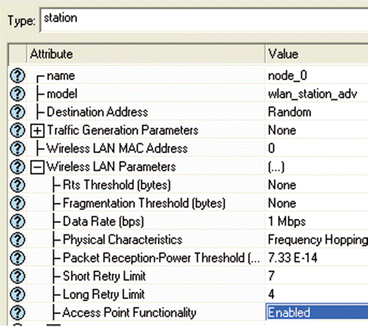

  

  Enabled the access point functionality for node 0

5.9.3 Select the Statistics

To test the performance of the network in our DCF scenario, we collect some of the available statistics as follows:

• 1. Right-click anywhere in the project workspace and select Choose Individual Statistics from the pop-up menu.

• 2. In the Choose Results dialog box, expand the Global Statistics and Node Statistics hierarchies → choose the five statistics, as shown in Fig. 5.22.

  Fig. 5.22

  

  The Chosen statistics results we want to show up

• 3. Click ok and then save your project.

5.9.4 Configure the Simulation

Here we will configure the simulation parameters:

• 1. Click on the Configure Simulation button.

• 2. Set the duration to be 10.0 min.

• 3. Click ok and then save your project.

5.9.5 Duplicate the Scenario

In the network we just created, we did not utilize many of the features explained in the overview. However, by default the distributed coordination function (DCF) method is used for the medium access control (MAC) sublayer. We will create three more scenarios to utilize the features available from the IEEE 802.11 standard. In the DCF_Frag scenario we will allow fragmentation of the MAC data units into smaller frames and test its effect on the network performance. The DCF_PCF scenario utilizes the point coordination function (PCF) method for the medium access control (MAC) sublayer along with the DCF method. Finally, in the DCF_PCF_Frag scenario we will allow fragmentation of the MAC data and check its effect along with PCF.

5.9.5.1 The DCF_Frag Scenario

• 1. Select Duplicate Scenario from the Scenarios menu and give it the name DCF_Frag → click ok.

• 2. Select all the nodes in the DCF_Frag scenario simultaneously → Right-click on anyone of them → Edit Attributes → Check the Apply Changes to Selected Objects check box.

• 3. Expand the hierarchy of the Wireless LAN Parameters attribute → Assign the value 256 to the Fragmentation Threshold (bytes) attribute, as shown in Fig. 5.23 → Click ok.

  Fig. 5.23

  

  DCF_Frag Scenario for node 8

• 4. Right-click on node_0 → Edit Attributes → Expand the Wireless LAN Parameters hierarchy and set the Access Point Functionality to Enabled as shown in Fig. 5.24 → Click ok.

  Fig. 5.24

  

  Enabled the access point functionality for node 0

5.9.5.2 The DCF_PCF Scenario

• 1. Switch to the DCF scenario, select Duplicate Scenario from the Scenarios menu and give it the name DCF_PCF → Click ok → Save your project.

• 2. Select node_0, node_1, node_3, node_5 and node_7 in the DCF_PCF scenario simultaneously → Right-click on anyone of the selected nodes → Edit Attributes.

• 3. Check Apply Changes to Selected Objects → Expand the hierarchy of the Wireless LAN Parameters attribute → Expand the hierarchy of the PCF Parameters attribute → Enable the PCF Functionality attribute, as shown in Fig. 5.25 → Click ok.

  Fig. 5.25

  

  Enabling PCF Parameters for node 0

• 4. Right-click on node_0 → Edit Attributes → Expand the Wireless LAN Parameters hierarchy and set the Access Point Functionality to Enabled, as shown in Fig. 5.26.

  Fig. 5.26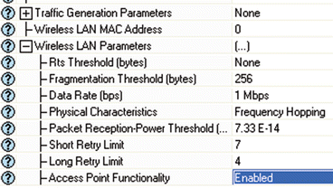

  

  Enabled the access point functionality for node 0

• 5. Click ok and save your project.

5.9.6 Run the Simulation

To run the simulation for the four scenarios simultaneously.

• 1. Go to the Scenarios menu → Select Manage Scenarios.

• 2. Click on the row of each scenario and click the Collect Results button. This should change the values under the Results column to < collect > shown in Fig. 5.27.

  Fig. 5.27

  

  Managing the Scenarios

• 3. Click ok to run the four simulations.

• 4. After the simulation of the four scenarios complete, click Close and then save your project.

5.9.7 View the Results

To view and analyze the results:

• 1. Select Compare Results from the Results menu.

• 2. Change the drop-down menu in the lower right part of the Compare Results dialog box from As Is to time-average → Select the Delay (sec) statistic from the Wireless LAN hierarchy as shown in Fig. 5.28.

  Fig. 5.28

  

  Comparing results

• 3. Click Show to show the result in a new panel. The resulting graph should resemble that shown in Fig. 5.29.

  Fig. 5.29

  

  Time average in WLAN delay (s)

• 4. Go to the Compare Results dialog → Follow the same procedure to show the graphs of the following statistics from the Wireless LAN hierarchy: Load (bits/s) and Throughput (bits/s). The resulting graphs should resemble Figs. 5.30 and 5.31.

  Fig. 5.30

  

  Time average in WLAN load (bits/s)

  Fig. 5.31

  

  Time average in WLAN throughput (bits/s)

• 5. Go to the Compare Results dialog box → Expand the Object Statistics hierarchy → Expand the Office Network hierarchy → Expand the hierarchy of two nodes. One node should have PCF enabled in the DCF_PCF scenario (e.g., node_3) and the other node should have PCF disabled (e.g., node_2) → Show the result of the Delay (sec) statistic for the chosen nodes. The resulting graphs should resemble Figs. 5.32 and 5.33.

  Fig. 5.32

  

  Time average in WLAN delay (s) for node 3

  Fig. 5.33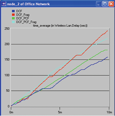

  

  Time average in WLAN delay (s) for node 2

• 6. Repeat step 5 above but for the Retransmission Attempts (packets) statistic. The resulting graphs should resemble Figs. 5.34 and 5.35.

  Fig. 5.34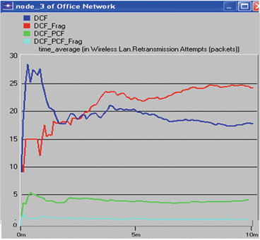

  

  Time average in WLAN retransmission line attempts (packets) for node 3

  Fig. 5.35

  

  Time average in WLAN retransmission line attempts (packets) for node 2

• 7. Close all graphs and the Compare Results dialog box → Save your project.

More information about Opnet can be found in [31].

5.10 NS2

The Network Simulator version 2 (NS2) is targeted at networking. It is object-oriented, discrete event driven network simulator. It was developed at UC Berkeley written in C++ language and it uses Object-oriented extension of Tool command language (OTcl). These two different languages are used for different purposes in NS2 as shown in Table 5.3 and more information about NS2 can be found in [32, 33].

Table 5.3 Use of OTcl and C++

Figure 5.36 shows the process of network simulation in NS2. The simulation using NS2 can carry two levels: first level is based on configuration and construction of OTcl, and second level, is based on OTcl and C++. It is essential for NS2 to be upgraded or modified to add the required elements when the module resources needed do not exist. Therefore, the split object model of NS2 is used to add a new C++ class and an OTcl class, and then program the OTcl scripts to implement the simulation [34]. The class hierarchies of C++ and OTcl languages can be either stand alone or linked together using an OTcl/C++ interface called TclCL [32].

Fig. 5.36

The simulation process of NS2 [34]

There are three components for whole network simulation using NS2 [35]. First, modifying the source code. This step is used only when there is a need to modify the source codes which requires programming and debugging from the users. Indeed, the OTcl codes need to be modified as the source codes due to that NS2 supports the OTcl and C++. Second, writing the Tcl/OTcl scripts of network simulations. In fact, in this step, it requires the user writing Tcl codes for describing the network topology types, defining nodes and network component attributes, controlling the network simulation process. Third, analyzing the network simulation results. This step requires the user to understand the structure of the NS2 Trace file and to be able to use some tools to check the outcome data and draw figures, etc. Figure 5.37 shows the flow chart for simulation in NS2. Although, the general architecture of the view of the NS2 for the general users can be presented in Fig. 5.38.

Fig. 5.37

The simulation flow chart of NS2 [35]

Fig. 5.38

The architectural view of NS2 [36]

NS2 is primarily useful for simulating LAN and WAN. It has the capability of supporting the simulations of unicast node and multicast node. It is complemented by Network Animator (NAM) for packet visualization purposes such as Fig. 5.39 for simulation topology of wireless network [37]. Indeed, NS2 is widely used network simulator that has been commonly used in education and research.

Fig. 5.39

Network animator interface (NAM) showing the simulation topology of wireless network [37]

NS2 has the following limitations [36]:

• 1. Large multi format outcome files, which require post processing.

• 2. Huge memory space consumption due to a very large output file.

• 3. Relatively slow.

• 4. Lack of built-in-QoS monitoring modules.

• 5. Lack of user friendly visual output representation.

• 6. Requires the users to develop tools by themselves.

5.11 Criteria for Language Selection

There are two types of factors that influence the selection of the special-purpose language an analyst uses in his simulation. One set of factors is concerned with the operational characteristics of the language, while the other set is related to its problem-oriented characteristics [38, 39].

In view of the operational characteristics of a language, an analyst must consider factors such as the following:

• 1. the analyst’s familiarity with the language;

• 2. the ease with which the language can be learned and used if the analyst is not familiar with it;

• 3. the languages supported at the installation where the simulation is to be done;

• 4. the complexity of the model;

• 5. the need for a comprehensive analysis and display of simulation results;

• 6. the language’s provision of good error diagnostics;

• 7. the compiling and running time efficiency of the language;

• 8. the availability of well written user’s manual;

• 9. the availability of support by a major interest group; and

• 10. the cost of installation, maintenance, and updating of the language.

In the view of the characteristics of the language and those of the problems the analyst will most likely encounter, the following factors should be considered:

• 1. time advance methods;

• 2. random number and random variate generation capabilities;

• 3. the way a language permits the analyst to control the sequence of subroutines that represent the state changes;

• 4. capability for inserting use-written subroutines; and

• 5. forms of statistical analyses that can be performed on the data collected during simulation.

No language is without some strong points as well as weak points. It is difficult to compare these languages because many important software features are quite subjective in nature. Everyone seems to have his own opinion concerning the desirable features of a simulation language, e.g. ease of model development, availability of technical assistance, and system compatibility. In spite of this difficulty, various attempts have been made to compare simulation languages based on objective criteria [22]. In general, GPSS and SLAM (which are FORTRAN-based) are easiest to learn.

SIMSCRIPT has the most general process approach and thus can be used to model any system without using the event-scheduling approach. This, however, may result in more lines of code than GPSS or SLAM. RESQ has features specially oriented toward computer and communication systems, but the terminology is strictly in terms of queueing networks.

5.12 Summary

• 1. This chapter has presented the basic concepts and definitions of simulation modeling of a system.

• 2. The emphasis of the chapter has been on discrete, stochastic, digital, software simulation modeling. It is discrete because it proceeds a step at a time. It is stochastic or nondeterministic because element of randomness is introduced by using random numbers. It is digital because the computers employed are digital. It is software because the simulation model is a computer program.

• 3. Because simulation is a system approach to solving a problem, we have considered the major stages involved in developing a model of a given system. These stages are model building.

• 4. Since simulation output is subject to random error, the simulator would like to know how close is the point estimate to the mean value μ it is supposed to estimate. The statistical accuracy of the point estimates is measured in terms of the confidence interval. The simulator generates some number of observations, say N, and employs standard statistical method to obtain the error estimate.

• 5. There are basically two types of languages used in simulation: multipurpose languages and special-purpose languages. The multipurpose or general-purpose languages include FORTRAN, BASIC, ADA, PASCAL, and C++. Special-purpose languages are meant to eliminate the major portion of the programming effort by providing a simulation-oriented framework about which a model is constructed in a simple fashion.

• 6. A brief introduction to two commonly used special-purpose, discrete simulation packages (NS2 and OPNET) is presented.

More information about simulation can be found in the references, including [40].

Problems

• 5.1 Define simulation and list five attractive reasons for it?

• 5.2 Generate 10,000 random numbers uniformly distributed between 0 and 1. Find the percentage of numbers between 0 and 0.1, between 0.1 and 0.2, etc., and compare your results with the expected distribution of 10 % in each interval.

• 5.3 (a) Using the linear congruential scheme, generate ten pseudorandom numbers with a = 1573, c = 19, m = 1000, and seed value X₀ = 89.

  (b) Repeat the generation with c = 0.

• 5.4 Uniformly distributed random integers between 11 and 30, inclusive, are to be generated from the random numbers U shown below. How many of the integers are odd numbers?

  0.2311	0.7919
  0.2312	0.9218
  0.6068	0.7382
  0.4860	0.1763
  0.8913	0.4057
  0.7621	0.9355
  0.4565	0.9169
  0.0185	0.4103
  0.8214	0.8936
  0.4447	0.0579

• 5.5 Generate 500 random numbers, exponentially distributed with mean 4, using uniformly distributed random numbers U. Estimate the mean and the variance of the variate.

• 5.6 Using the rejection method, generate a random variable from

  $$ f(x)=5{x}^2,\begin{array}{cc}\hfill \hfill & \hfill 0\le x\le 1\hfill \end{array} $$

• 5.7 (a) Using the idea presented in this chapter, generate 100 Gaussian variates with mean 3 and variance 2.

  (b) Repeat part (a) using MATLAB command randn.

  (c) By estimating the mean and variance, which procedure is more accurate?

• 5.8 The probability density function of Erlang distribution is

  $$ f(x)=\frac{\alpha^k{x}^{k-1}}{\Gamma (k)}{e}^{-\alpha x},\begin{array}{cc}\hfill \hfill & \hfill x>0,\alpha >0\hfill \end{array} $$

  where Γ(k) = (k − 1)! and k is an integer. Take k = 2 and α = 1. Use the rejection method to describe a procedure for generating random variates from Erlang distribution.

• 5.9 Write a computer program to produce variates that follow hyperexponential distribution, i.e.

  $$ f(x)= p\lambda {e}^{-\lambda x}+\left(1-p\right)\mu {e}^{-\mu x} $$

  Take p = 0.6, λ = 10, μ = 5.

• 5.10 Write a program to simulate the M/E_k/1 queueing system. Take k = 2. Compare the results of the simulation with those predicted by queueing theory.

• 5.11 A random sample of 50 variables taken from a normal population has a mean of 20 and standard deviation of 8. Calculate the error with 95 % confidence limits.

• 5.12 In a simulation model of a queueing system, an analyst obtained the mean waiting time for four simulation runs as 42.80, 41.60, 42.48, and 41.80 μs. Calculate the 98 % confidence interval for the waiting time.

• 5.13 Discuss the OPNET simulation results of Fig. 5.29 results?

• 5.14 Discuss the OPNET simulation comparison results of Figs. 5.30 and 5.31?

• 5.15 Discuss the OPNET simulation comparison results Figs. 5.32 through 5.35?

• 5.16 What are different purposes for C++ and OTcl languages in NS2?

• 5.17 What are the limitations of NS2?

References

S. V. Hoover and R. F. Perry, A Problem Solving Approach. New York: Addison-Wesley, 1989.
F. Neelamkavil, Computer Simulation and Modelling. Chichester: John Wiley & Sons, 1987, pp. 1-4.
M. H. MacDougall, Simulating Computer Systems: Techniques and Tools. Cambridge, MA: MIT Press, 1987, p. 1.
J. W. Schmidt and R. E. Taylor, Simulation and Analysis of Industrial Systems. Homewood, IL: R. D. Irwin, 1970, p. 5.
J. Banks and J. S. Carson, Discrete-event System Simulation. Englewood Cliffs, NJ: Prentice-Hall, 1984, pp. 3-16.
W. Delaney and E. Vaccari, Dynamic Models and Discrete Event Simulation. New York, Marcel Dekker, 1989, pp. 1,13.
G. S. Fishman, Concepts and Methods in Discrete Event Digital Simulation. New York: John Wiley & Sons, 1973, pp. 24-25.
W. J. Graybeal and U. W. Pooch, Simulation: Principles and Methods. Cambridge, MA: Winthrop Publishers, 1980, pp. 5-10.
T. G. Lewis and B. J. Smith, Computer Principles of Modeling and Simulation. Boston, MA: Houghton Mifflin, 1979, pp. 172-174.
M. N. O. Sadiku and M. Ilyas, Simulation of Local Area Networks. Boca Raton: CRC Press, 1995, pp. 44,45, 67-77.
A. M. Law and W. D. Kelton, Simulation of Modeling and Analysis. New York: McGraw-Hill, 2nd ed., 1991, pp. 420-457.
R. McHaney, Computer Simulation: a Practical Perspective. New York: Academic Press, 1991, pp. 91-95, 155-172.
H. Kobayashi, Modeling and Analysis: An Introduction to System Performance Evaluation Methodology. Reading, MA: Addison-Wesley, 1978
R. Jain, The Art of Computer Systems Performance Analysis. New York: John Wiley & Sons, 1991, pp. 474-501.
M.N.O. Sadiku and M. R. Tofighi, “A Tutorial on Simulation of Queueing Models,” International Journal of Electrical Engineering Education, vol. 36, 1999, pp. 102-120.
M. D. Fraser, “Simulation,” IEEE Potential, Feb. 1992, pp. 15-18.
M. H. Merel and F. J. Mullin, “Analytic Monte Carlo error analysis,” J. Spacecraft, vol. 5, no. 11, Nov. 1968, pp. 1304 -1308.
A. J. Chorin, “Hermite expansions in Monte-Carlo computation,” J. Comp. Phys., vol. 8, 1971, pp. 472 -482.
G. S. Fishman, Concepts and Methods in Discrete Event Digital Simulation. New York: John Wiley & Sons, 1973, pp. 92-96.
G. Gordon, “A General Purpose Systems Simulation Program,” Proc. EJCC, Washington D.C. New York: Macmillan, 1961.
J. Banks, J. S. Carson, and J. N. Sy, Getting Started with GPSS/H. Annandale, VA: Wolverine Software, 1989.
Minuteman Software: GPSS/PC Manual. Stow: MA, 1988.
B. Schmidt, The Simulator GPSS-FORTRAN Version 3. New York: Springer Verlag, 1987.
H. M. Markowitz, B. Hausner, and H. W. Karr, SIMSCRIPT: A Simulation Programming Language. Englewood Cliffs, NJ: Prentice-Hall, 1963.
P. J. Kiviat, R. Villaneuva, and H. M. Markowitz, The SIMSCRIPT II Programming Language. Englewood Cliffs, NJ: Prentice-Hall, 1968.
A. A. B. Pritsker, The GASP IV Simulation Language. New York: John Wiley & Sons, 1974.
A. A. B. Pritsker, Introduction to Simulation and SLAM II. New York: John Wiley & Sons, 2nd ed., 1984.
J. F. Kurose et al., “A graphics-oriented modeler’s workstation environment for the RESearch Queueing Package (RESQ),” Proc. ACM/IEEE Fall Joint Computer Conf., 1986.
I. Katzela, Modeling and Simulation Communication Networks. Upper Saddle River, NJ: Prentice Hall, 1999.
E. Aboelela, Network Simulation Experiments Manual. London, UK: Morgan Kaufmann, 2008, pp. 173–184.
T. Issarikakul and E. Hossain, “Introduction to Network Simulator NS2. Springer, 2009.
L. Fan and L. Taoshen, “Implementation and performance analyses of anycast QoS routing algorithm based on genetic algorithm in NS2,” Proceedings of Second International Conference on Information and Computing Science, 2009, pp. 368 – 371.
S. Xu and Y. Yang, “Protocols simulation and performance analysis in wireless network based on NS2,” Proceedings of International conference on Multimedia Technology (ICMT), 2011, pp. 638 – 641.
M. J. Rahimi et al., “Development of the smart QoS monitors to enhance the performance of the NS2 network simulator,” Proceedings of 13 th International Conference on computer and Information Technology, 2010, pp. 137-141.
R. Huang et al., “Simulation and analysis of mflood protocol in wireless network,” Proceedings of International Symposium on Computer Science and Computational Technology, 2008, pp. 658-662.
W. J. Graybeal and U. W. Pooch, Simulation: Principles and Methods. Cambridge, MA: Winthrop Publishers, 1980, p. 153.
J. R. Emshoff and R. L. Sisson, Design and Use of Computer Simulation Models. London: Macmillan, 1970, pp. 119-150.
D. Maki and M. Thompson, Mathematical modeling and Computer Simulation. Belmont, CA: Thomson Brooks/Cole, 2006, pp. 153-211.
Author information
Authors and Affiliations