Resilience of Wireless Mesh Networks

Abstract

This chapter presents a case study on resilient routing in Wireless Mesh Networks (WMNs) commonly formed by stationary mesh routers interconnected by wireless links. High-frequency communications (e.g., using the 71–86 GHz band) is the reason for the vulnerability of WMNs to weather-based disruptions, particularly to intensive precipitation. Therefore, heavy rainfalls may seriously reduce (or even completely degrade) the available link capacity in a given area. In this context, this chapter provides a set of measures of WMN resilience to region-based disruptions and proposes a transmission scheme that allows the preparation of the WMN topology to adverse weather conditions in advance by using the dynamic antenna alignment features according to forecasts of heavy rainfalls.

The second case study considered in this book refers to Wireless Mesh Networks (WMNs) formed by stationary mesh routers organized in a mesh topology [3, 22], providing transportation of flows originating from mesh clients (with little or no mobility). As presented in Fig. 9.1, WMN nodes have mesh capability, meaning their functioning is not restricted only to local data transmission. Instead, they can also relay information belonging to flows from other WMN nodes in a multi-hop fashion [18, 25]. If equipped with necessary functionality at specific nodes (i.e., gateways), WMNs may also be utilized to provide connectivity with external networks, e.g., the Internet [5, 8, 68].

Fig. 9.1

Example architecture of a Wireless Mesh Network including wireless mesh routers, mesh clients, and gateway routers

Most WMN architectures are based on the IEEE 802.11 standard, defining how wireless devices can be mutually interconnected to create a mesh network [26]. Compared to Wi-Fi solutions, the mesh structure of these networks implies a substantial enhancement in terms of the coverage area, connectivity, and scalability improvement, as well as simplifying deployment and maintenance activities [18, 68]. WMN end users are also provided with single-domain connectivity instead of switching between Wi-Fi hot-spots. It has been proved that the grid organization of WMN nodes provides up to 50% higher throughput than a random node placement [68].

Due to the utilization of the 71–86 GHz band [29, 39, 66], as well as highly directional antennas, the effective transmission rate can be as high as 1–10 Gb/s per millimeter-wave link with a transmission range of at least several kilometers [64, 72]. Therefore, WMNs can be seen as a promising alternative to wired local or even metropolitan area networks providing the last few miles of connectivity, especially in sparsely populated rural areas [22, 42].

It is also possible to equip each WMN router with MIMO technology (i.e., multiple-input multiple-output) utilizing multiple orthogonal channels [8]. This, in turn, leads to a further substantial increase in the network capacity [31, 71]. MIMO transmission is essential in urban areas encountering signal distortions, where such systems help amplify and rebuild signal levels, while directional antenna settings visibly reduce interference between neighboring channels [68]. What is similarly essential is that WMNs can provide connectivity among users without direct Line of Sight (LOS) links.

WMNs have also been shown to offer low connection costs in the backhaul area [8]. That is why using WMN solutions (e.g., instead of applying the fiber optic technology) is well justified for economic and practical reasons. It mainly refers to mobile operators not having their own fiber infrastructure, who otherwise would have to either deploy their own fiber network (which is very expensive in rural areas [20]) or try to lease capacity from other network providers. Deployment of WMNs has also been proposed to obtain affordable access networks for underdeveloped regions [42].

In the last decade, many research teams have been addressing the problems of capacity planning, placement of WMN nodes, routing, channel assignment, power control, topology control, etc. These problems are indeed very closely linked due to the nature of wireless interference. Therefore, when designing a WMN network, a joint consideration of these problems provides much better results in practice than in the case of a separate analysis. A comprehensive overview of joint design problems is presented in [42].

Several WMN installations are already in use in Europe, Australia, and the USA [17], deployed using equipment provided by, e.g., TerraNet, ArubaNetworks, or Motorola [4, 37, 62]. Example WMN architectures include city-wide (or cam-pus-wide) networks in Las Palmas, Spain and Corpus Cristi [65], Cambridge, Massachusetts, USA [68], Houston, USA [49], Oulu, Finland [59], Madison, USA [69], or Dartmouth, USA [24], with the number of nodes ranging from tens to hundreds, and the area of coverage measured in tens of square kilometers.

Apart from inheriting the typical characteristics of the general ad hoc networking concept (i.e., decentralized design, distributed communications), WMNs are known to exhibit characteristics that are novel in the wireless context but rather typical to wired networks, i.e., stationary nodes, no LOS connectivity, high capacity, and no limitations referring to node energy consumption [42].

Considering the transmission of information, we can even say that WMNs possess the most wired network characteristics, with the only apparent exception being the time-varying link stability. Therefore, applying the hop count metric for routing purposes in WMNs is inefficient (as shown in [13]). To respond to the dynamic characteristics of WMN links, several routing metrics have been proposed, the most important ones including the expected transmission count (EXT) [12], expected transmission time (ETT) [16], a metric of interference and channel switching (MIC) [70], or multichannel routing (MCR) [32]. They were designed to support WMN routing algorithms, e.g., AODV-ST [46], opportunistic Ex-OR [9], multipath routing [19], geographic routing [33], hierarchical routing [48], or multi-radio routing [32].

However, by incorporating the mentioned metrics into either a single-path or multipath routing [18], the impact of time-varying disruptions leading to partial/complete degradation of the effective capacity of WMN links can be reduced only in a reactive way. Proactive protection against failures (commonly known to achieve better performance, e.g., concerning the reduction of lost traffic after failures) is a relatively new research direction for WMNs. The problem is indeed essential since independent of the cause of failure (whether the result of an accident, forces of nature, or an intentional attack [63]), data and revenue losses encountered at high transmission rates of several Gb/s may undoubtedly be severe.

This chapter focuses on the failures of both WMN nodes and links. In particular, failures of WMN links can be covered by failure scenarios of the respective incident nodes (the topic addressed in Sect. 9.1). Failures of WMN links are commonly transient (i.e., not observed after the interval of a negative factor duration).

Although a significant part of the research is related to scenarios of isolated random failures of single nodes resulting from software errors or physical faults [1], such an assumption is improper for WMNs in many realistic scenarios. Example cases comprise natural disasters like earthquakes, volcano eruptions, tornadoes, or malicious human activities, including, e.g., bomb explosions [35], resulting in spatial correlation of failures of WMN nodes. WMN links are, in turn, very vulnerable to heavy precipitation, responsible for a remarkable signal attenuation.

In such cases, it is commonly assumed that the extent of negative outcomes depends on the characteristics of a particular event, with the major factor being the distance of a network element from the failure epicenter. This, in turn, gives rise to the region failure scenario [30, 38, 51, 52] addressing simultaneous failures of multiple nodes located close enough to suffer from the results of the event. Following [52], regions of failure can be defined concerning either network topology or geometry. The latter approach, i.e., a geometrical representation of a failure region determined by a circular radius area, shown in Fig. 9.2, is mainly used due to the predominant role of a node distance from the event epicenter [51, 52].

Fig. 9.2

Example of a failure region: dark gray circle centered at the epicenter of disruptions, and characterized by a given radius $\hat {\hat {r}}$, represents the area of possible failures of WMN nodes

In particular, to the best of our knowledge, no survivability measures are available to evaluate the performance of WMNs under region failures leading to simultaneous failures of multiple WMN nodes (as well as related links). Also, very few proposals refer to proactive protection of WMN flows against link failures. To provide the respective solutions, Sect. 9.1 introduces the appropriate survivability measures for WMNs, while Sect. 9.2 introduces a new approach to proactive protection against weather-based region disruptions based on automatic antenna alignment features. Section 9.3 concludes this chapter.

1 Measures of Wireless Mesh Networks Survivability

Due to the dependency of region-based failures on multiple characteristics, region failures need a detailed evaluation concerning their influence on the ratio of WMN performance degradation (e.g., measured in terms of the fraction of flow surviving failures of WMN nodes located inside a given failure region).

In this section, we present our approach to WMN regional failure assessment from [45] based on three introduced measures of WMN survivability for a circular region failure scenario under the random location of failure epicenters, i.e.:

• Region failure survivability function (RFS) being the cumulative probability of all region failure scenarios $\delta$ occurrence, for which at least $\psi$ percent of flows are successfully served after failures

• p-fractile region failure survivability function (PFRS), providing information on total flow reduction to at most $\psi$ percent after a failure at certain probability p

• Expected percentage of total flow delivered after a region failure as a function of region radius $\hat {\hat {r}}$ (EPFD)

Apart from providing a means of assessment of a given WMN to region disruptions, these measures are also proposed to enable comparisons of characteristics between different WMNs. To the best of our knowledge, besides our methodology from [45], no other relevant techniques are available in the literature appropriate for measuring the vulnerability of WMNs to regional failures of differentiated radiuses $\hat {\hat {r}}$ of failure regions.

The methodology of network survivability evaluation is well-established concerning wired networks (see, e.g., [21, 47, 53, 55, 61, 67]). Only a few proposals are available for wireless networks focusing, e.g., on the connectivity of network topology as a measure of fault tolerance [50]. Connectivity can be generally used to provide a binary answer to whether the network is k-connected, i.e., able to provide transmission continuity after a simultaneous failure of k-1 nodes. This idea has been extended to cover, e.g., average connectivity [7], distance connectivity [6], or path connectivity [23].

However, most existing proposals for WMN evaluation are unsuitable for a regional failure scenario with faults assumed to occur only in bounded areas. To address this problem, the respective region-based connectivity was proposed (see, e.g., [35, 50,51,52]). Concerning the scenario of circular failure regions, we can distinguish the models of:

• Deterministic failures (e.g., the single circular model from [52]), where any node located within the failure region is assumed to always fail with probability 1.

• Probabilistic failures with a probability of a node failure due to a disruptive event depending on the node distance from the failure epicenter [35]. This failure probability is assumed to decrease when the node distance from the failure epicenter increases.

Probabilistic models seem to provide more accurate results due to the common nondeterministic characteristics of natural disasters or attacks, resulting in failures of nodes located within failure regions with a certain probability. It is worth noting that available probabilistic approaches are not limitation-free. For instance, in [35], the size of a failure region (given by radius $\hat {\hat {r}}$) is assumed to be constant. Another constraint in [35] is that the probability of a node failure (even though decreasing with the increase of a node distance from the failure epicenter) is constant in each i-th area between two consecutive concentric annuluses (see Fig. 9.3a), which results in over- or underestimating the node failure probability values in some areas.

Fig. 9.3

Visualization of region failure probabilities: (a) from [35], and (b) the proposed one

Considering proposals of WMNs characteristics evaluation under region failures, several approaches have been introduced (e.g., [50,51,52]) to determine whether transmission in WMNs is possible between pairs of non-faulty nodes. To the best of our knowledge, our proposal described in this section is the first one to introduce the WMN survivability measures for the case of varying region radiuses $\hat {\hat {r}}$, and using the continuous function of node failure probability (see Fig. 9.3b and Eq. 9.3) that covers the models from [35, 52] as special cases.

It is worth noting that similar survivability measures have been proposed in the literature so far only for random failure scenarios in wired networks (see, e.g., [36]). However, they were designed for failures of network elements assumed to be statistically independent and equally probable, which is entirely in contrast to characteristics of WMN regional failures.

In the remaining part of this section, we first present details of the assumed network model (Sect. 9.1.1), followed by the proposed measures to evaluate the vulnerability of WMNs to regional failures (Sect. 9.1.2). Next, we describe the methodology of WMN survivability evaluation (Sect. 9.1.3) and comment on the results of simulations performed, for the example network topologies (Sect. 9.1.4).

1.1 Network Model

In this chapter, we model the WMN topology by graph $G= (N,A)$, where N represents the set of WMN stationary nodes (following [42]), while A denotes the set of directed arcs $a_h=(i, j)$. Each WMN link between neighboring nodes i and j is represented by two arcs in opposite directions. Additional information refers to the location of each node n defined by coordinates ($\bar {x}_n$,$\bar {y}_n$). Despite the assumed stationary characteristics of network nodes, the methodology of network assessment presented in this section can also be easily adapted to the case of mobile nodes (if performed concerning the instant topology of a network at time t).

The available capacity of any WMN link is a result of multiple factors, the most important ones being medium access protocol implementation, interchannel interference implied by the respective link scheduling algorithm [11, 18], or time-varying factors including, e.g., weather-based disruptions caused by heavy rain falls (general propagation conditions) [27]. Since the effective capacity of any WMN link changes over time, it is reasonable to perform evaluations at a given time t, i.e., assuming that the capacity of arc $a_h$ is equal to $c_h$(t).

The set of demands D consists of demands $d_r$ defined by ordered triples ($s_r$, $t_r$, $c_r$), i.e., described by source and destination nodes $s_r$ and $t_r$, and the demanded capacity $c_r$.

Two matrices are used in our model description: $A_{nn}$ and $D_{nn}$. Node-to-node incidence matrix $A_{nn}$ provides information on connectivity with elements defined by formula (9.1).

$$\displaystyle \begin{aligned} a_{i,j} = \begin{cases} 1, & \text{if arc }a_h=(i,j) \in A_{nn}\\ 0, & \text{otherwise} \end{cases} {} \end{aligned} $$

(9.1)

Information about aggregate capacities required for flows (commodities) between given pairs of end nodes is stored in elements $d_{s,t}$ of matrix $D_{nn}$.

$$\displaystyle \begin{aligned} d_{s,t}=(s_r, t_r, c_r) {} \end{aligned} $$

(9.2)

During evaluations, the location of a failure epicenter is chosen at random (i.e., following the uniform distribution function of failure epicenter coordinates) within the smallest rectangular area containing the network. We assume a probabilistic failure scenario with a disruptive event affecting nodes localized within a given radius $\hat {\hat {r}}$ from the failure epicenter. In particular, in our model:

• Radius $\hat {\hat {r}}$ of a failure circular region is uniformly distributed over (0, $\hat {\hat {r}}_{\text{max}}$), where $\hat {\hat {r}}_{\text{max}}$ is equal to half of the largest Euclidean distance between any two nodes in the network;

• Probability P($\hat {\hat {r}}_n$) of node n failure is given by a decreasing continuous function of the distance $\hat {\hat {r}}_n$ between node n and the failure epicenter (see Fig. 9.3b and Eq. 9.3). P($\hat {\hat {r}}_n$) is thus the generalization of the respective formula from [35].

$$\displaystyle \begin{aligned} P(\hat{\hat{r}}_n) = \begin{cases} -\frac{\hat{\hat{r}}_n}{\hat{\hat{r}}}+1 =-\frac{\sqrt{(\bar{x}_n-\bar{x})^2+(\bar{y}_n-\bar{y})^2}}{\hat{\hat{r}}}+1& \text{if } \hat{\hat{r}}_n \leq \hat{\hat{r}}\\ 0, & \text{otherwise} \end{cases} {} \end{aligned} $$

(9.3)

where:

($\bar {x}_n$,$\bar {y}_n$):

are coordinates (location) of node n;

($\bar {x}$,$\bar {y}$):

are coordinates (location) of the failure epicenter;

$\hat {\hat {r}}$:

is the radius of a failure region;

$\hat {\hat {r}}_n$:

is the distance of node n from the failure epicenter.

It is reasonable to introduce the WMN node failure probability function as given in Eq. 9.3 since, following [35], the negative impact of real physical attacks (e.g., bomb explosions or electromagnetic pulse (EMP) attacks), as well as natural disasters (earthquakes, floods, etc.), attenuates gradually with the increase of the distance of WMN nodes from the failure epicenter. As given in [35], the maximum value of node failure probability can be assumed to be equal to 1 for locations of nodes matching exactly the failure epicenter. Its lowest value of 0 is, in turn, attributed to nodes located at a distance $\hat {\hat {r}}_n$ not smaller than $\hat {\hat {r}}$ from the failure epicenter.

It is worth noting that this gradual attenuation of P($\hat {\hat {r}}_n$) values with the increase of the distance $\hat {\hat {r}}_n$ can be disturbed by several environmental factors, e.g., topography or node protection characteristics. However, if we neglect them to simplify the analysis (following [35]), the decrease of probability P($\hat {\hat {r}}_n$) of node n failure becomes linear with the increase of node n distance from the epicenter of disruptions, as introduced in Eq. 9.3.

1.2 Proposed Measures to Evaluate the Survivability of WMNs

The following notation is used in the remaining part of Sect. 9.1:

$\delta$:

a regional failure scenario given by the set of nonoperational nodes (after the outage)

$P(\delta )$:

probability of occurrence of a failure scenario $\delta$

$\Psi (\delta )$:

random variable referring to the percentage $\psi$ of flows delivered in scenario $\delta$

$p_{\Psi }(\psi )$:

probability density function of percentage $\psi$ of flows surviving the region failure, defined by Eq. 9.4

$$\displaystyle \begin{aligned} p_{\Psi}(\psi) = \sum_{\delta:\Psi(\delta)=\psi}^{} P(\delta) {} \end{aligned} $$

(9.4)

We introduce three measures of WMN survivability for a regional failure scenario, i.e.:

• 1. Region failure survivability function (RFS) of the percentage $\psi$ of flows successfully transmitted after regional failures:

  $$\displaystyle \begin{aligned} RFS(\psi) = \sum_{\delta:\Psi(\delta)\geq\psi}^{} P(\delta)=1-\sum_{\delta:\Psi(\delta)<\psi}^{} P(\delta)=1-cdf(\Psi) {} \end{aligned} $$

  (9.5)

  As given in Eq. 9.5, RFS($\psi$) is defined for any value of $\psi$ as the cumulative probability of all region failure scenarios $\delta$ (i.e., for differentiated radiuses $\hat {\hat {r}}$ of failure regions) for which at least $\psi$ percent of flows survived the failure. It can be thus expressed as the reverse cumulative distribution function of $\Psi$. Although Eq. 9.5 shows some similarities with the respective one from [36] for wired networks, the calculation of P($\delta$) values is entirely different.

• 2. p-fractile region survivability (PFRS):

  $$\displaystyle \begin{aligned} PFRS(p) =\text{inf}\left\{ \psi: \sum_{\delta:\Psi(\delta)<\psi}^{} P(\delta)=p\right\} {} \end{aligned} $$

  (9.6)

  Following formula (9.6), the value of p-fractile region survivability refers to the minimum percentage $\psi$ of flows delivered after a regional failure, for which the probability of not exceeding this value is equal to p. PFRS thus returns useful information about probability p that the total flow is reduced to at most $\psi$ percent after the failure.

  Since RFS and PFRS measures do not depend directly on the radius $\hat {\hat {r}}$ (i.e., they allow radius $\hat {\hat {r}}$ to take any value from (0, $\hat {\hat {r}}_{\text{max}}$) interval), they are designed to give general information on network vulnerability to regional failures. These measures are thus appropriate if the objective is to analyze the performance of WMNs independent of the failure region size $\hat {\hat {r}}$. However, the information they provide is of different types.

  For instance, if for a given WMN, at least $\psi$ percent of traffic should be delivered (e.g., because such a portion of traffic is considered to be critical based on the Service Level Agreement), then RFS is the appropriate one to provide information about probability p of fulfilling this requirement under regional failures independent of size $\hat {\hat {r}}$ of the failure region. Naturally, the greater the value of p, the better performance of a network can be achieved.

  PFRS is, in turn, a suitable measure for a network operator to determine, given the respective probability p, what is the upper bound on the fraction $\psi$ of flow surviving a regional failure. It is, therefore, useful to give information on the probability that not all of the $\psi$ percent of flows (e.g., referred to as the critical flow) will survive the regional failure, i.e., in statements like: “with probability 0.7, the total flow will be reduced to at most 80% of the traffic served before the regional failure.”

  The following EPFD function is introduced to obtain detailed characteristics of a WMN performance related to particular radiuses $\hat {\hat {r}}$ of failure regions.

• 3. Expected percentage of total flow delivered after a failure (EPFD) as a function of region radius $\hat {\hat {r}}$:

  $$\displaystyle \begin{aligned} EPFD(\hat{\hat{r}}) = \sum_{\psi}^{} \psi \cdot p_{\psi}(\psi, \hat{\hat{r}}) {} \end{aligned} $$

  (9.7)

  where:

  $\hat {\hat {r}}$:

  is the radius of a failure region;

  $p_{\psi }(\psi , \hat {\hat {r}}$):

  is the probability density function of $\Psi$ defined for failure region of radius $\hat {\hat {r}}$.

  $$\displaystyle \begin{aligned} p_{\psi}(\psi, \hat{\hat{r}})= \sum_{\delta:\Psi(\delta)=\psi;\hat{\hat{r}}}^{} P(\delta) {} \end{aligned} $$

  (9.8)

  EPFD($\hat {\hat {r}}$) is defined in Eq. 9.7 as the expected value of the percentage of flows to survive failures of nodes bounded in circular regions, i.e., derived using the probability density function $p_{\psi }(\psi , \hat {\hat {r}})$ obtained for failure regions of a given radius $\hat {\hat {r}}$ (see formula (9.8)).

  Concerning scenarios of EPFD measure utilization, it can be helpful in any performance analysis/comparison of WMNs under regional failures being the result of, e.g., natural disasters (like floods or volcano eruptions), for which the failure region is commonly expected to have a circular shape defined by a given radius $\hat {\hat {r}}$. Another application of EPFD measure would be, e.g., when expecting failures confined to a certain region characterized by radius $\hat {\hat {r}}$ (e.g., incoming flood), to predict its impact on WMN performance, being helpful to take preventive actions.

The later part of this section provides information on how to utilize the three introduced measures to evaluate the vulnerability of WMNs to regional failures and how to use them to compare performance characteristics of different topologies.

1.3 Method of a WMN Survivability Evaluation

This section explains our methodology of WMN survivability characteristics evaluation under regional failures. In particular, we focus on determining the introduced RFS, PFRS, and EPFD characteristics, for example, WMNs.

Proposed measures are derived from the auxiliary function F[$\psi$] providing information on the frequency a given percentage of flows ($\psi \in \{0,1,\ldots , 100\}$) is successfully delivered after regional failures. F[$\psi$] values can be collected for a given WMN based on network performance observations after consecutive disruptive events implying failures of WMN nodes confined to given regions. However, deriving any characteristics based on real-life experiments is time-consuming and practically impossible due to rather long inter-failure time intervals (typically measured in months/years).

In this section, an iterative procedure is presented to simulate consecutive region failures in a way that eliminates the inter-failure time. In this way, it is possible to analyze the performance of existing networks and predict the survivability characteristics of planned (i.e., non-deployed) WMNs using information related to the abstract WMN topology and estimated demand volumes.

The 13-step procedure to determine F[$\psi$] values for a single set of demands is given in Fig. 9.4. The most essential input information is related to the following:

• Topology of existing/planned WMN defined by a graph G with sets N and A of nodes and directed arcs, representing network nodes and links, respectively

  Fig. 9.4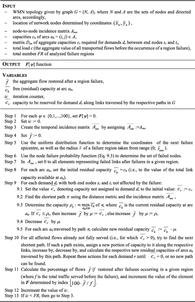

  

  Method of determining F($\psi$) values

• Location of network nodes defined by coordinates ($\bar {x}_n$,$\bar {y}_n$)

• Demands $d_r$, given by the requested throughput $c_r$, and source and destination nodes $s_r$ / $t_r$

After initialization, Steps 1–2, the purpose of each iteration given by Steps 3–13 is to obtain the percentage $\psi$ of flows delivered after failures of WMN nodes occurring in a given failure region. The coordinates of each failure epicenter and the radius $\hat {\hat {r}}$ of a failure region are defined as random values by the continuous uniform distribution function (following [35]).

In particular, it implies that in each iteration of the analyzed procedure:

• The location of a failure epicenter is chosen at random within the smallest rectangular area containing the WMN topology, using the continuous uniform distribution function.

• Radius $\hat {\hat {r}}$ of a failure circular region is uniformly distributed over (0, $\hat {\hat {r}}_{\text{max}}$), with $\hat {\hat {r}}_{\text{max}}$ equal to half of the largest Euclidean distance between any two nodes in the network.

After the iteration initialization, Steps 3–5, Step 6 is to identify the set of failed nodes (based on formula (9.3)). To evaluate the percentage $\psi$ of flows delivered in a given regional failure scenario, for each flow with both end nodes being non-faulty, our method tries to find an alternate path of capacity $c_r$ (Steps 7–9). If the new path is found, but, due to link capacity limitations, it cannot be assigned the demanded capacity $c_r$, multipath routing is then applied to increase as much as possible the capacity assigned to demand $d_r$ after a regional failure (Step 10).

The percentage $\psi$ of flows successfully delivered after a failure is calculated in Step 11 based on the ratio of the aggregate flow $\hat {f}$ restored after the failure to the total flow f being transported before the failure (i.e., after finding the alternate paths for all demands in a given region failure scenario). Following Steps 12–13, the analysis is repeated until the number FR of failure regions is evaluated.

All three introduced functions (RFS, PFRS, and EPFD) are next derived based on F[$\psi$] values. In particular:

• RFS($\psi$) is calculated based on empirical probabilities of restoring $\psi$ percent of flows after failures (each such probability is obtained by dividing the respective value of F[$\psi$] by FR, i.e., by the total number of analyzed failure regions). According to formula (9.5), RFS($\psi$) is determined as the reverse cumulative distribution function of $\Psi$.

• PFRS(p) is obtained based on the cumulative distribution function of $\Psi$ (formula (9.6)).

• EPFD($\hat {\hat {r}}$) is calculated based on probability density functions $p_{\psi }(\psi , \hat {\hat {r}})$ found separately for each radius $\hat {\hat {r}}$ of a failure region using Eq. 9.7.

To find the optimal solution to the problem of determining a new set of paths in a capacity-constrained network after failures to maximize the amount of restored flows, the respective linear programming formulation of the problem (LP) is necessary [40]. However, due to its $\mathcal {N}\mathcal {P}$-completeness (see, e.g., [43]), the optimal solution can be found in a reasonable time using offline approaches only for small problem instances (e.g., for networks up to 12–15 nodes). Therefore, in the proposed method, calculating the alternate paths (Steps 9.2 and 10 in Fig. 9.4) is done using the heuristic approach based on Dijkstra’s algorithm [15] that is proved to have the polynomial computational complexity bounded in above by O($|N|^2$), where $|N|$ is the number of WMN nodes.

1.4 Analysis of Modeling Results and Conclusions

In this section, we evaluate the vulnerability of five example WMNs to region failures (i.e., N29, N29_2, N29_3, N44, and N59 networks from Fig. 9.5), utilizing the proposed survivability measures. The first three networks (presented in Fig. 9.5a–c are formed by 29 nodes located in 4000 $\times$ 10,000 m${ }^2$, 6000 $\times$ 6000 m${ }^2$, and 8000 $\times$ 8000 m${ }^2$ fields, respectively, connected by 68, 68, and 57 wireless links, respectively. The other two networks shown in Fig. 9.5d–e consist of 44 and 59 nodes (located in fields of 10,000 $\times$ 10,000 m${ }^2$), respectively, connected by 97 and 150 wireless links, respectively.

Fig. 9.5

Evaluated topologies of: N29 (a); N29_2 (b); N29_3 (c); N44 (d); and N59 (e) networks

It is worth noting that for the N29 network, due to visible differences between horizontal and vertical sizes of the rectangular area (4000 m and 10,000 m, respectively), this network is likely to obtain the worst results concerning the portion of flows surviving the regional failures (since for each network, the analyzed radiuses $\hat {\hat {r}}$ of failure regions were up to half of the largest Euclidean distance between any two nodes in the network).

When assessing the vulnerability of network flows to region disruptions, all transmission paths (both before and after failures) were calculated as the cheapest ones using the standard metric of distance [34, 41]. After failures, a reactive approach was utilized to redirect flows with survived end nodes. To provide the appropriate statistical analysis related to RFS, PFRS, and EPFD functions, the original values of F[$\psi$] were obtained as the aggregate ones, including all 100 investigated demand sets of a certain size. For each set of demands, failures related to $FR = 9000$ random regions were simulated.

Three simulation scenarios were considered. The first two, referred to as Scenarios A and B, were prepared to use the proposed measures to evaluate the characteristics of different WMNs under a similar network load. To achieve this, the sets of unicast transmission demands included 25% of randomly chosen node pairs. Scenario A was to verify characteristics of WMNs of the same size in terms of the number of nodes (i.e., N29, N29_2, and N29_3 networks consisting of 29 nodes), while Scenario B was aimed at evaluating networks covering a similar area (i.e., not necessarily comparable in terms of the number of nodes). Therefore, topologies analyzed in Scenario B included N29, N44, and N59.

Additional Scenario C was to verify the properties of our measures under differentiated loads of the N59 network. In particular, four sizes of demand sets (i.e., consisting of randomly chosen 25%, 50%, 75%, and 100% node pairs) were examined. The capacity $c_r$ of each unicast demand $d_r$ was assumed to be unitary.

Each network link offered 160 units of unitary capacity in each direction. Considering failure scenarios, radiuses $\hat {\hat {r}}$ of failure regions were uniformly distributed in range (0, $\hat {\hat {r}}_{\text{max}}$), where $\hat {\hat {r}}_{\text{max}}$ was equal to half of the largest Euclidean distance between any two network nodes. Statistical analysis of results was based on 95% confidence intervals. However, since the sizes of obtained intervals did not exceed 1% of the original values due to low visibility, they are not shown in Figs. 9.6–9.12.

Fig. 9.6

RFS($\psi$) function (Scenario A)

Region Failure Survivability (RFS)

Evaluation of the vulnerability of WMN topologies to regional failures using the RFS measure under the assumptions of Scenario A is presented in Figs. 9.6 and 9.7. Recall that the RFS measure, defined in Eq. 9.5, was introduced to evaluate the probability that at least $\psi$ percent of flows survive after a regional failure.

Fig. 9.7

RFS($\psi$) function (Scenario B)

Fig. 9.8

PFRS(p) function (Scenario A)

As presented in Figs. 9.6 and 9.7, with the increase of $\psi$, RFS starts decaying from the value of 1 (since, independent of the network topology, the probability of reducing the total flow to at least 0% is equal to 1). When comparing RFS characteristics for any two network topologies, greater values of RFS for any value of $\psi$ imply a better network performance after a failure (since they reflect a greater chance of total flow reduction to at least $\psi$ percent after a failure).

The general conclusion that follows from Figs. 9.6 and 9.7 is that better results concerning network survivability characteristics under regional failures are attributed to WMN networks with RFS functions driven by a slower decay with the increase of $\psi$ (i.e., for which independent of $\psi$ parameter, RFS values are higher). For instance, as shown in Fig. 9.6, the N29 network (for which its horizontal and vertical sizes are remarkably different) is outperformed by the N29_2 and N29_3 networks (located inside a square area) in Scenario A. In the same way, the N44 and N59 networks turned out to outperform the N29 network in Scenario B (Fig. 9.7).

p-Fractile Region Survivability (PFRS)

Figures 9.8 and 9.9 show evaluation of WMN survivability characteristics using the p-fractile region survivability (PFRS) measure for Scenarios A and B. Recall that PFRS (Eq. 9.6) is to provide information on probability p that the fraction of total flow delivered after regional failures will not exceed $\psi$ (Y axis on Figs. 9.8 and 9.9).

Fig. 9.9

PFRS(p) function (Scenario B)

Fig. 9.10

EPFD($\hat {\hat {r}}$) function (Scenario A)

For any WMN, it is thus better if, for any value of p, the upper bound on the portion $\psi$ of flow surviving the failure is higher. As shown in Figs. 9.8 and 9.9, independent of the network topology, PFRS values are consistently positively correlated with p. Generally, the lower the values of PFRS, the more vulnerable the network is to regional failures. Similar to results for the RFS measure, PFRS also showed that the N29 network has the worst properties among all analyzed WMNs in Scenarios A–B.

EPFD Function

Figures 9.10 and 9.11 show values of EPFD function obtained in Scenarios A and B. Recall that EPFD function is defined by formula (9.7) as the expected percentage of the total flow delivered after failures occurring in circular areas of a certain radius $\hat {\hat {r}}$. For any radius $\hat {\hat {r}}$, greater values of the EPFD function imply more network flows surviving the failures. As shown in Figs. 9.10 and 9.11, the N29 network obtained the worst characteristics also concerning EPFD measure (which is compliant with the respective RFS and PFRS characteristics from Figs. 9.6–9.9, respectively).

Fig. 9.11

EPFD($\hat {\hat {r}}$) function (Scenario B)

Fig. 9.12

Characteristics of (a) RFS($\psi$), (b) PFRS(p), and (c) EPFD($\hat {\hat {r}}$) functions for Scenario C (N59 network)

It is worth mentioning that none of the three measures depends on the network load (as shown in Fig. 9.12 for Scenario C). Therefore, they can be used to compare the characteristics of different WMN topologies.

In this section, we focused on evaluating the vulnerability of WMNs to region failures occurring in circular areas and introduced three measures for evaluating WMN survivability. The first two measures, i.e., region failure survivability function—RFS and p-fractile region survivability function—PFRS, were proposed to assess WMN vulnerability to regional failures independent of the radius $\hat {\hat {r}}$ of the failure region. The third measure—the expected percentage of total flow delivered after a region failure as a function of region radius $\hat {\hat {r}}$ (EPFD)—was, in turn, designed to evaluate WMN performance depending on the radius $\hat {\hat {r}}$ of a circular failure region.

Proposed measures were later utilized to evaluate the properties of three example topologies of WMNs. Simulation analysis confirmed that these measures provide adequate and consistent information on the vulnerability of WMN networks to regional failures. Since for all introduced measures, achieved characteristics did not depend on the network load, they can thus be utilized in comparisons of different WMNs.

2 A New Approach to the Design of Weather Disruption-Tolerant Wireless Mesh Networks

As discussed in the former part of this chapter, failures of WMN nodes/links may imply severe data losses. In this section, we focus on link failures and present the respective approach to survivable routing to improve the WMN performance under link failures. As stated in [57], WMN links are susceptible to weather disruptions, particularly precipitation. Heavy rain storms may cause high signal attenuation, remarkably reducing the available link capacity or implying a link failure, leading to instability problems of routing (i.e., route flapping).

The issue of survivable routing is well-researched concerning wired networks (see, e.g., [47, 55, 58, 61, 67]), in particular concerning the protection of WDM network flows ([47, 55, 56, 60]). Among a few proposals on routing resilience in wireless networks, we can mention reference [10] addressing shared medium problems and node mobility issues. However, these solutions cannot be directly applied to WMNs due to remarkably different characteristics. In particular, WMNs are commonly nonmobile and do not encounter contention problems (if equipped with directional antennas). Therefore, except for link stability issues, WMNs seem to share the most important characteristics with wired networks [27].

To protect flows against weather-based disruptions of WMN links, it seems reasonable to use information related to expected incoming rain storms (e.g., achieved from radar echo measurements) to predict the real shapes of signal attenuation regions. Based on this idea, two approaches were introduced in [27], namely XL-OSPF and P-WARP, to modify the link-state OSPF routing based on weather predictions. Both techniques utilize formulas (9.9)–(9.10) from [14], defining the dependency of signal attenuation on the rain rate.

(9.9)

(9.10)

where:

$\Omega$:

is the signal attenuation in dB;

$\Theta$:

is the length of the path over which the rain is observed;

$R_p$:

is the rain rate in mm/h;

$\alpha$, $\beta$:

are the numerical constants from [14].

• $u=\frac {\text{ln}(be^{\iota \vartheta })}{\vartheta }$,  $\ b=2.3R_p^{-0.17}$.

• $\ \iota =0.026-0.03\text{ln}R_p$, $\vartheta =3.8-0.6 \text{ln} R_{p}$.

In particular, XL-OSPF utilizes a special metric of link cost being proportional to the observed bit error rate (BER) of the link (which is justifiable due to the clear impact of signal attenuation on the effective BER, as well as on packet error rate—PER). This metric is utilized reactively to update the OSPF routing characteristics. However, such an approach is not straightforward to deploy since, in the Media Access Control (MAC) layer, there is no information on the actual BER between network nodes (it can be estimated using signal-to-noise ratio—SNR).

P-WARP, in turn, estimates the costs of WMN links using weather-based predictions of future conditions of links. This can be done at either one dedicated node or a subset of nodes capable of collecting the weather-related radar data.

In this section, we focus on reducing the signal attenuation level along millimeter-wave links in the presence of rain storms. In particular, in Sect. 9.2.1, we present in detail our method from [44] to perform in advance the periodic updates of a WMN topology following forecasts of heavy rain storms, using the functionality of a dynamic antenna alignment offered by several equipment vendors (see, e.g., [54]). Next, in Sect. 9.2.2, we describe the ILP model we proposed to obtain the optimal routing solution per the forecasted levels of signal attenuation at WMN links (that also returns the proper assignment of non-interfering channels to intersecting links). After that, in Sect. 9.2.3, we present the analysis of the problem’s computational complexity, followed by an evaluation of our approach characteristics (Sect. 9.2.4).

To the best of our knowledge, the protection of WMN links against weather-based regional failures has not been sufficiently researched so far. In particular, there is no other proactive approach that is based on periodic updates of a WMN topology.

2.1 Proposed Approach

The technique to protect WMN links against weather-based disruptions described here does not impose any modifications to the routing algorithm. Therefore, it can be used with practically any routing scheme, making our solution easily deployable. In particular, transmission paths are established based on conventional metric of link costs (e.g., the number of hops).

The main idea of our approach is to prepare the network for changing weather conditions by applying the periodic updates of WMN topology to improve the throughput during rain storms. We propose to perform consecutive updates of a WMN topology by employing dynamic antenna alignment features (offered by several equipment vendors) utilizing predictions related to future conditions of WMN links based on rain storm forecasts obtained from real echo rain maps. This, in turn, implies periodic creation (or deletion) of WMN links if low (or high) values of signal attenuation are expected for them, respectively.

The network is modeled in this section by graph $G{=}(N, A)$, similar to Sect. 9.1.1. In particular, any link between two neighboring nodes, i and j, is represented by two directed arcs $a_h{=}(i, j)$ and $a_{h'}{=}(j, i)$, respectively, and is assigned a given transmission channel from the set of available transmission channels. To focus on time-varying characteristics of WMN links, the definition of graph G is extended by:

• Ť denoting the lifetime of a network.

• $\vartheta$(Ť): A x Ť $\rightarrow$ {0, 1} function determining the existence of links at time t $\in$Ť.

• $\gamma$(Ť): A x Ť $\rightarrow$ $\mathcal {R}$ link cost function based on signal attenuation ratio at time t $\in$Ť (formulas (9.9)–(9.10)).

We assume the existence of a dedicated core node responsible for the alignment of antennas of all network nodes that has access to:

• The set of active network nodes and their locations

• Radar echo rain measurements (received periodically)

• Demands to provide transmission between WMN end nodes

The role of this core node is also to execute the procedure shown in Fig. 9.13. In particular, in Step 1 of this scheme, the estimated signal attenuation $\omega _h$ at each potential arc $a_h{=}(i, j)$ is determined using formulas (9.9)–(9.10). The action of Step 2 is to return a new configuration of WMN links. In particular, in the proposed scheme, $\omega _h$ values are used as link costs to obtain the set of the cheapest (in terms of signal attenuation) potential paths. If, in Step 2, a given link is not used by any path, it will not be present in the updated WMN topology.

Fig. 9.13

Proposed methodology of periodic updates of alignment of WMN antennas

In the method from Fig. 9.13, we propose to utilize the heuristic approach to proceed with Step 2, since the problem to determine the optimal alignment of WMN antennas with the objective to minimize the aggregate signal attenuation over all transmission paths, defined in Sect. 9.2.2, is $\mathcal {N}\mathcal {P}$-complete (as proved in Sect. 9.2.3). New alignment of antennas (Step 3) is expected every $\tau$ time units (as defined in Step 4).

It is worth recalling that metric $\omega _h$ is used in our approach only to update the alignment of antennas at WMN nodes. Routing is, in turn, performed using a conventional protocol with all its characteristics unchanged. This implies that the original metric of link costs (i.e., the one normally used by the routing algorithm) is utilized instead of $\omega _h$ values to obtain the real transmission paths.

2.2 ILP Formulation of Weather-Resistant Links Formation Problem (WRLFP)

The problem of determining the optimal alignment of WMN antennas (Step 2 from Fig. 9.13) to minimize the aggregate signal attenuation over all transmission paths at time t can be solved by determining the solution to the following ILP model. Symbols

G(N,A):

Graph representing a directed network.

N:

Set of network nodes; $|N|$ is the number of network nodes.

A:

Set of directed arcs; $|A|$ is the number of arcs.

h:

Arc index; h = 1, 2, ..., $|A|$.

D:

Set of demands; $|D|$ is the number of demands.

r:

Demand index; r = 1, 2, ..., $|D|$.

$L_h$:

Set of transmission channels available at arc $a_h$ = (i, j).

$1...\Lambda _h$:

Indices of transmission channels at arc $a_h$ = (i, j); ).

Constants

$s_r(t_r)$:

Source (destination) node of r-th demand.

$c_r$:

Capacity of r-th demand.

$c_h(t)$:

Estimated total capacity of arc $a_h$ = (i, j) at time t.

$\omega _h(t)$:

Estimated signal attenuation due to rain falls for arc $a_h$ = (i, j) at time t.

Variables

$x^{l}_{r,h}$:

Equals 1, if l-th channel is assigned for r-th demand path at arc $a_h$= (i, j); 0 otherwise.

Objective

It is to find the end-to-end transmission paths for all demands, minimizing the cost defined by formula (9.11).

(9.11)

where $\omega _h(t)$ is the cost of arc $a_h$ = (i, j) based on signal attenuation ratio at time t.

Constraints

• 1. Flow conservation rules (based on Kirchhoff’s law) for end-to-end paths:

  $$\displaystyle \begin{aligned} \sum_{l \in L_h}{}\sum_{\substack{h \in \{h:a_h = (n, j) \in A;\\ j=1, 2,..., |N|; j \neq n\}}}^{} x^{l}_{r,h} - \sum_{l \in L_h}{}\sum_{\substack{h \in \{h:a_h = (i, n) \in A;\\ i=1, 2,..., |N|; i \neq n\}}}^{} x^{l}_{r,h} =\begin{cases} 1, & \text{if }n= s_r\\ -1, & \text{if }n= t_r\\ 0, & \text{otherwise} \end{cases} {} \end{aligned} $$

  (9.12)

  where:

  $a_h{=}(n,j)$ denotes an arc incident out of node n; $a_h$=(i,n) refers to an arc incident into node n; r=1, 2,..., $|D|$; n=1,2,..., $|N|$.

• 2. On the finite capacity of arcs $a_h$ (i.e., to assure that the total flow assigned to arc $a_h$ will not exceed the maximum available capacity):

  

  (9.13)

• 3. On the selection of different channels to interfering links (at most one link from the set of interfering links can be assigned a given channel l):

  $$\displaystyle \begin{aligned} \sum_{r \in D}^{} x^{l}_{r,h} + \sum_{r \in D}^{} x^{l}_{r,h'} \leq 1 {} \end{aligned} $$

  (9.14)

  for each pair of intersecting arcs $a_h$ and $a_{h'}$; l $\in$ $L_h$.

2.3 Computational Complexity of WRLFP Problem

This section discusses the complexity of the considered optimization problem (9.11)–(9.14). In particular, by proving that it belongs to the class of $\mathcal {N}\mathcal {P}$-complete problems (by showing that one of its subproblems being the channel assignment problem, referred to as WR_CAP, is $\mathcal {N}\mathcal {P}$-complete), we explain that there is no efficient algorithm proposed so far to find the optimal solution in polynomial time.

Since the assignment of channels to links is confined to the set of $\Lambda$ available channels (where $\Lambda$ can be any arbitrarily chosen small integer value), the optimization version of the WR_CAP channel allocation subproblem can be defined as follows. WR_CAPopt($A'$):

Given the set of network arcs A’ utilized by paths in Step 2 from Fig.9.13, find the optimal assignment of transmission channels to arcs $a_h$ minimizing the number of used channels, providing that none of the intersecting arcs receives the same channel.

To show the $\mathcal {N}\mathcal {P}$-completeness of WR_CAP, it is sufficient to analyze its recognition version (i.e., a problem with a “yes/no” answer) [28] shown below. WR_CAPrec($A', k$):

Given a set of arcs A’ utilized by paths in Step 2 from Fig.9.13, is it possible to find the optimal assignment of channels to arcs $a_h$ in the network that requires k different channels, providing that none of the intersecting arcs receives the same channel?

If the recognition version of the problem is $\mathcal {N}\mathcal {P}$-complete, so is its optimization version [2]. Theorem: WR_CAP problem is $\mathcal {N}\mathcal {P}$-complete.

Proof

Following [2], when proving the $\mathcal {N}\mathcal {P}$-completeness of the WR_CAP problem, it is sufficient to show that:

• (a) WR_CAPrec($A', k$) belongs to the class of $\mathcal {N}\mathcal {P}$ problems.

• (b) A known $\mathcal {N}\mathcal {P}$-complete problem polynomially reduces to WR_CAPrec($A', k$).

Regarding (a): WR_CAP problem belongs to complexity class $\mathcal {N}\mathcal {P}$ since it can be determined in polynomial time whether a given assignment of transmission channels to arcs $a_h$ is valid (i.e., whether it requires exactly k channels from the set {1,..., $|\Lambda |$}). In particular, checking the assignment of channels can be done in at most O($|A'|$)=O($|n^2|$) operations, while verifying whether different channels are assigned to intersecting links requires at most O($|n^2|$) steps. Regarding (b): To provide the second part of the proof, we will show that the known $\mathcal {N}\mathcal {P}$-complete problem of determining the optimal vertex-coloring of a graph of conflicts $\Gamma$ [28], here referred to as VCGC, can be transformed in polynomial time into WR_CAP problem. As shown in [28], the recognition version of the VCGC problem can be defined in the following way. VCGCrec($\Gamma , k$):

Given a graph of conflicts $\Gamma =(V, E)$, where V  is the set of vertices, and E is the set of edges $e_h=(i, j)$ representing conflicts between the respective vertices i and j, is it possible to find the optimal assignment of colors to vertices from V  requiring exactly k colors in a way that any two conflicting vertices i and j (i.e., connected by an edge in $\Gamma$) receive different colors? Assume that:

• {$\Gamma =(V, E), k$} is the input to the VCGC recognition instance of the problem.

• $\Gamma$ also represents the graph of conflicts for links to be installed in the network after executing Step 2 of the method from Fig. 9.13. In this graph:

  • Vertices from V  represent links to be installed in the network.

  • There exists edge $e_h$=(j, k) in $\Gamma$ if the respective network arcs $a_j$ and $a_k$ in G intersect with each other, i.e., if they have to be assigned different channels.

($\rightarrow$):

Let us assume that it is feasible to color vertices from $\Gamma$ using k different colors. In this case, any valid coloring of $\Gamma$ by k different colors in VCGCrec($\Gamma$, k) automatically returns a proper assignment of k different channels to interfering links in WR_CAPrec($A', k$).

($\leftarrow$):

Assume that k channels are sufficient to solve the WR_CAPrec($A', k$) problem. Then, after creating the respective graph of conflicts $\Gamma$ for interfering WMN links, we automatically have a valid coloring of $\Gamma$ vertices that requires k different colors.

$\blacksquare$

If we relax the problem by disregarding the requirement for allocation of different channels to intersecting links, the simplified problem remains $\mathcal {N}\mathcal {P}$-complete as a basic task to determine transmission paths between $|D|$ pairs of nodes in capacity-constrained networks (classified as $\mathcal {N}\mathcal {P}$-complete in [43]). Therefore, to perform Step 2 from Fig. 9.13, the heuristic Dijkstra’s algorithm from [15] is used.

Example Execution Steps of the Proposed Method

Results of a single iteration of the proposed method execution are presented in Fig. 9.14. The initial alignment of antennas is shown in Fig. 9.14a. Based on actual information related to the predicted rain intensity from Fig. 9.14b, a single iteration of our procedure is to update the network topology necessary to prepare the network for the forthcoming rain.

Fig. 9.14

Example execution steps of our procedure to modify the network topology (here the artificial Irish Network) according to the current rain storm forecasts including: (a) initial topology of a network; (b) extended topology including all possible links; (c) results of the algorithm execution

For this purpose, the WMN topology is first extended by the respective core node (responsible for determining the updates of a network topology) to include all possible links between neighboring nodes (see Fig. 9.14b). A new alignment of antennas is next determined based on the forecasted attenuation of a signal along each potential link (see Fig. 9.14c). As a result, the updated topology from Fig. 9.14c does not include links located within heavy rain storm areas (e.g., links (3, 4), (10, 11), (14, 15), and (15, 16)).

2.4 Analysis of Modeling Results and Conclusions

Simulations were performed to verify the characteristics of our approach for two examples of artificial WMN topologies from Fig. 9.15, located in the area of Southern England and Ireland, respectively. The topology of each network included 42 nodes and formed a grid structure with link lengths equal to 15 km.

Fig. 9.15

Example topologies of WMNs used in simulations (a) Southern English Network; (b) Irish Network

Characteristics of our technique (here referred to as “with protection”) were compared with the common one, implying no changes in the alignment of antennas (further referred to as the “no protection” case).

In the proposed technique, the initial set of WMN links included the ones marked with solid red lines in Fig. 9.15. Dashed blue lines are, in turn, used in Fig. 9.15 to indicate the extension of the set of links for possible utilization by the proposed technique. In the reference “no protection” approach, the set of links did not change over time (i.e., it was determined only by red lines from Fig. 9.15). In each network, nodes 1 and 42 were configured as gateways connecting the other nodes to the Internet. Traffic outgoing the network via one of these gateways was assumed to be generated by each WMN node at a rate of 3 Mb/s.

Simulations were focused on measuring the average signal attenuation ratio due to rain storms along transmission paths, as well as the average path hop count for three real scenarios of rain storms that occurred in November 2011:

• Scenario A: Southern England, Nov. 25, 2011, from 3:00 AM till 10:00 AM

• Scenario B: Ireland, November 26–27, 2011, from 8:00 PM till PM 7:00 AM

• Scenario C: Ireland, November 24, 2011, from 10:00 AM till 12:00 PM

Radar rain maps utilized in simulations were recorded every 15 minutes. The duration of the analyzed rain storms varied from 7 to 14 hours. A limited set of investigated rain maps (one map per hour) is shown in the Appendix (Sect. 9.2.5).

Signal Attenuation

As shown in Fig. 9.16, the signal attenuation level increased remarkably during heavy rain intervals. However, due to periodic updates of antenna alignment according to the forecasted signal attenuation ratio, our approach was able to prepare the WMN topology in advance for the forthcoming rain and, as a result, to significantly decrease the signal attenuation ratio (up to 90%, as shown in Fig. 9.16). A general conclusion is that the most significant improvement was observed for periods of heavy rain (which is a very desirable feature). On the contrary, in the case of light rains, updating the alignment of antennas implied only a slight reduction of the analyzed signal attenuation ratio.

Fig. 9.16

Obtained results concerning reduction of signal attenuation

Number of Path Links

Considering the average hop count of end-to-end transmission paths, for the standard “no protection” method (for which the costs of links were independent of signal attenuation ratio), the average number of path links was equal to 5.6.

Due to the operations of WMN link creation/deletion being the implications of changing attenuation conditions, our technique resulted in establishing WMN links more elastically. In particular, this often implied forming diagonal links (e.g., between nodes 1 and 8), which, in general, resulted in shorter paths. As presented in Fig. 9.17, the average end-to-end hop count for our technique was often visibly lower than that for the reference approach. However, during heavy rain periods (Scenario B, 10:00 PM–1:00 AM; Scenario C, 4:00 PM–10:00 PM), the average hop count for our approach was higher due to the need to provide detours over heavy rain areas.

Fig. 9.17

Obtained results concerning the average hop count

This section addressed the signal attenuation problem in WMNs due to heavy rain storms. To improve the network’s performance during rainy intervals, we presented a method to apply the periodic updates of a WMN topology that utilizes information from radar echo rain measurements in advance. Our approach can be easily implemented in practice, as dynamic antenna alignment functionality is available in several commercial products. Another advantage is that our approach does not imply any changes in a routing algorithm.

It was verified by simulations performed for real radar rain maps that the proposed technique can bring about a significant decrease (up to 90%) of signal attenuation, compared to the results of the reference “no protection” approach of not applying any changes to WMN topology. This improvement was observed for heavy rain periods (which is indeed a very desired feature).

2.5 Appendix—Rain Radar Maps Used in Simulations

Radar rain maps used in Sect. 9.2 are presented in this Appendix in one-hour intervals (during simulations, rain maps were, however, collected every 15 min). Each map presented here provides information about the rain intensity following the intensity scale provided by www.weatheronline.com service.

3 Summary

As shown in this chapter, the resilience of WMNs is a challenging issue. In terms of resilient routing, WMNs seem to exhibit most characteristics commonly attributed to wired networks (e.g., stationary nodes, high capacity, or no limits on energy consumption), however, with a clear exception referring to the time-varying link stability. Due to high-frequency communications, the vulnerability of WMN links to weather-based disruptions is even more challenging than in conventional 802.11 architectures. That is why the direct application of resilience mechanisms originally designed for pure wired or ad hoc (wireless) networks is improper.

As shown in this chapter, the number of proposals addressing the resilient routing issue in WMNs is limited. They include, e.g., routing metrics updates to keep changing the communication paths reactively as a response to time-varying characteristics of WMN links. However, a general observation (following from research results on wired networks resilience) is that considering the extent of losses after failures, better results would be achieved when applying the proactive approach (implying preparation of an alternate transmission solution in advance—before the occurrence of a failure). Additionally, no survivability measures have been proposed so far to evaluate the WMN performance for a common scenario of regional failures (implied, e.g., by weather-based region disruptions).

To address these issues, the respective survivability measures have been proposed in this chapter to allow for evaluation of a WMN performance under region failures leading to massive failures of WMN nodes/links. The unique characteristics of WMN links also made us propose a transmission scheme that can prepare the network in advance for the forthcoming heavy rain using automatic antenna alignment features. As a result, due to information from radar echo rain maps, settings of WMN antennas could be proactively updated to create links omitting areas of predicted heavy rain (which reduced the signal attenuation ratio up to 90%).

It seems that other resilience approaches proposed for wired networks, e.g., based on multiple alternate paths, could also be applied to WMNs after adapting them to the characteristics of WMN links. This is a vast area for future research.

References

Agarwal, P.K., Efrat, A., Ganjugunte, S.K., Hay, D., Sankararaman, S., Zussman, G.: Network vulnerability to single, multiple and probabilistic physical attacks. In: Proceedings of the Military Communications Conference (MILCOM’10), pp. 1824–1829 (2010)
Ahuja, R.K., Magnanti, T.L., Orlin, J.B.: Network Flows: Theory, Algorithms, and Applications. Prentice Hall, Englewood Cliffs (1993)
Akyildiz, I.F., Wang, X, Wang, W.: Wireless Mesh Networks: a survey. Comput. Networks 47(7), 445–487 (2005)
Aruba Networks: http://www.arubanetworks.com/. Accessed on 24 Nov 2014
Avallone, S., Akyildiz, I.F., Giorgio, V.: A channel and rate assignment algorithm and a layer-2.5 forwarding paradigm for multi-radio wireless mesh networks. IEEE/ACM Trans. Networking 17(1), 267–280 (2009)
Balbuena, M.C., Carmona, A., Fiol, M.A.: Distance connectivity in graphs and digraphs. J. Graph Theory 22(4), 281–292 (1998)
Beineke, L.W., Oellermann, O.R., Pipperta, R.E.: The average connectivity of a graph. Discrete Math. 252(1–3), 31–45 (2002)
Benyamina, D., Hafid, A., Gendreau, M.: Wireless Mesh Networks design – a survey. IEEE Commun. Surv. Tutorials 14(2), 299–310 (2012)
Biswas, S., Morris, R.: ExOR: opportunistic multi-hop routing for wireless networks. SIGCOMM Comput. Commun. Rev. 35(4), 133–144 (2005)
Campista, M.E.M., Esposito, P.M., Moraes, I.M., Costa, L.H.M.K., Duarte, O.C.M.B., Passos, D.G., de Albuquerque, C.V.N., Saade, D.C.M., Rubinstein, M.G.: Routing metrics and protocols for wireless mesh networks. IEEE Network 22(1), 6–12 (2008)
Capone, A., Carello, G., Filippini, I., Gualandi, S., Malucelli, F.: Routing, scheduling and channel assignment in Wireless Mesh Networks: optimization models and algorithms. Ad Hoc Networks 8(6), 545–563 (2010)
Couto, D.S.J.D., Aguayo, D., Bicket, J., Morris, R.: A high throughput path metric for multi-hop wireless routing. In: Proceedings of the 9th Annual International Conference on Mobile Computing and Networking (MobiCom’03), pp. 134–146 (2003)
Couto, D.S.J.D., Aguayo, D., Chambers, A., Morris, R.: Performance of multihop wireless networks: shortest path is not enough. SIGCOMM Comput. Commun. Rev. 33(1), 83–88 (2003)
Crane, R.: Prediction of attenuation by rain. IEEE Trans. Commun. 28(9), 1717–1733 (1980)
Dijkstra, E.: A note on two problems in connexion with graphs. Numer. Math. 1, 269–271 (1959)
Draves, R., Padhye, J., Zill, B.: Routing in multi-radio, multi-hop wireless mesh network. In: Proceedings of the 10th Annual International Conference on Mobile Computing and Networking (MobiCom’04), pp. 114–128 (2004)
Efstathiou, E.C., Frangoudis, P.A., Polyzos, G.C.: Stimulating participation in wireless community networks. In: Proceedings of the 25th Annual Joint Conference of the IEEE Computer and Communications Societies (IEEE INFOCOM’06), pp. 1–13 (2006)
Gabale, V., Raman, B., Dutta, P., Kalyanraman, S.: A classification framework for scheduling algorithms in Wireless Mesh Networks. IEEE Commun. Surv. Tutorials 15(1), 199–222 (2013)
Ganjali, Y., Keshavarzian, A.: Load balancing in ad hoc networks: single-path routing vs. multi-path routing. In: Proceedings of the 23rd Annual Joint Conference of the IEEE Computer and Communications Societies (IEEE INFOCOM’04), vol. 2, pp. 1120–1125 (2004)
Gass, R., Diot, C.: Measurements of in-motion 802.11 networking. In: Proceedings of the 7th IEEE Workshop on Mobile Computing Systems and Applications (HotMobile’06), pp. 69–74 (2006)
Ghazisaidi, N., Scheutzow, M., Maier, M.: Survivability analysis of Next-Generation Passive Optical Networks and fiber-wireless access networks. IEEE Trans. Reliab. 60(2), 479–492 (2011)
Gore, D.A., Karandikar, A.: Link scheduling algorithms for Wireless Mesh Networks. IEEE Commun. Surv. Tutorials 13(2), 258–273 (2011)
Guo, Y.: Path connectivity in local tournaments. Discrete Math. 167(168), 353–372 (1997)
Henderson, T., Kotz, D., Abyzov, I.: The changing usage of a mature campus-wide wireless network. In: Proceedings of the 10th Annual International Conference on Mobile Computing and Networking (MobiCom’04), pp. 187–201 (2004)
Huang, S., Dutta, R.: Design of Wireless Mesh Networks under the additive interference model. In: Proceedings of the IEEE International Conference on Computer Communications and Networks (ICCCN’06), pp. 253–260 (2006)
IEEE standards: http://standards.ieee.org/findstds/standard/802.11s-2011.html. Accessed on 11 Jan 2015
Jabbar, A., Rohrer, J.P., Oberthaler, A., Cetinkaya, E.K., Frost, V., Sterbenz, J.P.G.: Performance comparison of weather disruption-tolerant cross-layer routing algorithms. In: Proceedings of the 28th Annual Joint Conference of the IEEE Computer and Communications Societies (IEEE INFOCOM’09), pp. 1143–1151 (2009)
Karp, R.M.: Reducibility among combinatorial problems. Complexity Comput. Comput., 85–103 (1972)
Khan, J.A., Alnuweiri, H.M.: Traffic engineering with distributed dynamic channel allocation in BFWA mesh networks at millimeter wave band. In: Proceedings of the 14th IEEE Workshop on Local and Metropolitan Area Networks (IEEE LANMAN’05), pp. 1–6 (2005)
Kim, K., Venkatasabramanian, N.: Assessing the impact of geographically correlated failures on overlay-based data dissemination. In: Proceedings of the IEEE Global Communications Conference (IEEE Globecom’10), pp. 1–5 (2010)
Kodialam, M., Nandagopal, T.: Characterizing the capacity region in multi-radio multi-channel Wireless Mesh Network. In: Proceedings of the 11th Annual International Conference on Mobile Computing and Networking (MIBICOM’05), pp. 73–87 (2005)
Kyasanur, P., Vaidya, N.H.: Routing and link-layer protocols for multi-channel multi-interface ad hoc wireless networks. SIGMOBILE Mob. Comput. Commun. Rev. 10(1), 31–43 (2006)
Lee, S., Bhattacharjee, B., Banerjee, S.: Efficient geographic routing in multihop wireless networks. In: Proceedings of the ACM International Symposium on Mobile Ad Hoc Networking and Computing (MobiHoc’05), pp. 230–241 (2005)
Li, H., Cheng, Y., Zhou, Ch., Zhuang, W.: Routing metrics for minimizing end-to-end delay in multiradio multichannel wireless networks. IEEE Trans. Parall. Distrib. Syst. 24(11), 2293–2303 (2013)
Liu, J., Jiang, X., Nishiyama, H., Kato, N.: Reliability assessment for wireless mesh networks under probabilistic region failure model. IEEE Trans. Veh. Technol. 60(5), 2253–2264 (2011)
Molisz, W.: Survivability function – a measure of disaster-based routing performance. IEEE J. Sel. Areas Commun. 22(9), 1876–1883 (2004)
Motorola: http://wirelessnetworks-asia.motorola.com/. Accessed on 11 Jan 2015
Neumayer, S., Modiano, E.: Network reliability with geographically correlated failures. In: Proceedings of the 29th Annual Joint Conference of the IEEE Computer and Communications Societies (IEEE INFOCOM’10), pp. 1–9 (2010)
Ohata, K., Maruhashi, K., Ito, M., Nishiumi, T.: Millimeter-wave broadband transceivers. NEC J. Adv. Technol. 2(3), 211–216 (2005)
Papadimitriou, Ch.: Computational Complexity. Addison-Wesley, Boston (1994)
Paris, S., Nita-Rotaru, C., Martignon, F., Capone, A.: Cross-layer metrics for reliable routing in wireless mesh networks. IEEE/ACM Trans. Networking 21(3), 1003–1016 (2013)
Pathak, P.H., Dutta, R.: A survey of network design problems and joint design approaches in Wireless Mesh Networks. IEEE Commun. Surv. Tutorials 13(3), 396–428 (2011)
Pioro, M., Medhi, D.: Routing, Flow and Capacity Design in Communication and Computer Networks. Morgan Kaufmann Publishers, Burlington (2004)
Rak, J.: A new approach to design of weather disruption-tolerant Wireless Mesh Networks. Telecommun. Syst. 61, 311–323 (2015)
Rak, J.: Measures of region failure survivability for wireless mesh networks. Wireless Netw. 21(2), 673–684 (2015)
Ramachandran, K., Buddhikot, M., Chandranmenon, G., Miller, S., Belding-Royer, E., Almeroth, K.: On the design and implementation of infrastructure mesh networks. In: Proceedings of the IEEE Workshop on Wireless Mesh Networks (WiMesh’05), pp. 1–12 (2005)
Ramamurthy, S., Sahasrabuddhe, L., Mukherjee, B.: Survivable WDM mesh networks. IEEE/OSA J. Lightwave Technol. 21(4), 870–883 (2003)
Ramanathan, R., Steenstrup, M.: Hierarchically-organized multihop mobile wireless networks for quality-of-service support. Mobile Networks Appl. 3(1), 101–119 (1998)
Robinson, J., Swaminathan, R., Knightly, E.W.: Assessment of urban-scale wireless network with a small number of measurements. In: Proceedings of the 12th Annual International Conference on Mobile Computing and Networking (MobiCom’08), pp. 187–198 (2008)
Sen, A., Shen, B.H., Zhou, L., Hao, B.: Fault-tolerance in sensor networks: A new evaluation metric. In: Proceedings of the 25th Annual Joint Conference of the IEEE Computer and Communications Societies (IEEE INFOCOM’06), pp. 1–12 (2006)
Sen, A., Banerjee, S., Ghosh, P., Shirazipourazad, S.: Impact of region based faults on the connectivity of wireless networks: In: Proceedings of the 47th Allerton Conference on Communication, Control and Computing, pp. 1430–1437 (2009)
Sen, A., Murthy, S., Banerjee, S.: Region-based connectivity – a new paradigm for design of fault-tolerant networks. In: Proceedings of the 15th International Conference on High Performance Switching and Routing (HPSR’09), pp. 1–7 (2009)
Shengli, Y., Wang, B.: Highly available path routing in mesh networks under multiple link failures. IEEE Trans. Reliab. 60(4), 823–832 (2011)
SkyPilot: http://skypilot.trilliantinc.com/pdf/broch_sp_products.pdf. Accessed on 09 Jan 2015
Somani, A.: Survivability and Traffic Grooming in WDM Optical Networks. Cambridge University Press, Cambridge (2006)
Soproni, P., Cinkler, T., Rak, J.: Methods for physical impairment constrained routing with selected protection in all-optical networks. Telecommun. Syst. 56(1), 177–188 (2014)
Sterbenz, J.P.G., Cetinkaya, E.K., Hameed, M.A., Jabbar, A., Shi, Q., Rohrer, J.P.: Evaluation of network resilience, survivability, and disruption tolerance: analysis, topology generation, simulation and experimentation. Telecommun. Syst. 52(2), 705–736 (2013)
Sterbenz, J.P.G., Hutchison, D., Cetinkaya, E.K., Jabbar, A., Rohrer, J.P., Schoeller, M., Smith, P.: Redundancy, diversity, and connectivity to achieve multilevel network resilience, survivability, and disruption tolerance. Telecommun. Syst. 56(1), 17–31 (2014)
Strix Systems: http://www.strixsystems.com/Service_Providers.aspx. Accessed on 11 Jan 2015
Tapolcai, J.: Survey on out-of-band failure localization in all-optical mesh networks. Telecommun. Syst. 56(1), 169–176 (2014)
Tapolcai, J., Ho, P.-H., Verchere, D., Cinkler, T., Haque, A.: A new shared segment protection method for survivable networks with guaranteed recovery time. IEEE Trans. Reliab. 57(2), 272–282 (2008)
TerraNet AB: http://www.terranet.se. Accessed on 12 Jan 2015
Todd, B., Doucette, J.: Multi-flow optimization model for design of a shared backup path protected network. In: Proceedings of the IEEE International Conference on Communications (IEEE ICC’08), pp. 131–138 (2008)
Torkildson, E., Ananthasubramaniam, B., Madhow, U., Rodwell, M.: Millimeter-wave MIMO: wireless links at optical speeds. In: Proceedings of the 44th Allerton Conference on Communication, Control and Computing, pp. 1–9 (2006)
Tropos: http://www.tropos.com/index1.php. Accessed on 11 Jan 2015
TU-R F.1704. Characteristics of multipoint-to-multipoint fixed wireless systems with mesh network topology operating in frequency bands above about 17 GHz, ITU-R Recommendation F.1704 (2005)
Vasseur, J.-P., Pickavet, M., Demeester, P.: Network Recovery. Morgan Kaufmann, Burlington (2004)
Vural, S., Wei, D., Moessner, K.: Survey of experimental evaluation studies for wireless mesh network deployments in urban areas towards ubiquitous Internet. IEEE Commun. Surv. Tutorials 15(1), 223–239 (2013)
XIOCOM: http://www.xiocom.com/serv_ind.html. Accessed on 09 Mar 2015
Yang, Y., Wang, J., Kravets, R.: Interference-aware load balancing for multihop wireless networks. Technical Report, University of Illinois at Urbana-Champaign (2005)
Zhang, J., Wu, H., Zhang, Q., Li, B.: Joint routing and scheduling in multi-radio multi-channel multi-hop wireless networks. In: Proceedings of the IEEE International Conference on Broadband Networks (BroadNETS’05), pp. 631–640 (2005)
Zhao, L., Gao, L., Zhao, X., Ou, Sh.: Power and bandwidth efficiency of wireless mesh networks. IET Netw. 2(3), 131–140 (2013)
Author information
Authors and Affiliations
Rights and permissions
Copyright information
© 2024 The Editor(s) (if applicable) and The Author(s), under exclusive license to Springer Nature Switzerland AG
About this chapter
Cite this chapter
Rak, J. (2024). Resilience of Wireless Mesh Networks. In: Resilient Routing in Communication Networks. Computer Communications and Networks. Springer, Cham. https://doi.org/10.1007/978-3-031-64657-7_9
Download citation
DOI: https://doi.org/10.1007/978-3-031-64657-7_9
Published:
Publisher Name: Springer, Cham
Print ISBN: 978-3-031-64656-0
Online ISBN: 978-3-031-64657-7
eBook Packages: Computer ScienceComputer Science (R0)