Modeling of Unsafe Areas for Swarm Autonomous Agents

Abstract

In the motion tasks of an autonomous vehicle it is necessary to consider the position of individual obstacles and various unsafe zones. We consider a multi-agent system whose motion is carried out towards a common goal according to algorithms of swarm behavior based on Reynolds rules: speed matching, collision avoidance with neighbors and attraction to neighbors. Three approaches to modeling swarming behavior based on articles (Olfati-Saber, Flocking for multi-agent dynamic systems: algorithms and theory. IEEE Trans Autom Control, 51(3), 2016; Olfati-Saber, Murray, Flocking with obstacle avoidance: cooperation with limited communication in mobile networks. In: 42nd IEEE international conference on decision and control, vol 2, 2022–2028) are presented. The peculiarities of this work are that the approaches considered together help to realize such a model of motion, which ensures the avoidance of collision with all available types of obstacles. The method is intended for implementation in those spaces, where there will be many autonomous vehicles. The main problem is that when a dynamic obstacle is encountered, congestion can occur—the agents closest to the obstacle react quickly, while distant agents do so with a lag and create crush. The goals of this paper are to propose a method of indirectly transmitting danger information between swarm members without using communication channels. This means that those robots that do not see the danger can get information about it from other agents by observing their behavior. For this purpose, a method of escaping from a pack from a “predator” based on Q-learning is implemented.

1 Introduction

Pack behavior is the basis for the behavior of a system based on social interaction [3, 4]. A group of communicating entities is called a multiagent system.

Flocking is a form of collective behavior of many interacting agents with a common goal that the whole group has. Agents can be cells, complex organisms. For example, they can be birds, animals, groups of people and crowds. We will call members of our group α-agents.

Groups are examples of self-organizing networks of mobile agents. The first animation was created after Reynolds’ introduction of three rules of agent behavior [6] based on swarm behavior:

• 1. Group cohesion. This means that agents should stay close to their neighbors;

• 2. Avoiding collisions. This means avoiding collisions with neighbors;

• 3. Speed matching. It means comparing the velocity with the nearest neighbors.

Three flocking algorithms are presented. Two of them are for free movement and one for constrained movement. The first algorithm embodies Reynolds rules [5]. The second is an algorithm for moving to the target in free three-dimensional space. The third algorithm makes it possible to bypass obstacles when moving to the target.

These algorithms combine consensus, cooperative learning, and crowding control to determine the direction of predator attack. They are also necessary for learning to run away from predators in a coordinated manner.

2 General Rules for Methods

The idea of solving problems by a group of simple systems has long been a focus in the field of artificial intelligence. In today’s world, mobile robots in groups are designed to replace human-machine systems and single robots. For example, they are needed to perform labor-intensive, large-scale, monotonous, or tedious tasks, as well as tasks that are hazardous to human health or life.

Many concepts are based on graph theory [6]. Consider a graph $G$, representing a pair of $\left( {\nu ,\varepsilon } \right)$ which consists of a set of vertices $\nu = \left\{ {1,2, \ldots ,n} \right\}$ and edges$\varepsilon \subseteq \left\{ {\left( {i,j} \right):i,j \in \nu , j \ne i} \right\}$. The value $n$ is the number of nodes to be interpreted as agents of the system. The values $\left| \nu \right|$ and $\left| \varepsilon \right|$ are called the order and size of the graph, respectively. Let $q_{i} \in {\mathbb{R}}^{m}$ denote the position of the $i$-th node in the set $\nu$. The set of neighbors of node $i$ is defined as $N_{i} = \left\{ {j \in \nu :a_{ij} \ne 0} \right\} = \left\{ {j \in \nu :\left( {i,j} \right) \in \varepsilon } \right\}$, where $a_{ij}$ is the matrix of links between robots.

Consider a group of dynamic agents with equation of motion (1):

$$\left\{ {\begin{array}{*{20}c} {\dot{q}_{i} = p_{i} } \\ {\dot{p}_{i} = u_{i} } \\ \end{array} } \right.$$

(1)

where $q_{i} , p_{i} ,u_{i} \in {\mathbb{R}}^{m}$ are the coordinates, velocity, and acceleration of the α-agents, respectively, $m = \overline{2, 3}$, $i \in \nu$.

We take as $r > 0$ the radius of the region under consideration, which is the range of interaction between agents. We consider $N$ agents in two-dimensional space. Let us take the range $d > 0$, which will be the desired distance between them.

Let us introduce a scalar interaction function:

$$\rho_{h} \left( z \right) = { }\left\{ {\begin{array}{*{20}l} {1,} \hfill & {z \in \left[ {0,h} \right);} \hfill \\ {\frac{1}{2}\left( {1 + \cos \left( {\pi \frac{z - h}{{1 - h}}} \right)} \right),} \hfill & {z \in \left[ {h,1} \right);} \hfill \\ {0,} \hfill & {else.} \hfill \\ \end{array} } \right.$$

Here $h \in \left( {0,1} \right)$. The function $\rho_{h} \left( z \right)$ is needed to arrange the communication between the robots as a continuous change from maximum to minimum communication.

Let’s set the action function $\phi_{\alpha } \left( z \right) = \rho_{h} \left( \frac{z}{r} \right)\phi \left( {z - d} \right)$, where $\phi \left( z \right) = \frac{1}{2}\left( {\left( {a + b} \right)\sigma \left( {z + c} \right) + \left( {a - b} \right)} \right)$. The value $\sigma \left( z \right) = \frac{z}{{\sqrt {1 + z^{2} } }}$ is a non-uniform sigmoidal function with parameters that satisfy the conditions $0 < a \le b$, $c = \frac{{\left| {a - b} \right|}}{{\sqrt {4ab} }}$. Such parameter values ensure that $\phi \left( 0 \right) = 0$. The value $a$ affects the repulsive force from the robots, and $b$ affects the attraction to them. This function ensures that the distance between the robots is maintained. The function $\phi_{\alpha } \left( z \right)$ is used to study the system for stability.

The swarm movement can be modeled well. The α-agent is a member of a group with dynamics $\ddot{q}_{i} = u_{i}$.

Algorithm 1.

The simplest example of a group consisting only of α-agents in free space. $u_{i} = u_{i}^{\alpha } = f_{i}^{g} + f_{i}^{d}$ is the sum of the rate-based term ($f_{i}^{g}$) and the term based on the gradient ($f_{i}^{d}$) due to changes in the bonds between the agents. Values $f_{i}^{g} = \sum\nolimits_{{j \in N_{i} }} {\phi_{\alpha } \left( {\left| {\left| {q_{j} - - q_{i} } \right|} \right|} \right)\vec{n}_{ij} ; f_{i}^{d} } = \sum\nolimits_{{j \in N_{i} }} {a_{ij} \left( q \right)\left( {p_{j} - p_{i} } \right); a_{ij} \left( q \right) = \rho_{h} \left( {\frac{{\left| {\left| {q_{j} - q_{i} } \right|} \right|}}{r}} \right)}$.

Here $\vec{n}_{ij} = \frac{{q_{j} - q_{i} }}{{\left| {\left| {q_{j} - q_{i} } \right|} \right|}}$ is a vector along the line connecting i-th and j-th agents. $a_{ij}$ is an element in the relation matrix $A$, which is responsible for the presence or absence of interaction between the objects. This algorithm leads to a swarming motion with a limited set of initial states. When the number of α-agents is large, the algorithm leads to fragmentation of the group into separate subgroups. This method is key for all subsequent algorithms since it forms the structure of the swarm.

Algorithm 2.

An example of a group when moving to the target in free space. $u_{i} = u_{i}^{\alpha } + u_{i}^{\gamma }$, where $u_{i}^{\gamma } = - c_{1} \left( {q_{i} - q_{r} } \right) - c_{2} \left( {p_{i} - p_{r} } \right)$—navigation feedback. Here $c_{1} ,c_{2} > 0$. The pair $\left( {q_{r} ,p_{r} } \right)$ is the state of γ-agent, which represents the goal of the group. The goal of α-agent is to track γ-agent.

The collective behavior of a group of robots according to the first algorithm differs from the behavior of robots according to the second algorithm. That is, there is no fragmentation, the robots move cohesively towards the goal.

Algorithm 3.

An example of a group when moving to a goal in a space with obstacles with the possibility of avoiding multiple obstacles.

${\text{u}}_{i} = u_{i}^{\alpha } + u_{i}^{\beta } + u_{i}^{\gamma }$. Here $u_{i}^{\beta }$ is the distributed navigational feedback between the α-agent of the robot group and the obstacle: the β-agent. The expression is defined similarly to $u_{i}^{\alpha }$. The relationship between the robot in question and the set of obstacles in the field of vision is considered.

Here $u_{i}^{\beta }$ is defined similarly to the first algorithm, except for the following: $\phi_{\alpha } \left( z \right)$ is replaced by $\phi_{\beta } \left( z \right) = \rho_{h} \left( z \right)\left( {\sigma \left( {x - d_{\beta } } \right) - 1} \right)$, which ensures constant repulsion. Here $d_{\beta }$ is the minimum distance from the agent to the object.

3 Stability Analysis of Algorithms

The character of swarm movement of a group does not depend on the initial conditions: the location of agents, obstacles, and targets. However, it depends on the initial parameters of the model: the ratio of forces of attraction to each other and to the target, forces of repulsion from obstacles, the initial location of agents, the area of visibility, the reaction of agents to obstacles.

If the initial parameters are chosen correctly, the algorithm achieves the goal and does not depend on the dynamics of the situation, which confirms its stability.

4 Avoiding Attacks of Predators

The basic requirement for most robotic systems is the ability to navigate safely in general conditions. That is, the ability to move toward certain targets without encountering obstacles, teammates, or other groups. In some cases, agents need to change their destination to avoid a dangerous area.

The following algorithm is equipped with the ability to temporarily move away from the main target if the group of agents is threatened. For example, some object, which we will call a predator, moves on them [7, 8].

After constructing the flocking algorithms, let us combine the advantages of consensus, grouping, and reinforcement learning for a system with partial observability. This means that only agents that are close to the predator can see the direction of the predator’s attack. Stages of execution of the predator avoidance algorithm:

• Consensus: informing the pack of the predator’s direction of attack;

• Training with reinforcement: using the predator’s direction of attack to inform the pack to move to a safe place (target);

• Moving each agent to the target in the group using coordinated movement.

The algorithm is organized on Q-learning, which is based on the action value function $a_{i}$. This function gives the expected utility of performing action $a_{i}$ in each state $s_{i}$. For robot i the state is defined as: number of predators $N_{p}$ in the detection range, direction of predator attack $d_{p}^{k}$, $k = 1,. . . , n_{p}$, number of neighboring agents $\left| {N_{i}^{a} } \right|$ in range $r_{\alpha }$.

The desired action of agents is to move in one of the eight directions to escape. This action is used to select a new reference point in the movement algorithm to escape from predators.

Reward is a reward for the agent for the chosen action. The agent must maintain pack membership when escaping from a predator:

$$r_{i} = \left\{ {\begin{array}{*{20}c} {\left| {N_{i}^{\alpha } } \right|D_{r} ,} & {\left| {N_{i}^{\alpha } } \right| < 6} \\ {6D_{r} ,} & {else.} \\ \end{array} } \right.$$

The maximum reward an agent can get is 6 if it has all 6 neighbors. D is the scaling factor, which is chosen based on the direction of the predator Fig. 1.

Fig. 1

Directions of escape from a predator

The direction of escape from the predator with coefficient $D_{r} = 1$ has a vector that coincides with the movement vector of the predator. The worst direction is toward the predator with $D_{r} = 0$.

For cohesive pursuit of a single goal, the cooperative learning method is applied, for which each agent must first perform independent learning to obtain a separate table $Q_{i}$:

$$Q_{i}^{k + 1} \left( {s_{i} ,a_{i} } \right) \leftarrow Q_{i}^{k} \left( {s_{i} ,a_{i} } \right) + \alpha \left[ {r_{i}^{k} + \gamma \mathop {\max }\limits_{{a_{i}^{^{\prime}} \in A_{i} }} Q_{i}^{k} \left( {s_{i}^{^{\prime}} ,a_{i}^{^{\prime}} } \right) - Q_{i}^{k} \left( {s_{i} ,a_{i} } \right)} \right],$$

(2)

where α—learning rate, γ—coefficient of value strength.

After performing independent learning (2), each agent’s Q-table is updated by interacting with its neighbors:

$$Q_{i}^{k + 1} \left( {s_{i} ,a_{i} } \right) \leftarrow \omega Q_{i}^{k} \left( {s_{i} ,a_{i} } \right) + \left( {1 - \omega } \right)\frac{{\mathop \sum \nolimits_{j = 1}^{{\left| {N_{i} } \right|}} Q_{j}^{k} \left( {s_{j} ,{ }a_{j} } \right)}}{{\left| {N_{i} } \right|}},$$

(3)

where $\omega$ is the weight for determining confidence, such that $0 \le \omega \le 1$. When $\omega = 1$ the agent trusts only himself, and when $\omega = 0$ the agent trusts only his neighbors.

Let us carry out the predator detection phase. If the agent is within reach of the predator, it performs a measurement of its relative direction. Set the direction from the measured angle ${w}_{p}$ between the agent and the predator:

$$info_{i} = \left\{ {\begin{array}{*{20}l} {1,} \hfill & {0 \le w_{p} < 22.5, 337.5 \le w_{p} \le 360;} \hfill \\ {2,} \hfill & {22.5 \le w_{p} < 67.5;} \hfill \\ {3,} \hfill & {67.5 \le w_{p} < 112.5;} \hfill \\ {4,} \hfill & {112.5 \le w_{p} < 157.5;} \hfill \\ {5,} \hfill & {157.5 \le w_{p} < 202.5;} \hfill \\ {6,} \hfill & {202.5 \le w_{p} < 247.5;} \hfill \\ {7, } \hfill & {247.5 \le w_{p} < 292.5;} \hfill \\ {8,} \hfill & {292.5 \le w_{p} < 337.5,} \hfill \\ \end{array} } \right.$$

The information vector of each agent is assigned a confidence factor $weight_{i,d}$. It corresponds to the number of agents by the number of directions and is determined by the agent’s measurements from Eq. (4):

$$weigth_{i,d} = \left\{ {\begin{array}{*{20}l} {\left( {1 - \frac{{\left| {\left| {q_{p} - q_{i} } \right|} \right|}}{{r_{p} }}} \right)\left( {\frac{{w_{m} - w_{p} + 45}}{45}} \right),} \hfill & {\left| {\left| {q_{p} - q_{i} } \right|} \right| < r_{p} ,{ }d = info_{i} } \hfill \\ {\left( {1 - \frac{{\left| {\left| {q_{p} - q_{i} } \right|} \right|}}{{r_{p} }}} \right)\left( {\frac{{w_{m} - w_{p} + 45}}{45}} \right),} \hfill & {\left| {\left| {q_{p} - q_{i} } \right|} \right| < r_{p} ,{ }d = info_{i} } \hfill \\ {\left( {1 - \frac{{\left| {\left| {q_{p} - q_{i} } \right|} \right|}}{{r_{p} }}} \right)\left( {\frac{{w_{m} - w_{p} + 45}}{45}} \right),} \hfill & {\left| {\left| {q_{p} - q_{i} } \right|} \right| < r_{p} ,{ }d = info_{i} } \hfill \\ {0,} \hfill & {else,} \hfill \\ \end{array} ,} \right.$$

(4)

here $w_{m}$ is the average angle of the measured direction, $info_{i} + 1$ is the next direction counterclockwise, $info_{i} - 1$ is the next direction clockwise. In this formula, we get an inverse relationship between the distance to the predator by the first summand. The second summand divides the distance weight by the two directions of the weight vector. The idea is to assign a weight based on proximity to the predator and proximity to sector centers. Once the $weight_{i,d}$ is found, a consensus can be conducted based on the weighted vote.

Each agent updates its $info_{i}$ and $weight_{i,d}$ based on its neighbors. Goal: to reconcile the information by reaching consensus on the direction of the predator. The weights for the agents and its neighbors are summed into a weighted direction vector $weight_{i}$ such that: ${\text{weight}}_{i} = {\text{weight}}_{i} + \sum\nolimits_{j = 1}^{{N_{i} }} {{\text{weight}}_{j} }$. Then $info_{i}$ is set in the direction with the maximum weight $info_{i} = max_{d} \left( {weight_{i.d} } \right)$. Thus, the weight and info are updated for all agents. Then the weight for each agent is updated to the maximum weight between it and its neighbors: $weight_{i} = \mathop {\max }\limits_{weight} \left( {weight_{{N_{i} }} \cup weight_{i} } \right)$. This allows all agents to converge quickly in the same direction. It is these calculations that allow those agents that are far away from the predator to get information about the state of the system from their neighbors that are closer to the obstacles. The resulting value of $weight_{i}$ is used to determine the state of $dir_{p}$ in the reinforcement learning component.

5 Simulation Results in Matlab

5.1 Algorithms of Swarming Behavior

Algorithm 1: choose $a = b = 4.6$ to preserve symmetry of attraction and repulsion. When the number of agents is large, fragmentation occurs, robots gather into separate groups. The algorithm is stable when the number of agents is less than 10.

Algorithm 2: representation of Reynolds rules implemented in the first method, and function $f_{i} = - c_{1} \left( {q_{i} - q_{r} } \right) - c_{2} \left( {p_{i} - p_{r} } \right)$. Here $c_{1} , c_{2}$ are constants affecting the force of attraction to the target. In the example there is one static target with coordinates $\left( {250, - 25} \right)$. The method preserves group cohesion when the number of agents is large.

Algorithm 3: the final algorithm for the movement of a group of robots. Obstacle avoidance is accompanied by an oscillatory process that occurs under the influence of repulsive forces from neighbors and obstacles and attraction forces to the goal. The robots bypass the obstacles by splitting the group, and then reestablish the swarm behavior as they move toward the goal Fig. 2. Constants $c_{1} = c_{2} = 0.2$. Collision avoidance has the highest priority with respect to all available obstacles: robots, stationary objects, moving fences. The units are presented in m.

Fig. 2

Simulation of Algorithm 3 for N = 8 robots

5.2 Predator Avoidance Algorithm Based on Swarm Behavior

The predator detection method is used to determine the direction of predator attack. The direction $dir_{p}$ obtained in Chap. 4 is used to determine the state of the system with respect to which Q-learning will be performed. Each learning episode consists of a certain period, which is sufficient for the agents to rush toward the target. The number of iterations is determined by the time step. In Fig. 4, the agents are represented by red rectangles and the predator is represented as a circle.

The robots’ visibility area of the predators is larger than the predator’s visibility area. This allows them to escape earlier.

Several variants of the agents’ behavior were investigated:

• One target: the agents move only toward it, avoiding the predator only through repulsive forces Fig. 3;

  Fig. 3

  

  Running away from a predator with one target

  Fig. 4

  

  Escaping from a predator with eight targets

• Two targets: the agents choose one of them, the better one, and move in its direction. The rest of the participants rush after the agents due to the large area of the pack’s visibility and the force of attraction to it Fig. 5. When the area of visibility and the force of attraction are reduced, the swarm separates, but the movement to the same target is maintained;

  Fig. 5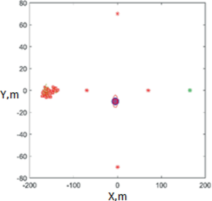

  

  Escaping from a predator with two targets

• All targets are involved: in the first iterations, the agents split into separate swarms, choosing different directions, which leads to an oscillatory process. Also, oscillation occurs when all agents have chosen the same goal. This is since the agents coordinate speed and distance among themselves Fig. 4;

• All targets are engaged, and the predator moves along the same trajectory: the agents select the same target. If the predator approaches them, the agents move away from it to a safe distance in a coordinated manner. It is worth noting that the agents only choose the direction of the temporary target. They do not have the task of reaching the temporary destination. If the predator is not in sight, the agents return to their main target, which was set before the encounter with the obstacle Fig. 6.

  Fig. 6

  

  Running away from a moving predator along a trajectory with eight targets

The units of measurement in Figs. 3, 4, 5 and 6 are in m. The horizontal axis is the X-axis, the vertical axis is the Y-axis.

The paper considers the application of the predator avoidance method in the case of such a space, which the robot cannot see now in its current position, or at the junction of two walls, behind which there is a corridor. The predator is artificially placed in the passage (blue circle in Fig. 7), or at the junction of walls in order to maneuver the agent at a greater distance: slow down before the passage to analyze the situation or with a large radius of curvature make a turn around the corner to have time to react to a possible interference.

Fig. 7

Movement of agents in the polygon in the presence of a predator

6 Movement of Agents in a Confined Space

Earlier we considered situations when agents move in unrestricted space. Agents can, oriented by the situation, go quite a long distance from the main target if the predator keeps moving in their direction.

When moving in an enclosed space, which is shown in Fig. 7, the agents perform deflection maneuvers away from obstacles. Thus, in addition to the previously considered interactions, the repulsive force from the walls is also considered. The method of potential forces is the summation of all forces of attraction to the target point and repulsion from the obstacles. It is based on realization of mobile robot movement in the field of “information forces”. The algorithms described above are based precisely on this method of correlation of arising forces in the system. When an agent moves in the polygon, the minimum distance to the walls is calculated for the method of potential forces. In Fig. 7, this is the distance between the agent (blue dot) and the intersection between the wall and the perpendicular drawn from the agent to the wall (red square). The blue circles are responsible for the areas of visibility between the agents (small circle) and the radius of visibility of the predator (large circle). The red circle represents an overview of the predator. Calculations are performed in the global coordinate system. Thus, the repulsion vector is composed of the repulsive forces of the agent from each visible wall. The predator is represented as a purple circle. Located at the intersection of two walls. Targets are represented as “*” in green.

7 Conclusion

This paper considers a model of robot swarming in the presence of a predator, designed to move autonomous agents in confined spaces with insecure areas and obstacles.

Experiments were conducted under different initial conditions and scenes. Experiments have shown that when the number of agents is greater than 10, the swarm maintains its configuration and separates in the presence of an obstacle on the way to the target.

When considering the method of fleeing from a predator, the experiment showed that the agents change their main target to a temporary one and successfully get away from dynamic obstacles. There is still work to be done on the method, as in some experiments agents split into separate groups when fleeing from a predator.

When an agent on a simulated range has an exit from a room, there is a chance that he will not have time to assess the situation if an obstacle appears in the passage. This is because the agent increases speed immediately before exiting. The proposed method of predator avoidance will allow in such situations to put “special points” in dangerous places (for example, at the corner of the corridor bend or at the exit of the room) to reduce speed in advance and bypass this area at a greater distance to assess the space.

References

Olfati-Saber R (2016) Flocking for multi-agent dynamic systems: algorithms and theory. IEEE Trans Autom Control 51(3)
Olfati-Saber R, Murray RM, Flocking with obstacle avoidance: cooperation with limited communication in mobile networks. In: 42nd IEEE international conference on decision and control, vol 2, pp 2022–2028
Helbing D, Farkas I, Vicsek T (2000) Simulating dynamical features of escape panic. Nature 407:487–490
Singh P, Tiwari R, Bhattacharya M (2010) Navigation in multi robot system using cooperative learning: a survey. In: 2016 international conference on computational techniques in information and communication technologies (ICCTICT). IEEE, New Delhi, India, 11–13 Mar 2010, pp 145–150
Reynolds CW (1987) Flocks, herds, and schools: a distributed behavioral model, in Comput. Graph. ACM SIGGRAPH’87 conference proceedings, vol 21, pp 25–34
Harary F (1969) Graph theory. Addition-Wesley
Sunehag P, Lever G, Liu S, et al. Reinforcement learning agents acquire flocking and symbiotic behaviour in simulated ecosystems. In: Artificial life conference proceedings, 2019, pp. 103–110.
Zachary Y, Hung ML (2020) Consensus, cooperative learning, and flocking for multiagent predator avoidance. Int J Adv Robot Syst 1–19. https://doi.org/10.1177/1729881420960342
Author information
Authors and Affiliations
Corresponding author
Editor information
Editors and Affiliations
Rights and permissions
Copyright information
© 2023 The Author(s), under exclusive license to Springer Nature Switzerland AG
About this chapter
Cite this chapter
Shutova, K.Y. (2023). Modeling of Unsafe Areas for Swarm Autonomous Agents. In: Vershinin, Y.A., Pashchenko, F., Olaverri-Monreal, C. (eds) Technologies for Smart Cities. Springer, Cham. https://doi.org/10.1007/978-3-031-05516-4_3
Download citation
DOI: https://doi.org/10.1007/978-3-031-05516-4_3
Published:
Publisher Name: Springer, Cham
Print ISBN: 978-3-031-05515-7
Online ISBN: 978-3-031-05516-4
eBook Packages: EngineeringEngineering (R0)