Well-Ordering Principles in Proof Theory and Reverse Mathematics

Abstract

Several theorems about the equivalence of familiar theories of reverse mathematics with certain well-ordering principles have been proved by recursion-theoretic and combinatorial methods (Friedman, Marcone, Montalbán et al.) and with far-reaching results by proof-theoretic technology (Afshari, Freund, Girard, Rathjen, Thomson, Valencia Vizcaíno, Weiermann et al.), employing deduction search trees and cut elimination theorems in infinitary logics with ordinal bounds in the latter case. At type level 1, the well-ordering principles are of the form

$$ \text { (*) } ``\text {if}\,X \text { is well-ordered then } \, f(X) \, \text { is well-ordered''} $$

where f is a standard proof-theoretic function from ordinals to ordinals (such f’s are always dilators). One aim of the paper is to present a general methodology underlying these results that enables one to construct omega-models of particular theories from $(*)$ and even $\beta$-models from the type 2 version of $(*)$. As $(*)$ is of complexity $\Pi ^1_2$ such a principle cannot characterize stronger comprehensions at the level of $\Pi ^1_1$-comprehension. This requires a higher order version of $(*)$ that employs ideas from ordinal representation systems with collapsing functions used in impredicative proof theory. The simplest one is the Bachmann construction. Relativizing the latter construction to any dilator f and asserting that this always yields a well-ordering turns out to be equivalent to $\Pi ^1_1$-comprehension. This result has been conjectured and a proof strategy adumbrated roughly 10 years ago, but a detailed proof has only been worked out in recent years.

1 Introduction

The aim to illuminate the role of the infinite in mathematics gave rise to set theory and proof theory alike. Whereas set theory takes much of the infinite for granted (e.g. full separation and powerset), proof theory strives to analyse it from a stance of potential infinity. While the objects that proof theory primarily deals with are rather concrete (e.g. theories, proofs, ordinal representation systems), it is also concerned with abstract higher type¹ properties of concrete objects (e.g. well-foundedness, preservation of well-foundedness). In ordinal analysis, the impetus is to associate an ordinal representation system $\mathcal{{OR}}$ with a theory T in such a way that the former displays the commitments to the infinite encapsulated in T. Less poetically, it entails that $\textbf{PRA}+{\textbf{TI}}_{qf}(\mathcal{{OR}})$ proves all $\Pi ^0_2$ theorems of T, however, no proper initial segment of $\mathcal{{OR}}$ suffices for that task (where $\textbf{PRA}$ refers to primitive recursive arithmetic and ${\textbf{TI}}_{qf}(\mathcal{{OR}})$ stands for quantifier-free transfinite induction along $\mathcal{{OR}}$).² The first ordinal representations were offshoots of ordinal normal forms such as Cantor’s and Veblen’s from more than a hundred years ago. Gentzen employed the Cantor normal form with base $\omega$ to provide an ordinal representation system for $\varepsilon _0$ in his last two papers [22, 23], which mark the beginning of ordinal-theoretic proof theory.

It is often stressed that ordinal representation systems are computable³ structures, which is true and allows for the treatment of their order-theoretic and algebraic aspects in very weak systems of arithmetic, but it is only one of their distinguishing features. Overstating the computability aspect tends to give the impression that their study is part of the venerable research area of computable orderings. In actual fact, the two subjects have very little in common.

There are many specific ordinal representations systems to be found in proof theory. To make the choice of these systems intelligible one would like to discern general principles involved. A particular challenge is posed by making their algebraic features explicit, i.e. those features not related to effectiveness or well-foundedness. This constitutes a crucial step towards a general theory via an axiomatic approach. As far as I’m aware, it was Feferman [11] who first initiated such a theory by isolating the property of effective relative categoricity as the fulcrum of such a characterization. Through the notion of relative categoricity, he succeeded in crystallizing the algebraic aspect of ordinal representation systems by way of relativizing them to any set of order-indiscernibles, thereby in effect scaling them up to functors on the category of linear orders with order-preserving maps as morphisms.

Ordinal representation systems understood in this relativized way give rise to well-ordering principles:

$$\text {``if}\, \mathfrak X\, \text {is a well-ordering then so is}\, \mathcal{{OR}}_{\mathfrak X}\text {''}$$

where $\mathcal{{OR}}_{\mathfrak X}$ arises from $\mathcal{{OR}}$ by letting $\mathfrak X$ play the role of the order-indiscernibles. Several theories of reverse mathematics have been shown to be equivalent to such principles involving iconic ordinal representation system from the proof-theoretic literature. From a technical point of view, the methods can be roughly divided into recursion-theoretic and combinatorial tools (Friedman, Marcone, Montalban et al.) on the one hand and proof-theoretic tools (Afshari, Freund, Girard, Rathjen, Thomson, Valencia Vizcaíno, Weiermann et al.) on the other hand, where in the latter approach the employment of deduction search trees and cut elimination theorems in infinitary logics with ordinal bounds play a central role.

This is a survey paper about these results that tries to illuminate the underlying ideas, emphasizing the proof theory side.

1.1 Reverse Mathematics

It is assumed that the reader is roughly familiar the program of Reverse Mathematics (RM) and the language and axioms of the formal system of second-order arithmetic, ${\mathbf {Z_2}}$ as, for instance, presented in the standard reference [64]. Just as a reminder, RM started out with the observation that for many mathematical theorems $\tau$, there is a weakest natural subsystem $S(\tau )$ of ${\mathbf {Z_2}}$ such that $S(\tau )$ proves $\tau$. Moreover, it has turned out that $S(\tau )$ often belongs to a small list of specific subsystems of ${\mathbf {Z_2}}$. In particular, Reverse Mathematics has singled out five subsystems of ${\mathbf {Z_2}}$, often referred to as the big five, that provide (part of) a standard scale against which the strengths of theories can often be measured:

• 1. ${\textbf{RCA}}_0$ Recursive Comprehension

• 2. ${\textbf{WKL}}_0$ Weak König’s LemmaA

• 3. ${\textbf{ACA}}_0$ Arithmetical Comprehension

• 4. ${\textbf{ATR}}_0$ Arithmetical Transfinite Recursion

• 5. $\Pi ^1_1{-}{\textbf{CA}}_0$$\Pi _1^1$-Comprehension

2 History

The principles we will be concerned with are particular $\Pi ^1_2$ statements of the form

$$\begin{aligned} {\textbf{WOP}}(f):&\;\,\,\;\;\;\forall X\,[\textrm{WO}({\mathfrak X})\rightarrow \textrm{WO}(f({\mathfrak X}))] \end{aligned}$$

(4.1)

where f is a standard proof-theoretic function from ordinals to ordinals and $\textrm{WO}({\mathfrak X})$ stands for “${\mathfrak X}$ is a well-ordering”.⁴ There are by now several examples of functions f familiar from proof theory where the statement ${\textbf{WOP}}(f)$ has turned out to be equivalent to one of the theories of reverse mathematics over a weak base theory (usually ${\textbf{RCA}}_0$). The first explicit example appears to be due to Girard [26, 5.4.1 theorem] (see also [31]). However, it is also implicit in Schütte’s proof of cut elimination for $\omega$-logic [58] and ultimately has its roots in Gentzen’s work, namely, in his first unpublished consistency proof,⁵ where he introduced the notion of a “Reduziervorschrift” [21, p. 102] for a sequent. The latter is a well-founded tree built bottom-up via “Reduktionsschritte”, starting with the given sequent and passing up from conclusions to premises until an axiom is reached.

2.1 $2^{\mathfrak X}$ and Arithmetical Comprehension

In our first example, one constructs a linear ordering $2^{\mathfrak X} = ( |2^X|,<_{_{2^X}})$ from a given linear ordering ${\mathfrak X}=(X,<_X)$, where $|2^X|$ consists of the formal sums $2^{x_1}+\ldots + 2^{x_n}$ with $x_n<_{\mathfrak X} \ldots <_{\mathfrak X}x_1$, and the ordering between two formal sums $2^{x_0}+\ldots + 2^{x_n}$, $2^{y_0}+\ldots + 2^{y_m}$ is determined as follows:

$$\begin{aligned} 2^{x_0}+\ldots + 2^{x_n}<_{2^X}2^{y_1}+\ldots + 2^{y_m}&\text { iff } \exists i\le \max (m,n)[x_i<_X y_i\,\wedge \, \forall j<i\;x_j=y_j]\\&\text { or } n<m \,\wedge \, \forall i\le n \; x_i=y_i. \end{aligned}$$

Theorem 4.1

(Girard 1987) Over ${\textbf{RCA}}_0$ the following are equivalent:

• (i) Arithmetical comprehension.

• (ii) $\forall {{\mathfrak X}}\;[\textrm{WO}({\mathfrak X})\rightarrow \textrm{WO}(2^{{\mathfrak X}})]$.

Another characterization from [26], Theorem 6.4.1, shows that arithmetical comprehension is equivalent to Gentzen’s Hauptsatz (cut elimination) for $\omega$-logic. Connecting statements of form (4.1) to cut elimination theorems for infinitary logics will be a major tool in this paper.

2.2 $\textbf{ACA}_0^+$ and $\varepsilon _{{\mathfrak X}}$

There are several more recent examples of such equivalences that have been proved by recursion-theoretic as well as proof-theoretic methods. The second example is a characterization in the same vein as (4.1) for the theory $\textbf{ACA}_0^+$ in terms of the $\xi \mapsto \varepsilon _{\xi }$ function. $\textbf{ACA}_0^+$ stands for the theory $\textbf{ACA}_0$ augmented by an axiom asserting that for any set X the $\omega$ jump in X exists. This theory is very interesting as it is currently the weakest subsystem of ${\mathbf {Z_2}}$ in which one has succeeded to prove Hindman’s Ramsey-type combinatorial theorem (asserting that finite colourings have infinite monochromatic sets closed under taking sums) and the Auslander/Ellis theorem of topological dynamics (see [64, X.3]). The source of the pertaining representation system and its relativization is the Cantor normal form.

Theorem 4.2

(Cantor, 1897) For every ordinal $\beta >0$, there exist unique ordinals $\beta _0\ge \beta _1\ge \dots \ge \beta _n$ such that

$$\begin{aligned} \beta = \omega ^{\beta _0}+\ldots +\omega ^{\beta _n}. \end{aligned}$$

(4.2)

The representation of $\beta$ in (4.2) is called the Cantor normal form. We shall write $\beta =_{_{CNF}}\omega ^{\beta _1}+\cdots +\omega ^{\beta _n}$ to convey that $\beta _0\ge \beta _1\ge \dots \ge \beta _k$.

$\varepsilon _0$ denotes the least ordinal $\alpha >0$ such that $\beta<\alpha \,\;\Rightarrow \,\;\omega ^{\beta }<\alpha$, or equivalently, the least ordinal $\alpha$ such that $\omega ^{\alpha }=\alpha$. Every $\beta <\varepsilon _0$ has a Cantor normal form with exponents $\beta _i<\beta$ and these exponents have Cantor normal forms with yet again smaller exponents, etc. As this process must terminate, ordinals $<\varepsilon _0$ can be effectively coded by natural numbers.

We state the result before introducing the functor ${\mathfrak X}\mapsto \varepsilon _{{\mathfrak X}}$.

Theorem 4.3

(Afshari, Rathjen [1]; Marcone, Montalbán [37]) Over ${\textbf{RCA}}_0$, the following are equivalent:

• (i) $\textbf{ACA}_0^+$.

• (ii) $\forall {{\mathfrak X}}\;[\textrm{WO}({\mathfrak X})\rightarrow \textrm{WO}(\varepsilon _{{\mathfrak X}})]$.

Given a linear ordering ${\mathfrak X}=\langle X,<_X\rangle$, the idea for obtaining the new linear ordering $\varepsilon _{{\mathfrak X}}$ is to create a formal $\varepsilon$-number $\varepsilon _u$ for every $u\in X$ such that if $v<_X u$ then $\varepsilon _v<_{\varepsilon _{{\mathfrak X}}}\varepsilon _u$, and in addition fill up the “spaces" between these terms with formal Cantor normal forms.

The ordering $<_{\varepsilon _{{\mathfrak X}}}$

Definition 4.4

Let ${\mathfrak X}=\langle X,<_X\rangle$ be an ordering where $X\subseteq {\mathbb N}$. $<_{\varepsilon _{{\mathfrak X}}}$ and its field $|\varepsilon _{{\mathfrak X}}|$ are inductively defined as follows:

• 1. $0\in |\varepsilon _{{\mathfrak X}}|$.

• 2. $\varepsilon _u\in |\varepsilon _{{\mathfrak X}}|$ for every $u\in X$, where $\varepsilon _u:=\langle 0,u\rangle$.

• 3. If $\alpha _1,\ldots ,\alpha _n\in |\varepsilon _{{\mathfrak X}}|$, $n>1$ and $\alpha _n\le _{\varepsilon _{{\mathfrak X}}}\ldots \le _{\varepsilon _{{\mathfrak X}}}\alpha _1$, then

  $$ \omega ^{\alpha _1}+\ldots +\omega ^{\alpha _n}\in |\varepsilon _{{\mathfrak X}}| $$

  where $\omega ^{\alpha _1}+\ldots +\omega ^{\alpha _n}:=\langle 1,\langle \alpha _1, \ldots ,\alpha _n\rangle \rangle$.

• 4. If $\alpha \in |\varepsilon _{{\mathfrak X}}|$ and $\alpha$ is not of the form $\varepsilon _u$, then $\omega ^{\alpha }\in |\varepsilon _{{\mathfrak X}}|$, where $\omega ^{\alpha }:=\langle 2,\alpha \rangle$.

• 5. $0<_{\varepsilon _{{\mathfrak X}}}\varepsilon _u$ for all $u\in X$.

• 6. $0<_{\varepsilon _{{\mathfrak X}}}\omega ^{\alpha _1}+\ldots + \omega ^{\alpha _n}$ for all $\omega ^{\alpha _1}+\ldots + \omega ^{\alpha _n}\in |\varepsilon _{{\mathfrak X}}|$.

• 7. $\varepsilon _u<_{\varepsilon _{{\mathfrak X}}}\varepsilon _v$ if $u,v\in X$ and $u<_{_X}v$.

• 8. If $\omega ^{\alpha _1}+\ldots +\omega ^{\alpha _n}\in |\varepsilon _{{\mathfrak X}}|$, $u\in X$ and $\alpha _1<_{\varepsilon _{{\mathfrak X}}}\varepsilon _u$ then $\omega ^{\alpha _1}+\ldots +\omega ^{\alpha _n} <_{\varepsilon _{{\mathfrak X}}} \varepsilon _u$.

• 9. If $\omega ^{\alpha _1}+\ldots +\omega ^{\alpha _n}\in |\varepsilon _{{\mathfrak X}}|$, $u\in X$, and $\varepsilon _u<_{\varepsilon _{{\mathfrak X}}}\alpha _1$ or $\varepsilon _u=\alpha _1$, then $\varepsilon _u<_{\varepsilon _{{\mathfrak X}}} \omega ^{\alpha _1}+\ldots +\omega ^{\alpha _n}$.

• 10. If $\omega ^{\alpha _1}+\ldots + \omega ^{\alpha _n}$ and $\omega ^{\beta _1}+\ldots + \omega ^{\beta _m}\in |\varepsilon _{{\mathfrak X}}|$, then

  

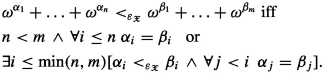
Let $\varepsilon _{\mathfrak X}= \langle |\varepsilon _{{\mathfrak X}}|,<_{\varepsilon _{{\mathfrak X}}}\rangle$.

One then proves (for instance, in $\textbf{RCA}_0$) that $\varepsilon _{\mathfrak X}$ is linear ordering. If we denote by $\mathbb{L}\mathbb{O}$ the category of linear orderings whose objects are all linear orderings and whose morphisms are the order-preserving maps between linear orderings, then ${\mathfrak X}\mapsto \varepsilon _{\mathfrak X}$ gives rise to an endofunctor of $\mathbb{L}\mathbb{O}$: For a morphism, $f:\mathfrak {X}\rightarrow \mathfrak {Y}$ define $\varepsilon (f)(t)$ for $t\in |\varepsilon _{{\mathfrak X}}|$ by replacing every expression $\varepsilon _u$ occurring in t by $\varepsilon _{f(u)}$. Then $\varepsilon (f):\varepsilon _{\mathfrak X}\rightarrow \varepsilon _{\mathfrak Y}$. Moreover, the restriction of this functor to well-orderings is a dilator in the sense of Girard [24] as it preserves pullbacks and direct limits (more about this in Sect. 4.4.2).

Ordinal Representation Systems: 1904–1909

At the beginning of the twentieth century, mathematicians were intrigued by Cantor’s continuum problem. Hardy in 1904 wanted to “construct” a subset of $\mathbb {R}$ of size $\aleph _{1}$. In [28], he gave explicit representations for all ordinals $<\omega ^2$. Hardy’s work then inspired O. Veblen, who in his paper from 1908 [69], found new normal forms for ordinals and succeeded in “naming” ordinals of an impressive chunk of the countable ordinals. In doing so, he also furnished proof theorists with the central idea for creating ordinal representation systems that were sufficient for much of their work until the middle of 1960s. His $\varphi$-function was crucial in the work of S. Feferman and K. Schütte who in the 1960s determined the limits of predicative mathematics with a notion of predicativity based on autonomous progressions of theories (cf. [10, 11, 61, 62]).

Veblen considered continuous increasing functions on ordinals. Let $\textrm{ON}$ be the class of ordinals. A (class) function $f:\textrm{ON}\rightarrow \textrm{ON}$ is said to be increasing if $\alpha <\beta$ implies $f(\alpha )<f(\beta )$ and continuous (in the order topology on $\textrm{ON}$) if

$$ f(\lim _{\xi<\lambda }\alpha _{\xi })=\lim _{\xi <\lambda }f(\alpha _{\xi }) $$

holds for every limit ordinal $\lambda$ and increasing sequence $(\alpha _{\xi })_{\xi <\lambda }$. f is called normal if it is increasing and continuous. By way of contrast, the function $\beta \mapsto \omega +\beta$ is normal, whereas $\beta \mapsto \beta +\omega$ is not since, for instance, $\lim _{\xi <\omega }(\xi +\omega )=\omega$ but $(\lim _{\xi <\omega }\xi )+\omega =\omega +\omega$.

To these normal functions Veblen applied two operations:

• (i) Derivation

• (ii) Transfinite Iteration.

The derivative $f'$ of a function $f:\textrm{ON}\rightarrow \textrm{ON}$ is the function which enumerates in increasing order the solutions of the equation

$$f( \alpha )= \alpha ,$$

also called the fixed points of f. It is a fact of set theory that if f is a normal function,

$$ \{\alpha :\,f(\alpha )=\alpha \} $$

is a proper class and $f'$ will be a normal function, too.

Using the two operations, Veblen defined a hierarchy of normal functions indexed along the ordinals.

Definition 4.5

Given a normal function $f:\textrm{ON}\rightarrow \textrm{ON}$, define a hierarchy of normal functions as follows:

• 1. $f_{0}\;=\;f ,$

• 2. $f_{\alpha +1}\;=\;{f_{\alpha }}',$

• 3.
  $$ f_{\lambda }(\xi )\; =\;\xi {{\text {th}}}\, \text {element of }\bigcap _{\alpha <\lambda } \left\{ \text {fixed points of } f_{\alpha }\right\} \phantom {AA}\text { for } \, \lambda \, \text {limit}. $$

Starting with the normal function $f(\xi )=\omega ^{\xi }$, the function $f_{\alpha }$ is usually denoted by $\varphi _{\alpha }.$

The least ordinal $\gamma >0$ closed under $\alpha ,\beta \mapsto \varphi _{\alpha }(\beta )$, i.e. the least ordinal >0 satisfying $(\forall \alpha ,\beta<\gamma )\;\varphi _{\alpha }(\beta )<\gamma$ is the famous ordinal $\Gamma _0$ that Feferman and Schütte determined to be the least ordinal “unreachable” by certain autonomous progressions of theories.

The two-place $\varphi$-function gives rise to a normal form theorem.

Theorem 4.6

($\varphi$ normal form) For every additive principal⁶ ordinal $\alpha$, there exist uniquely determined ordinals $\xi$ and $\eta$ such that $\alpha =\varphi _{\xi }(\eta )$ and $\eta <\alpha$.

Proof

See [63, Theorem 13.12] or [51, Theorem 5.27]. $\square$

The following comparison theorem encapsulates a procedure for recursively determining the order of $\varphi$-expressions, which can then be utilized to develop a representation system for the ordinals below $\Gamma _0$.

Theorem 4.7

($\varphi$-comparison)

• (i) $\varphi _{\alpha _1}(\beta _1)=\varphi _{\alpha _2}(\beta _2)$ holds iff one of the following conditions is satisfied:

  • a. $\alpha _1<\alpha _2$ and $\beta _1=\varphi _{\alpha _2}(\beta _2),$

  • b. $\alpha _1=\alpha _2$ and $\beta _1=\beta _2,$

  • c. $\alpha _2<\alpha _1$ and $\varphi _{\alpha _1}(\beta _1)=\beta _2$.

• (ii) $\varphi _{\alpha _1}(\beta _1)<\varphi _{\alpha _2}(\beta _2)$ holds iff one of the following conditions is satisfied:

  • a. $\alpha _1<\alpha _2$ and $\beta _1<\varphi _{\alpha _2}(\beta _2),$

  • b. $\alpha _1=\alpha _2$ and $\beta _1<\beta _2,$

  • c. $\alpha _2<\alpha _1$ and $\varphi _{\alpha _1}(\beta _1)<\beta _2$.

Proof

[63, Theorems 13.9, 13.10] or [51, Theorem 5.25]. $\square$

The representation system for $\Gamma _0$ can be relativized to any ordering $\mathfrak X$ by first introducing formal function symbols $\varphi _u$ for any $u\in X$ and secondly creating terms out of these using also 0 and formal addition $+$, and finally singling out the normal forms. The crucial case in defining the ordering is the following:

$$\begin{aligned} \varphi _u s<_{\varphi _{\mathfrak X}}\varphi _vt&\text { iff } u<_{_X}v\,\wedge \,s<_{\varphi _{\mathfrak X}} \varphi _v t \;\;\text { or }\\&u=v\,\wedge \,s<_{\varphi _{\mathfrak X}} t \;\;\text { or }\\&v<_{_X}u\,\wedge \,\varphi _us <_{\varphi _{\mathfrak X}} t, \end{aligned}$$

where all terms are assumed to be in normal form (for details see [37, 55]).

$\varphi _{\mathfrak X}$ induces a functor on $\mathbb{L}\mathbb{O}$ that characterizes $\textbf{ATR}_0$.

Theorem 4.8

(Friedman, unpublished; Marcone and Montalbán; Rathjen and Weiermann) Over ${\textbf{RCA}}_0$ the following are equivalent:

• 1. $\textbf{ATR}_0$

• 2. $\forall {{\mathfrak X}}\;[\textrm{WO}({\mathfrak X})\rightarrow \textrm{WO}(\varphi _{{\mathfrak X}})]$.

Friedman’s proof uses computability theory and also some proof theory. Among other things, it uses a result which states that if $P\subseteq {\mathcal P}(\omega )\times {\mathcal P}(\omega )$ is arithmetic, then there is no sequence $\{A_n\mid n\in \omega \}$ such that (a) for every n, $A_{n+1}$ is the unique set such that $P(A_n,A_{n+1})$ and (b) for every n, $A'_{n+1}\le _TA_n$.

Of the two published proofs of the foregoing theorem, A. Marcone and A. Montalbán employ tools from computability theory as their paper’s title, The Veblen function for computability theorists [37], clearly indicates. A. Weiermann and the author of this paper use purely proof-theoretic means in [55].

We would like to give the reader some insight into a proof strategy for showing theorems such as Theorems 4.3 and 4.8. However, we will be doing this by way of a different example. To state this result, it is convenient to introduce the notion of countable coded $\omega$-model.

Definition 4.9

Let T be a theory in the language of second-order arithmetic, $\mathcal {L}_2$. A countable coded $\omega$-model of T is a set $W\subseteq {\mathbb N}$, viewed as encoding the $\mathcal {L}_2$-model

$$ {\mathbb M}=({\mathbb N},{\mathcal S},\in ,+,\cdot ,0,1,<) $$

with ${\mathcal S}=\{(W)_n\mid n\in {\mathbb N}\}$ such that ${\mathbb M}\models T$ when the second-order quantifiers are interpreted as ranging over ${\mathcal S}$ and the first-order part is interpreted in the standard way (where $(W)_n=\{m\mid \langle n,m\rangle \in W\}$ with $\langle \,,\rangle$ being some primitive recursive coding function).

If T has only finitely many axioms, it is obvious how to express ${\mathbb M}\models T$ by just translating the second-order quantifiers $QX\ldots X\ldots$ in the axioms by $Qx \ldots (W)_x\ldots$. If T has infinitely many axioms,+, one needs to formalize Tarski’s truth definition for ${\mathbb M}$. This definition can be made in $\textbf{RCA}_0$ as is shown in [64], Definition II.8.3 and Definition VII.2.

We write $X\in W$ if $\exists n\;X=(W)_n$.

The notion of countable coded $\omega$-model lends itself to alternative characterizations of Theorems 4.3 and 4.8.⁷

Theorem 4.10

Over ${\textbf{RCA}}_0$ the following are equivalent:

• (i) $\forall {{\mathfrak X}}\;[\textrm{WO}({\mathfrak X})\rightarrow \textrm{WO}(\varepsilon _{{\mathfrak X}})]$ is equivalent to the statement that every set is contained in a countable coded $\omega$-model of $\textbf{ACA}_0$.

• (ii) $\forall {{\mathfrak X}}\;[\textrm{WO}({\mathfrak X})\rightarrow \textrm{WO}(\varphi {{\mathfrak X}}0)]$ is equivalent to the statement that every set is contained in a countable coded $\omega$-model of $\Delta ^1_1\text {-}{\textbf{CA}}$ (or $\Sigma ^1_1\text {-}{\textbf{DC}}$).

Proof

See [52, Corollary 1.8]. $\square$

Whereas Theorem 4.10 has been established independently by recursion-theoretic and proof-theoretic methods, there is also a result that has a very involved proof and so far has only been shown by proof theory. It connects the $\Gamma$-function with the existence of countable coded $\omega$-models of ${\textbf{ATR}}_0$. For this we need to introduce the endofunctor $\mathfrak {X}\mapsto \Gamma _{\!{\mathfrak X}}$ of $\mathbb{L}\mathbb{O}$. The linear ordering $\Gamma _{\!{\mathfrak X}}$ is created out of $\mathfrak X$ by adding formal $\Gamma$-terms $\Gamma _u$ for every $u\in X$ with the stipulation that $\Gamma _v<_{\Gamma _{\!{\mathfrak X}}}\Gamma _u$ if $v<_X u$, and in addition one fills up the “spaces” between these terms with formal sums and Veblen normal forms. The details can be found in [52, Definition 2.5].

Theorem 4.11

([52, Theorem 1.4]) Over ${\textbf{RCA}}_0$ the following are equivalent:

• (i) $\forall {{\mathfrak X}}\;[\textrm{WO}({\mathfrak X})\rightarrow \textrm{WO}(\Gamma _{\!{\mathfrak X}})]$.

• (ii) Every set is contained in a countable coded $\omega$-model of $\textbf{ATR}_0$.

The tools from proof theory employed in the above theorems involve search trees and a plethora of cut elimination techniques for infinitary logic with ordinal bounds. The search tree techniques is a starting point that all proof-theoretic proofs of the theorems of this paper have in common. It consists in producing the search or decomposition tree (in German “Stammbaum”) of a given formula. It proceeds by decomposing the formula according to its logical structure and amounts to applying logical rules backwards. This decomposition method has been employed by Schütte [59, 60] to prove the completeness theorem for $\omega$-logic. It is closely related to the method of “semantic tableaux” of Beth [6] and the tableaux of Hintikka [29]. Ultimately, the whole idea derives from Gentzen [20].

2.3 Proof Idea of (1)$\Rightarrow$(2) of Theorem 4.11

In it we shall use a simple result, namely that $\textbf{ATR}_0$ can be axiomatized via a single sentence $\Pi ^1_2$ sentence $\forall X\,C(X)$ where C(X) is $\Sigma ^1_1$ (see [64]).

Definition 4.12

Let $\textrm{L}_2$ be the language of second-order arithmetic. We assume that $\textrm{L}_2$ has relation symbols for primitive recursive relations. Formulas are generated from atomic $R(t_1,\ldots ,t_n)$ and negated atomic formulas $\lnot R(t_1,\ldots ,t_n)$ , where R is a symbol an n-ary primitive recursive relation and $t_1,\ldots ,t_n$ are numerical terms,⁸ via the logical particles $\wedge ,\vee , \exists x,\forall x,\exists X,\forall X$; so formulas are assumed to be in negation normal form.

• (a) Let $U_0,U_1,U_2,\ldots$ be an enumeration of the free set variables of $\textrm{L}_2$.

• (b) For a closed term t, let $t^{^{\mathbb N}}$ be its numerical value. We shall assume that all predicate symbols of the language $\textrm{L}_2$ are symbols for primitive recursive relations. $\textrm{L}_2$ contains predicate symbols for the primitive recursive relations of equality and inequality and possibly more (or all) primitive recursive relations. If R is a predicate symbol in ${\mathrm L}_2$ we denote by $R^{^{\mathbb N}}$ the primitive recursive relation it stands for. If $t_1,\ldots ,t_n$ are closed terms the formula $R(t_1,\ldots ,t_n)$ ($\lnot R(t_1,\ldots ,t_n)$) is said to be true if $R^{^{\mathbb N}}(t_1^{^{\mathbb N}},\ldots ,t_n^{^{\mathbb N}})$ is true (is false).

• (c) Henceforth a sequent will be a finite list of ${\mathrm L}_2$-formulas without free number variables. Sequents will be denoted by upper case Greek letters.

  Given sequents $\Gamma$ and $\Lambda$ and a formula A, we adopt the convention that $\Gamma ,A,\Lambda$ denotes the sequent resulting from extending the list $\Gamma$ by A and then extending it further by appending the list $\Lambda$.

• (i) A sequent $\Gamma$ is axiomatic if it satisfies at least one of the following conditions:

  • a. $\Gamma$ contains a true literal, i.e. a true formula of either form $R(t_1,\ldots , t_n)$ or $\lnot R(t_1,\ldots , t_n)$, where R is a predicate symbol in $\textrm{L}_2$ for a primitive recursive relation and $t_1,\ldots ,t_n$ are closed terms.

  • b. $\Gamma$ contains formulas $s\in U$ and $t\notin U$ for some set variable U and terms s, t with $s^{^{\mathbb N}}= t^{^{\mathbb N}}$.

• (iv) A sequent is reducible or a redex if it is not axiomatic and contains a formula which is not a literal.

Definition 4.13

(Deduction chains in $\omega$-logic) A deduction chain is a finite string

$$\Gamma _0;\Gamma _1;\ldots ;\Gamma _k$$

of sequents $\Gamma _i$ constructed according to the following rules:

• (i) $\Gamma _0\; = \;\emptyset$.

• (ii) $\Gamma _i$ is not axiomatic for $i<k$.

• (iii) If $i<k$ and $\Gamma _i$ is not reducible then

  $$ \Gamma _{i+1}\;=\; \Gamma _i,\lnot C(U_i). $$

• (iv) Every reducible $\Gamma _i$ with $i<k$ is of the form

  $$ \Gamma _i',E,\Gamma _i'' $$

  where E is not a literal and $\Gamma _i'$ contains only literals.

  E is said to be the redex of $\Gamma _i$.

Let $i<k$ and $\Gamma _i$ be reducible. $\Gamma _{i+1}$ is obtained from $\Gamma _i=\Gamma _i',E,\Gamma _i''$ as follows:

• 1. If $E\equiv E_0\vee E_1$ then

  $$ \Gamma _{i+1}\;=\; \Gamma _i',E_0,E_1,\Gamma _i'',\lnot C(U_i). $$

• 2. If $E\equiv E_0\wedge E_1$ then

  $$ \Gamma _{i+1}\;=\; \Gamma _i',E_j,\Gamma _i'',\lnot C(U_i) $$

  where $j=0$ or $j=1$.

• 3. If $E\equiv \exists x\,F(x)$ then

  $$ \Gamma _{i+1}\;=\; \Gamma _i',F(\bar{m}),\Gamma _i'',\lnot C(U_i),E $$

  where m is the first number such that $F(\bar{m})$ does not occur in $\Gamma _0;\ldots ;\Gamma _i$.

• 4. If $E\equiv \forall x\,F(x)$ then

  $$ \Gamma _{i+1}\;=\; \Gamma _i',F(\bar{m}),\Gamma _i'',\lnot C(U_i) $$

  for some m.

• 5. If $E\equiv \exists X\,F(X)$ then

  $$ \Gamma _{i+1}\;=\; \Gamma _i',F(U_{{m}}),\Gamma _i'',\lnot C(U_i),E $$

  where m is the first number such that $F(U_{{m}})$ does not occur in $\Gamma _0;\ldots ;\Gamma _i$.

• 6. If $E\equiv \forall X\,F(X)$ then

  $$ \Gamma _{i+1}\;=\; \Gamma _i',F(U_{{m}}),\Gamma _i'',\lnot C(U_i) $$

  where m is the first number such that $m\ne i+1$ and $U_m$ does not occur in $\Gamma _i$.

The set of deduction chains forms a tree ${\mathbb T}$ labeled with strings of sequents. We will now consider two cases.

Case I: ${\mathbb T}$ is not well-founded.

Then ${\mathbb T}$ contains an infinite path $\mathbb P$. Now define a set M via

$$\begin{aligned} (M)_i= & {} \{t^{^{\mathbb N}}\mid {t\notin U_i \, \mathrm{occurs\, in}\, {\mathbb P}}\}. \end{aligned}$$

Set ${\mathbb M}=({\mathbb N};\{(M)_i\mid i\in {\mathbb N}\},+,\cdot ,0,1,<)$.

For a formula F, let $F\in {\mathbb P}$ mean that F occurs in $\mathbb P$, i.e. $F\in \Gamma$ for some $\Gamma \in {\mathbb P}$.

Claim Under the assignment $U_i\mapsto (M)_i$ we have

$$\begin{aligned} F\in {\mathbb P}&\;\;\;\;\Rightarrow \;\;\;\;&{\mathbb M}\models \lnot F. \end{aligned}$$

The Claim implies that ${\mathbb M}$ is an $\omega$-model of $\textbf{ATR}_0$.

Case II: ${\mathbb T}$ is well-founded.

We actually want to rule this out. This is the place where the principle

$$\forall {{\mathfrak X}}\;[\textrm{WO}({\mathfrak X})\rightarrow \textrm{WO}(\Gamma _{{\mathfrak X}})]$$

in the guise of cut elimination for an infinitary proof system enters the stage. Aiming at a contradiction, suppose that ${\mathbb T}$ is a well-founded tree. Let ${\mathfrak X}_0$ be the Kleene-Brouwer ordering on ${\mathbb T}$. Then ${\mathfrak X}_0$ is a well-ordering. In a nutshell, the idea is that a well-founded ${\mathbb T}$ gives rise to a derivation of the empty sequent (contradiction) in the infinitary proof systems ${\mathcal T}^{\infty }_Q$ from [42]. This is were the really hard work lies and we have to stop here; details are in [52].

3 Towards Impredicative Theories

The proof-theoretic ordinal functions that figure in the foregoing theorems are all familiar from so-called predicative or meta-predicative proof theory. Thus far a function from genuinely impredicative proof theory is missing. The first such function that comes to mind is of the Bachmann type [4]. We will shortly turn to it.

Veblen in [69] ventured very far into the transfinite in his 1908 paper, way beyond a representation system that incorporates the $\Gamma$-function. He extended the two-place $\varphi$-function first to an arbitrary finite numbers of arguments, but then also to a transfinite numbers of arguments, with the proviso that in, for example

$$ \Phi _{f} ( \alpha _{0} , \alpha _{1} , \ldots , \alpha _{\eta } ), $$

only a finite number of the arguments $\alpha _{\nu }$ may be non-zero. In this way Veblen singled out the ordinal E(0), which is often called the big Veblen number. E(0) is the least ordinal $\delta > 0$ which cannot be named in terms of representations

$$\Phi _{\ell } ( \alpha _{0} , \alpha _{1} , \ldots , \alpha _{\eta } )$$

with $\eta < \delta$, and each $\alpha _{ \gamma } < \delta$.

3.1 The Bachmann Revelation

In a paper published in 1950, Heinz Bachmann introduced a novel idea that allowed one to “name" much larger ordinals than by the Veblen procedures. He had the amazing idea of using uncountable ordinals to keep track of diagonalizations over a hierarchies of functions. In more detail, he used the following steps:

• Define a set of ordinals ${\mathfrak B}$ closed under successor such that with each limit $\lambda \in {\mathfrak B}$ is associated an increasing sequence $\langle \lambda [\xi ]:\,\xi <\tau _{\lambda }\rangle$ of ordinals $\lambda [\xi ]\in {\mathfrak B}$ of length $\tau _{\lambda }\in {\mathfrak B}$ and $\lim _{\xi <\tau _{\lambda }}\lambda [\xi ]=\lambda$.

• Let $\Omega$ be the first uncountable ordinal. A hierarchy of functions $(\varphi ^{\!^{\mathfrak B}}_{\alpha })_{\alpha \in {\mathfrak B}}$ is then obtained as follows:

  $$\begin{aligned}&\varphi ^{\!^{\mathfrak B}}_0(\beta ) \,=\, \omega ^{\beta }\phantom {AAAA} \varphi ^{\!^{\mathfrak B}}_{\alpha +1}\, =\, \left( \varphi ^{\!^{\mathfrak B}}_{\alpha }\right) ', \end{aligned}$$

  (4.3)
  $$\begin{aligned}&\varphi ^{\!^{\mathfrak B}}_{\lambda }\;\text { enumerates }\; \bigcap _{\xi<\tau _{\lambda }}(\text {Range of }\varphi ^{\!^{\mathfrak B}}_{\lambda [\xi ]})\phantom {aaa}{\lambda \, \textrm{limit}, \tau _{\lambda }<\Omega }, \\ \nonumber&\varphi ^{\!^{\mathfrak B}}_{\lambda }\;\text { enumerates }\; \{\beta <\Omega :\,\varphi ^{\!^{\mathfrak B}}_{\lambda [\beta ]}(0)=\beta \} \phantom {aaa} {\lambda \, \textrm{limit}, \tau _{\lambda }=\Omega }. \end{aligned}$$

  (4.4)

Distilling Bachmann’s idea.

What makes Bachmann’s approach rather difficult to deal with in proof theory is the requirement to endow every limit ordinal with a fundamental sequence and referring to them when defining $\varphi _{\lambda }$, notably in the diagonalization procedure enshrined in (4.4). This layer of complication can be dispensed with though. What underpins the strength of Bachmann’s approach can be described without the bookkeeping of fundamental sequences. We start by imagining a “big" ordinal $\Omega$. What this means will become clearer as we go along, but definitely $\Omega$ should be an $\varepsilon$-number. Using ordinals $<\Omega$ and $\Omega$ itself as building blocks, one then constructs further ordinals using Cantor’s normal form, i.e. if $\alpha _1\ge \ldots \ge \alpha _n$ have already been constructed, then we build $\alpha :=\omega ^{\alpha _1}+\cdots +\omega ^{\alpha _n}$ provided that $\alpha >\alpha _1$. In this way we can build all ordinals $<\varepsilon _{\Omega +1}$, where the latter ordinal denotes the next $\varepsilon$-number after $\Omega$. Conversely, we can take any $\alpha < \varepsilon _{\Omega +1}$ apart, yielding smaller pieces as long as the exponents in its Cantor normal are smaller ordinals. This leads to the idea of support. More precisely define:

Definition 4.14

• (i) $\textsf{supp}_{\Omega }(0)=\emptyset$, $\textsf{supp}_{\Omega }(\Omega )=\emptyset$.

• (ii) $\textsf{supp}_{\Omega }(\alpha )\!=\textsf{supp}_{\Omega }(\alpha _1)\cup \cdots \cup \textsf{supp}_{\Omega }(\alpha _n)$ if $\alpha =_{CNF}\omega ^{\alpha _1}+\cdots +\omega ^{\alpha _n}> \alpha _1$.

• (iii) $\textsf{supp}_{\Omega }(\alpha )=\{\alpha \}$ if $\alpha$ is an $\varepsilon$-number $<\Omega$.

Note that $\textsf{supp}_{\Omega }(\alpha )$ is a finite set.

To define something that is equivalent to what Bachmann achieves in (4.4), the central idea is to devise an injective function

$$\vartheta :\varepsilon _{\Omega +1} \rightarrow \Omega $$

such that each $\vartheta (\alpha )$ is an $\varepsilon$-number. Think of $\vartheta$ as a collapsing, or better projection function in the sense of admissible set theory. For obvious reasons, $\vartheta$ cannot be order preserving, but the following can be realized:

$$ \alpha<\beta \,\wedge \,\textsf{supp}_{\Omega }(\alpha )<\vartheta (\beta ) \;\rightarrow \; \vartheta (\alpha )<\vartheta (\beta ). $$

With the help of $\vartheta$-function⁹ one obtains an ordinal representation system for the so-called Bachmann ordinal, also referred to as the Bachmann-Howard ordinal.¹⁰

Definition 4.15

We inductively define a set $\textsf{OT}(\vartheta )$.

• (i) $0\in \textsf{OT}(\vartheta )$ and $\Omega \in \textsf{OT}(\vartheta )$.

• (ii) If $\alpha _1,\ldots ,\alpha _n\in \textsf{OT}(\vartheta )$, $\alpha _1\ge \cdots \ge \alpha _n$, then $\omega ^{\alpha _1}+\cdots +\omega ^{\alpha _n}\in \textsf{OT}(\vartheta )$.

• (iii) If $\alpha \in \textsf{OT}(\vartheta )$ then so is $\vartheta (\alpha )$.

$(\textsf{OT}(\vartheta ),<)$ gives rise to an elementary ordinal representation system. Here < denotes the restriction to $\textsf{OT}(\vartheta )$.

The Bachmann-Howard ordinal is the order-type of $\textsf{OT}(\vartheta )\cap \Omega$.

3.2 Associating a Dilator with Bachmann

The Bachmann construction can be relativized to an arbitrary linear ordering $\mathfrak X$, as was shown in [53], giving rise to a dilator

$${\mathfrak X}\mapsto \vartheta _{\!_{\mathfrak X}}$$

and the well-ordering principle

$$\begin{aligned}&\textrm{WO}({\mathfrak X})\Rightarrow \textrm{WO}(\vartheta _{\!_{\mathfrak X}}). \end{aligned}$$

(4.5)

Definition 4.16

[53, 2.6] Again, let $\Omega$ be a “big" ordinal. Let $\mathfrak X$ be a well-ordering. With each $x\in X$ we associate a $\varepsilon$-number $\mathfrak {E}_x>\Omega$. The set of ordinals $\textsf{OT}_{\!_{\mathfrak X}}(\vartheta )$ is inductively defined as follows:

• (i) $0\in \textsf{OT}_{\!_{\mathfrak X}}(\vartheta )$, $\Omega \in \textsf{OT}_{\!_{\mathfrak X}}(\vartheta )$, and $\mathfrak {E}_x\in \textsf{OT}_{\!_{\mathfrak X}}(\vartheta )$ when $x\in X$.

• (ii) If $\alpha _1,\ldots ,\alpha _n\in \textsf{OT}_{\!_{\mathfrak X}}(\vartheta )$, $\alpha _1\ge \cdots \ge \alpha _n$, then $\omega ^{\alpha _1}+\cdots +\omega ^{\alpha _n}\in \textsf{OT}_{\!_{\mathfrak X}}(\vartheta )$.

• (iii) If $\alpha \in \textsf{OT}_{\!_{\mathfrak X}}(\vartheta )$ then so is $\vartheta _{\!_{\mathfrak X}}(\alpha )$ and $\vartheta _{\!_{\mathfrak X}}(\alpha )<\Omega$.

To explain the ordering on $\textsf{OT}_{\!_{\mathfrak X}}(\vartheta )$ one needs to extend $\textsf{supp}_{\Omega }$: Let $\textsf{supp}_{\Omega }^{\!_{\mathfrak X}}(\mathfrak {E}_x)=\emptyset$. One then sets

• 1. $\mathfrak {E}_x<\mathfrak {E}_y\,\leftrightarrow \,x<_{\mathfrak X}y$.

• 2. $\vartheta _{\!_{\mathfrak X}}(\alpha )<\vartheta _{\!_{\mathfrak X}}(\beta ) \,\leftrightarrow \,([ \alpha<\beta \,\wedge \,\textsf{supp}_{\Omega }^{\!_{\mathfrak X}}(\alpha )<\vartheta _{\!_{\mathfrak X}}(\beta )]\;\vee \;[\exists \gamma \in \textsf{supp}_{\Omega }^{\!_{\mathfrak X}}(\beta )\;\vartheta _{\!_{\mathfrak X}}(\alpha )\le \gamma ]).$

$(\textsf{OT}_{\!_{\mathfrak X}}(\vartheta ),<)$ yields an ordinal representation system elementary in $\mathfrak X$.

The principle (4.5) turns ot to be equivalent over $\textbf{RCA}_0$ to asserting that every set is contained in a countable coded $\omega$-model of the theory of Bar Induction, ${\textbf{BI}}$, whose formalization requires some preparations.

For a 2-place relation $\prec$ and an arbitrary formula F(a) of $\mathcal {L}_2$ define

• $\text {Prog}(\prec ,F):=(\forall x)[\forall y (y\prec x \rightarrow F(y))\rightarrow F(x)]$ (progressiveness),

• ${{\textbf {TI}}}(\prec ,F):= \text {Prog}(\prec ,F)\rightarrow \forall x F(x)$ (transfinite induction),

• $\text {WF}(\prec ):=\forall X{{\textbf {TI}}}(\prec ,X):=$ $\forall X(\forall x[\forall y (y\prec x \rightarrow y\in X))\rightarrow x\in X]\rightarrow \forall x[x\in X])$ (well-foundedness).

Let $\mathcal {F}$ be any collection of formulae of $\mathcal {L}_2$. For a 2-place relation $\prec$ we will write $\prec \in \mathcal {F}$, if $\prec$ is defined by a formula Q(x, y) of $\mathcal {F}$ via $x\prec y:=Q(x,y)$.

Definition 4.17

$\textrm{BI}$ denotes the bar induction scheme, i.e. all formulae of the form

$$\text {WF}(\prec )\rightarrow {{\textbf {TI}}}(\prec ,F),$$

where $\prec$ is an arithmetical relation (set parameters allowed) and F is an arbitrary formula of $\mathcal {L}_2$.

By ${\textbf{BI}}$ we shall refer to the theory ${\textbf{ACA}}_0+\textrm{BI}$.

The theorem alluded to above, due to P.F. Valencia Vizcaíno and the author, conjectured in [55, Conjecture 7.2], is the following:

Theorem 4.18

(Rathjen, Valencia Vizcaíno [53] ) Over ${\textbf{RCA}}_0$ the following are equivalent:

• 1. $\forall {{\mathfrak X}}\;[\textrm{WO}({\mathfrak X})\rightarrow \textrm{WO}(\textsf{OT}_{\!_{\mathfrak X}}(\vartheta ))]$.

• 2. Every set is contained in a countable coded $\omega$-model of $\textbf{BI}$.

4 Towards a General Theory of Ordinal Representations

We have seen several ordinal representation systems and their relativizations to an arbitrary well-ordering $\mathfrak X$. Ordinal representation systems understood in this relativized way give rise to well-ordering principles:

$$(*)\;\;\;\;\text {``if} \, \mathfrak X \;\;\text {is a well-ordering then so is}\, \mathcal{{OR}}_{\mathfrak X}\text {''}$$

where $\mathcal{{OR}}_{\mathfrak X}$ arises from $\mathcal{{OR}}$ by letting $\mathfrak X$ play the role of the order-indiscernibles. Any principle of the form $(*)$ is of syntactic complexity $\Pi ^1_2$; thus cannot characterize stronger comprehensions such as $\Pi ^1_1$-comprehension.¹¹ We are therefore led to the idea of higher order well-ordering principles. To this end we require a general theory of ordinal representation systems. A crucial step towards a general theory via an axiomatic approach was taken by Feferman in [11], who singled out the property of effective relative categoricity as central to ordinal representation systems. Through the notion of relative categoricity he succeeded in crystallizing the algebraic aspect of ordinal representation systems by way of relativizing them to any set of order-indiscernibles, thereby in effect scaling them up to functors on the category of linear orders with order-preserving maps as morphisms. Below we recall his approach in [11].

4.1 Feferman’s Relative Categoricity

Definition 4.19

Let $f_1,\ldots , f_n$ be function symbols with $f_i$ having arity $m_i$.

The set of terms $Tm(f_1,\ldots , f_n)$ is defined inductively as follows:

• (i) $\bar{0}\in Tm(f_1,\ldots , f_n)$;

• (ii) each variable $x_i$ is in $Tm(f_1,\ldots , f_n)$;

• (iii) if $t_1,\ldots ,t_{m_i}\in Tm(f_1,\ldots , f_n)$, then so also

  $$\textsf{f}_i(t_1,\ldots ,t_{m_i}).$$

Let $\textsf{Ord}$ denote the class of ordinals. Now suppose given a system of functions $F_i:\textsf{Ord}^{m_i}\rightarrow \textsf{Ord}$ (where $1\le i\le n$). By an assignment we mean any function $\sigma :\omega \rightarrow \textsf{Ord}$. With each assignment $\sigma$ and any $t\in Tm(f_1,\ldots , f_n)$ is associated an ordinal $|t|_{\sigma }$, determined as follows.

• 1. $|\bar{0}|_{\sigma } = 0$;

• 2. $|x_k|=\sigma (k)$;

• 3. $|f_i(t_1,\ldots ,t_{m_i})|_{\sigma }=F_i(|t_1|_{\sigma },\dots ,|t_{m_i}|_{\sigma })$.

The system $\vec {F}$ is said to be replete if for every ordinal $\alpha$ the closure of $\alpha$ under $\vec {F}$ is an ordinal.

An ordinal $\kappa >0$ is said to be $\vec {F}$-inaccessible if whenever $\alpha _1,\ldots ,\alpha _{m_i}<\rho$ then $F_i(\alpha _1,\ldots ,\alpha _{m_i})<\rho$ holds for all $F_i$. $\vec {F}$ is effectively relatively categorical if, roughly speaking the order relation between any two terms $s(x_1,\ldots ,x_k)$, $t(x_1,\ldots ,x_k)$ can be effectively determined from the ordering among $x_1,\ldots ,x_k$ provided that these all represent $\vec {F}$-inaccessibles. In particular for assignments $\sigma ,\tau$ into $\vec {F}$-inaccessibles it means that if

$$\forall i,j\in [1,\ldots ,n](\sigma (x_i)<\sigma (x_j)\,\leftrightarrow \,\tau (x_i)<\tau (x_j))$$

then

$$\begin{aligned}|s(x_1,\ldots ,x_k)|_{\sigma }<|t(x_1,\ldots ,x_k)|_{\sigma }&\,\leftrightarrow \,&|s(x_1,\ldots ,x_k)|_{\tau }<|t(x_1,\ldots ,x_k)|_{\tau }, \\ |t(x_1,\ldots ,x_k)|_{\sigma }<|s(x_1,\ldots ,x_k)|_{\sigma }&\,\leftrightarrow \,&|t(x_1,\ldots ,x_k)|_{\tau }<|s(x_1,\ldots ,x_k)|_{\tau },\\ |s(x_1,\ldots ,x_k)|_{\sigma }=|t(x_1,\ldots ,x_k)|_{\sigma }&\,\leftrightarrow \,&|s(x_1,\ldots ,x_k)|_{\tau }=|t(x_1,\ldots ,x_k)|_{\tau }. \end{aligned}$$

In his paper [12], with the title Hereditarily replete functionals over the ordinals, Feferman extended the foregoing notions also to finite type functionals over ordinals.

4.2 Girard’s Dilators

A general theory of ordinal representation systems was also initiated by Girard who coined the notion of dilator [24].

Let ${{\mathbb {ORD}}}$ be the category whose objects are the ordinals and whose arrows are the strictly increasing functions between ordinals. ${{\mathbb {ORD}}}$ enjoys two basic properties.

Lemma 4.20

• (i) ${\mathbb {ORD}}$ has pullbacks.

• (ii) Every ordinal is a direct limit $\varinjlim (n_p,f_{pq})_{p\subseteq q\in I}$ of a system of finite ordinals $n_p$ with I being a set of finite sets of ordinals.

Proof

(i): Let $f:\alpha \rightarrow \gamma$ and $g:\beta \rightarrow \gamma$ be in ${\mathbb {ORD}}$. One easily checks that any $h:\delta \rightarrow \gamma$ such that

$$\begin{aligned} {\textrm{ran}}(h)= & {} {\textrm{ran}}(f)\cap {\textrm{ran}}(g)\end{aligned}$$

(4.6)

is a pullback of $f:\alpha \rightarrow \gamma$ and $g:\beta \rightarrow \gamma$. Note that $h:\delta \rightarrow \gamma$ is uniquely determined by (4.6) and that such an h always exists: Let $\delta$ be the Mostowski collapse of ${\textrm{ran}}(f)\cap {\textrm{ran}}(g)$, $\textsf{clpse}_{{\textrm{ran}}(f)\cap {\textrm{ran}}(g)}$ be the pertaining collapsing function, and h be the inverse of the collapsing function.

(ii): Fix an ordinal $\alpha$. Let I be the collection of finite subsets of $\alpha$. I is ordered by the inclusion relation, which is also directed, i.e. for $s,t\in I$ there exists $q\in I$ such that $s\subseteq q$ and $t\subseteq q$. Let $s\in I$. Then $s=\{\alpha _0,\ldots ,\alpha _{n-1}\}$ for uniquely determined ordinals $\alpha _0<\ldots <\alpha _{n-1}$. Define $n_s:=n$ and $f_s:n_s\rightarrow s$ by $f_s(i)=\alpha _i$. By design, $f_s$ is an order-preserving bijection between $n_s$ and s. For $p\subseteq q\in I$ define $f_{pq}:n_p\rightarrow n_q$ by $f_{pq}:= (f_q)^{-1}\circ f_p$. Thus, $f_{pp}$ is the identity on $n_p$, and if $p\subseteq q\subseteq r$, one has $f_{pr}= f_{qr}\circ f_{pq}$. As a result,

$$\qquad \qquad \qquad \qquad \qquad \qquad \alpha =\varinjlim (n_p,f_{pq})_{p\subseteq q\in I}. \qquad \qquad \qquad \qquad \qquad \qquad \qquad \qquad \qquad \square $$

Of special interest are the endofunctors of this category that can be characterized by the two foregoing notions.

Definition 4.21

A dilator is an endofunctor of the category ${{\mathbb {ORD}}}$ preserving direct limits and pullbacks.

Dilators can be characterized in straightforward way.

Lemma 4.22

For a functor $F:{\mathbb {ORD}}\rightarrow {\mathbb {ORD}}$, the following are equivalent:

• (i) F is a dilator.

• (ii) F has the following two properties:

  • a. Whenever $f:\alpha \rightarrow \gamma$, $g:\beta \rightarrow \gamma$, $h:\delta \rightarrow \gamma$, then

    $$\begin{aligned} {\textrm{ran}}(h)={\textrm{ran}}(f)\cap {\textrm{ran}}(g)\Rightarrow & {} {\textrm{ran}}(F(h))={\textrm{ran}}(F(f))\cap {\textrm{ran}}(F(g))\nonumber \\ \end{aligned}$$

    (4.7)

  • b. For every ordinal $\alpha$ and $\eta <F(\alpha )$ there exists a finite ordinal n and strictly increasing function $f:n \rightarrow \alpha$ such that $\eta \in {\textrm{ran}}(F(f))$.

Proof

It follows from the proof of Lemma 4.20(i) that preservation of pullbacks and condition (ii)(a) are equivalent. It remains to show that in ${\mathbb {ORD}}$ preservation of direct limits and condition (ii)(b) amount to the same. This can be gleaned from the proof of Lemma 4.20(ii), however, as the details are not relevant for this paper, we just refer to [24] for the details. $\square$

There is an easy but important consequence of the above, i.e. of Lemma 4.20(ii).

Lemma 4.23

A dilator is completely determined by its behaviour on the subcategory of finite ordinals and morphisms between them, ${\mathbb {ORD}}_{\omega }$.

At this point, it is perhaps not immediately gleanable what the connection between ordinal representation systems and dilators might be. This is what we turn to next.

Denotation systems and dilators

Girard (cf. [24, 25, 27]) provided an alternative account of dilators that assimilates them more closely to ordinal representation systems and in particular to Feferman’s notion of relative categoricity.

Definition 4.24

Let $\textrm{ON}$ be the class of ordinals and $F:\textrm{ON}\rightarrow \textrm{ON}$. A denotation-system for F is a class $\mathcal D$ of ordinal denotations of the form

$$(c;\alpha _0,\ldots ,\alpha _{n-1};\alpha )$$

together with an assignment $D:{\mathcal D}\rightarrow \textrm{ON}$ such that the following hold:

• 1. If $(c;\alpha _0,\ldots ,\alpha _{n-1};\alpha )$ is in $\mathcal D$, then $\alpha _0<\ldots<\alpha _{n-1}<\alpha$ and $D(c;\alpha _0,\ldots ,\alpha _{n-1};\alpha )< F(\alpha )$.

• 2. Every $\beta <F(\alpha )$ has a unique denotation $(c;\alpha _0,\ldots ,\alpha _{n-1};\alpha )$ in $\mathcal D$, i.e.

  $\beta =D(c;\alpha _0,\ldots ,\alpha _{n-1};\alpha )$.

• 3. If $(c;\alpha _0,\ldots ,\alpha _{n-1};\alpha )$ is a denotation and $\gamma _0<\ldots<\gamma _{n-1}<\gamma$, then $(c;\gamma _0,\ldots ,\gamma _{n-1};\gamma )$ is a denotation.

• 4. If $D(c;\alpha _0,\ldots ,\alpha _{n-1};\alpha )\le D(d;\alpha _0',\ldots ,\alpha _{m-1}';\alpha )$, $\gamma _0<\ldots<\gamma _{n-1}<\gamma$, $\gamma _0'<\ldots<\gamma _{m-1}'<\gamma$, and for all $i<n$ and $j<m$,

  $$\alpha _i\le \alpha _j'\Leftrightarrow \gamma _i\le \gamma _j' \;\;\text { and }\;\; \alpha _i\ge \alpha _j'\Leftrightarrow \gamma _i\ge \gamma _j'$$

  then

  $$D(c;\gamma _0,\ldots ,\gamma _{n-1};\gamma )\le D(d;\gamma _0',\ldots ,\gamma _{m-1}';\gamma ).$$

In a denotation $(c;\alpha _0,\ldots ,\alpha _{n-1};\alpha )$, c is called the index, $\alpha$ is the parameter and $\alpha _0,\ldots ,\alpha _{n-1}$ are the coefficients of the denotation. If $\beta =D(c;\alpha _0,\ldots ,\alpha _{n-1};\alpha )$, the index c represents some ‘algebraic’ way of describing $\beta$ in terms of the ordinals $\alpha _0,\ldots ,\alpha _{n-1},\alpha$.

Lemma 4.25

Every denotation system D induces a dilator $F_{\!_D}$ by letting $F_{\!_D}(\alpha )$ be the least ordinal $\eta$ that does not have a denotation of the form $D(c;\alpha _0,\ldots ,\alpha _{n-1};\alpha )$, and for any arrow $f:\alpha \rightarrow \delta$ of the category ${\mathbb {ORD}}$ letting

$$F_{\!_D}(f):F_{\!_D}(\alpha )\rightarrow F_{\!_D}(\delta )$$

be defined by

$$F_{\!_D}(f)(D(c;\alpha _0,\ldots ,\alpha _{n-1};\alpha ))\;:=\; D(c;f(\alpha _0),\ldots ,f(\alpha _{n-1});\delta ).$$

The converse is also true.

Lemma 4.26

To every dilator F one can assign a denotation system $D_{\!_F}$ such that $\beta <F(\alpha )$ is denoted by

$$(\gamma ;\alpha _0,\ldots ,\alpha _{n-1};\alpha )$$

where n is the least finite ordinal such that there exists a morphism $f:n\rightarrow \alpha$ with $\beta \in {\textrm{ran}}(F(f))$. Moreover, $\gamma <F(n)$ is uniquely determined by $F(f)(\gamma )=\beta$, and $\alpha _0=f(0),\ldots ,\alpha _{n-1}=f(n-1)$.

Proof

F being a dilator, we know that such an f exists. f is also uniquely determined since n is chosen minimal: for if $g:n\rightarrow \alpha$ also satisfied $\beta \in {\textrm{ran}}(F(g))$, then their joint pullback $h:m\rightarrow \alpha$ would satisfy $\beta \in {\textrm{ran}}(h)$ as well, so that $n=m$ and ${\textrm{ran}}(h)={\textrm{ran}}(f)={\textrm{ran}}(g)$, meaning $f=g$. $\square$

5 Higher Order Well-Ordering Principles

We already noted that a statement of the form ${\textbf{WOP}}(f)$ is $\Pi ^1_2$ and therefore cannot be equivalent to a theory whose axioms have an essentially higher complexity, like for instance $\Pi ^1_1$-comprehension. The idea thus is that to get equivalences one has to climb up in the type structure. Given a functor

$$F:({\mathbb{L}\mathbb{O}}\rightarrow {\mathbb{L}\mathbb{O}})\rightarrow ({\mathbb{L}\mathbb{O}}\rightarrow {\mathbb{L}\mathbb{O}}),$$

where ${\mathbb{L}\mathbb{O}}$ is the class of linear orderings, we consider the statement¹²:

$${\mathbb {HWOP}}(F):\phantom {AAA}\forall f\in ({\mathbb{L}\mathbb{O}}\rightarrow {\mathbb{L}\mathbb{O}})\;[{\textbf{WOP}}(f)\rightarrow {\textbf{WOP}}(F(f))].$$

There is also a variant of ${\mathbb {HWOP}}(F)$ which should basically encapsulate the same “power”. Given a functor

$$G:({\mathbb{L}\mathbb{O}}\rightarrow {\mathbb{L}\mathbb{O}})\rightarrow {\mathbb{L}\mathbb{O}}$$

consider the statement:

$${\mathbb {HWOP}}_1(G):\phantom {AAA}\forall f\in ({\mathbb{L}\mathbb{O}}\rightarrow {\mathbb{L}\mathbb{O}})\;[{\textbf{WOP}}(f)\rightarrow \textrm{WO}(G(f))].$$

It was conjectured in [38] that a principle of the form ${\mathbb {HWOP}}(F)$ might be equivalent to $\Pi ^1_1$-comprehension. In [56] is was claimed that for a specific functor ${\mathcal B}:({\mathbb{L}\mathbb{O}}\rightarrow {\mathbb{L}\mathbb{O}})\rightarrow {\mathbb{L}\mathbb{O}}$, ${\mathbb {HWOP}}_1({\mathcal B})$ is equivalent to $\Pi ^1_1$-comprehension. ${\mathcal B}$ is a functor that takes an arbitrary dilator F as input and returns an ordinal representation system; this amounts to combining the Bachmann procedure with the closure under F. [56] also adumbrated the steps and a proof strategy for this result.

5.1 Bachmann Meets a Dilator

The idea to combine the Bachmann construction with an arbitrary dilator one finds in [38, 56]. The details were worked out in Anton Freund’s thesis [13].¹³

Definition 4.27

Again, let $\Omega$ be a “big” ordinal. Let $\mathcal D$ be a system of denotations.

• (i) $0\in \textsf{OT}_{\!_{\mathcal D}}(\vartheta )$, $\Omega \in \textsf{OT}_{\!_{\mathcal D}}(\vartheta )$.

• (ii) If $\alpha _1,\ldots ,\alpha _n\in \textsf{OT}_{\!_{\mathcal D}}(\vartheta )$, $\alpha _1\ge \cdots \ge \alpha _n$, then $\omega ^{\alpha _1}+\cdots +\omega ^{\alpha _n}\in \textsf{OT}_{\!_{\mathcal D}}(\vartheta )$.

• (iii) If $\alpha \in \textsf{OT}_{\!_{\mathcal D}}(\vartheta )$ then so is $\vartheta _{\!_{\mathcal D}}(\alpha )$ and $\vartheta _{\!_{\mathcal D}}(\alpha )<\Omega$.

• (iv) If $\alpha _0,\ldots ,\alpha _{n-1}\in \textsf{OT}_{\!_{\mathcal D}}(\vartheta )$, $\alpha _0<\cdots<\alpha _{n-1}<\Omega$, and $\sigma =(c;0,\ldots ,n-1;n)\in \mathcal {D}$, then

  $$\mathfrak {E}^{\sigma }_{\alpha _0,\ldots ,\alpha _{n-1}}\in \textsf{OT}_{\!_{\mathcal D}}(\vartheta )\text { and }\Omega <\mathfrak {E}^{\sigma }_{\alpha _0,\ldots ,\alpha _{n-1}}.$$

To explain the ordering on $\textsf{OT}_{\!_{\mathcal D}}(\vartheta )$ one needs to extend $\textsf{supp}_{\Omega }$: Let

$$\textsf{supp}_{\Omega }^{\!_{\mathcal D}}(\mathfrak {E}^{\sigma }_{\alpha _0,\ldots ,\alpha _{n-1}})=\{\alpha _0,\ldots ,\alpha _{n-1}\}.$$

The ordering between $\vartheta _{\!_{\mathcal D}}$-terms is defined as before:

$$ \vartheta _{\!_{\mathcal D}}(\alpha )<\vartheta _{\!_{\mathcal D}}(\beta ) \,\leftrightarrow \,([\alpha<\beta \,\wedge \,\textsf{supp}_{\Omega }^{\!_{\mathcal D}}(\alpha )<\vartheta _{\!_{\mathcal D}}(\beta )]\;\vee \;[\exists \gamma \in \textsf{supp}_{\Omega }^{\!_{\mathcal D}}(\beta )\, \vartheta _{\!_{\mathcal D}}(\alpha )\le \gamma ]).$$

How do we compare terms of the form $\mathfrak {E}^{\sigma }_{\alpha _0,\ldots ,\alpha _{n-1}}$ and $\mathfrak {E}^{\tau }_{\beta _0,\ldots ,\beta _{m-1}}$? To this end let $\sigma =(c;0,\ldots ,n-1;n)$ and $\tau =(e;0,\ldots ,m-1;m)$; also let k be the number of elements of $\{\alpha _0,\ldots ,\alpha _{n-1},\beta _0,\ldots ,\beta _{m-1}\}$. In a first step, define $f:n\rightarrow k$ and $g:m\rightarrow k$ such that

$$\begin{aligned} f(i)< g(j)&\,\leftrightarrow \,&\alpha _i<\beta _j , \\ f(i)=g(j)&\,\leftrightarrow \,&\alpha _i=\beta _j.\end{aligned}$$

Then

$$\mathfrak {E}^{\sigma }_{\alpha _0,\ldots ,\alpha _{n-1}} \;<\;\mathfrak {E}^{\tau }_{\beta _0,\ldots ,\beta _{m-1}}$$

if and only if

$$D(c;f(0),\ldots ,f(n-1);k) \;<\;D(e;g(0),\ldots ,g(m-1);k).$$

It is rather instructive to see why $\textsf{OT}_{\!_{\mathcal D}}(\vartheta )$ is a well-ordering.We shall prove that with the help of strong comprehension.

Theorem 4.28

($\Pi ^1_1\text {-}\textbf{CA}_0$) For every dilator $\mathcal D$, $(\textsf{OT}_{\!_{\mathcal D}}(\vartheta ),<)$ is a well-ordering.

Proof

Let I be the well-founded part of $\textsf{OT}_{\!_{\mathcal D}}(\vartheta )\cap \Omega :=\{\alpha \in \textsf{OT}_{\!_{\mathcal D}}(\vartheta )\mid \alpha <\Omega \}$. $\Pi ^1_1$-comprehension ensures that I is a set. Then ${\mathfrak I}:=(I,<\restriction I\times I)$ is a well-ordering. Now let

$${M}\,:=\,\{\beta \in \textsf{OT}_{\!_{\mathcal D}}(\vartheta )\mid \textsf{supp}_{\Omega }^{\!_{\mathcal D}}(\beta )\subseteq I\}\;\text { and }\;\mathfrak {M}\,:=\, (M,<\restriction M\times M).$$

We claim that $\mathfrak {M}$ is a well-ordering, too. To see this, note that the set of terms of the form $\mathfrak {E}^{\sigma }_{\alpha _0,\ldots ,\alpha _{n-1}}$ with $\alpha _0,\ldots ,\alpha _{n-1}\in I$ is well-ordered as they are in one-one and order preserving correspondence with the denotations $D(c;\alpha _0,\ldots ,\alpha _{n-1};\mathfrak {I})$ where $\sigma =(c;0,\ldots ,n-1;n)$. Now, M is obtained from I by adding the latter terms as well as $\Omega$, and then closing off under $+$ and $\xi \mapsto \omega ^{\xi }$ (or more precisely, Cantor normal forms). It is known from Gentzen’s [23] that this last step preserves well-orderedness.¹⁴

Thus, if we can show that $\textsf{OT}_{\!_{\mathcal D}}(\vartheta )$ is the same as $\mathfrak M$ we are done. For this it is enough to establish closure of M under $\vartheta _{\!_{\mathcal D}}$.

$$\mathsf {Claim:}\;\;\; \forall \alpha \in M\;\vartheta _{\!_{\mathcal D}}(\alpha )\in M.$$

The Claim is proved by induction on $\alpha$. So assume $\alpha \in M$ and

$$(*)\;\;\;\forall \beta \in M\;[\beta <\alpha \rightarrow \vartheta _{\!_{\mathcal D}}(\beta )\in I].$$

To be able to conclude that $\vartheta _{\!_{\mathcal D}}(\alpha )\in I$, it suffices to show that $\delta \in I$ holds for all $\delta < \vartheta _{\!_{\mathcal D}}(\beta )$. We establish this via a subsidiary induction on the syntactic complexity of $\delta$ (so this is in effect an induction on naturals). If $\delta =0$ this is immediate, and if $\delta =\omega ^{\delta _1}+\ldots +\omega ^{\delta _n}$ with $\delta >\delta _1\ge \ldots \ge \delta _n$ this follows from the subsidiary induction hypothesis and the fact that I is closed under $+$ and $\xi \mapsto \omega ^{\xi }$.

This leaves the case that $\delta =\vartheta _{\!_{\mathcal D}}(\rho )$ for some $\rho$. Since $\vartheta _{\!_{\mathcal D}}(\rho )< \vartheta _{\!_{\mathcal D}}(\alpha )$ there are two subcases to consider.

Case 1: $\rho <\alpha$ and $\textsf{supp}_{\Omega }^{\!_{\mathcal D}}(\rho )<\vartheta _{\!_{\mathcal D}}(\alpha )$. By the subsidiary induction hypothesis, $\textsf{supp}_{\Omega }^{\!_{\mathcal D}}(\rho )\subseteq I$ as the syntactic complexity of terms in $\textsf{supp}_{\Omega }^{\!_{\mathcal D}}(\rho )$ is not bigger than that of $\rho$ and thus smaller than that of $\delta$. Therefore, $\rho \in M$, and since $\rho <\alpha$ it follows from $(*)$ that $\delta =\vartheta _{\!_{\mathcal D}}(\rho )\in I$.

Case 2: There exists $\xi \in \textsf{supp}_{\Omega }^{\!_{\mathcal D}}(\alpha )$ such that $\delta \le \xi$. $\alpha \in M$ entails that $\xi \in I$, and thus $\delta \in I$. $\square$

Theorem 4.29

The following are equivalent over $\textbf{RCA}_0$:

• (i) $\Pi ^1_1$-comprehension.

• (ii) For every denotation system $\mathcal D$, $\textsf{OT}_{\!_{\mathcal D}}(\vartheta )$ is a well-ordering.

A proof of this result was adumbrated in [56] while the first detailed proof was given in Anton Freund’s thesis [13] and in his papers [14,15,16]. Below, however, we will be presenting another proof, partly going back to [56], since the purpose here is to convey the intuitions behind the result to the reader and present them without employing category-theoretic terminology.

The direction (i)$\Rightarrow$(ii) of Theorem 4.29 is taken care of by Theorem 4.28. Next, we will be concerned with giving a proof sketch for the direction $(*)$ (ii)$\Rightarrow$(i). For $(*)$ it is enough to show that every set $\bar{Q}\subseteq \mathbb {N}$ is contained in a countable coded model ${\mathfrak M}=(M,E)$ of Kripke-Platek set theory (with Infinity), where the interpretation E of the elementhood relation is well-founded. This is so because a $\Pi ^1_1$-definable class of naturals, $\{n\in \mathbb {N}\mid F(n,\bar{Q})\}$, with second-order parameter $\bar{Q}$ is $\Sigma _1$-definable over $\mathfrak M$ (see [5, IV.3.1]), and therefore a set in the background theory. Important techniques include Schütte’s method of search trees [59] for $\omega$-logic but adjusted to $\alpha$-logic for any ordinal (or rather well-ordering) $\alpha$ and proof calculi similar to the one used for the ordinal analysis of Kripke-Platek set theory (originally due to Jäger [32, 33]). It is not necessary, though, to use the machinery for the ordinal analysis of $\textbf{KP}$. Instead, one can also directly employ the older techniques from ordinal analyses of the formal theory of non-iterated arithmetic inductive definitions as presented in [39, 40]. Technically, though, the easiest approach appears to be to work with an extension of Peano arithmetic with inductive definitions and an extra sort of ordinals to express the stages of an inductive definition as in Jäger’s $\textbf{PA}_{\Omega }$ from [34].

Definition 4.30

In what follows, we fix a set $\bar{Q}\subseteq \mathbb {N}$ and a well-ordering $\mathfrak {X}=(X,<_X)$ with $X\subseteq \mathbb {N}$. Let $L_1$ be the first-order language of arithmetic with number variables $x, y, z, \ldots$ (possibly with subscripts), the constant 0, as well as function and relation symbols for all primitive recursive functions and relations, and a unary predicate symbol Q. Let $L_1(P)$ be the extension of $L_1$ by a further “fresh” unary relation symbol P. The atomic formulas of $L_1(P)$ are of the form Q(t), P(t) and $R(s_1,\ldots ,s_k)$, where $t,s_1,\ldots ,s_k$ are terms and R is a relation symbol for a primitive recursive k-ary relation. The literals of $L_1(P)$ are the atomic formulas and their negations $\lnot Q(t)$, $\lnot P(t)$ and $\lnot R(s_1,\ldots ,s_k)$. The formulas of $L_1(P)$ are then generated from the literals via the logical connectives $\wedge ,\vee$ and the quantifiers $\forall x$ and $\exists x$. Note that the formulas are in negation normal form. As per usual, negation is a defined operation, using deletion of double negations and de Morgan’s laws. A formula is said to be P-positive if it contains no occurrences of the form $\lnot P(t)$. A P-positive formula in which at most the variable x occurs free will be called an inductive operator form; expressions A(P, x) are meant to range over such forms.

$L_1$ will be further extended to a new language $L_{_\mathfrak {X}}$ by adding a new sort of ordinal variables $\alpha ,\beta ,\gamma ,\ldots$ (possibly with subscripts), a new binary relation symbol < for the less relation on the ordinals¹⁵ and a binary relation symbol $P_A$ for each inductive operator form A(P, x).¹⁶ For each element u of the well-ordering $\mathfrak {X}$ we also introduce an ordinal constant $\alpha _u$ into the language $L_{_\mathfrak {X}}$. Ordinal constants inherit an ordering from $\mathfrak X$, namely $\alpha _u$ is considered to be smaller than $\alpha _v$ if $u<_Xv$. In future, when we talk about the least ordinal constant satisfying a certain condition we are referring to that ordering.

Since subscripts are often a nuisance to humans, we will use overlined ordinal variables, i.e. $\bar{\alpha },\bar{\beta },\ldots$, as metavariables for these constants.

The number terms $s, t, \ldots$ of $L_{_\mathfrak {X}}$ are the number terms of $L_1$; the ordinal terms of $L_{_\mathfrak {X}}$ are the ordinal variables and constants. The formulas of $L_{_\mathfrak {X}}$ are inductively generated as follows:

• 1. If R is a k-ary relation symbol of $L_1$ and $s_1,\ldots ,s_k$ are number terms, then $R(s_1,\ldots ,s_k)$ is an atomic formula of $L_{_\mathfrak {X}}$.

• 2. $\mathfrak {a}<\mathfrak {b}$, $\mathfrak {a}=\mathfrak {b}$ and $P_A(s,\mathfrak {a})$ are atomic formulas of $L_{_\mathfrak {X}}$ whenever $\mathfrak {a}$ and $\mathfrak {b}$ are ordinal terms and s is a number term.

• 3. Negations of atomic formulas of $L_{_\mathfrak {X}}$ are formulas of $L_{_\mathfrak {X}}$. The latter together with the atomic formulas make up the literals of $L_{_\mathfrak {X}}$.

• 4. If B, C are formulas of $L_{_\mathfrak {X}}$, then so are $B\wedge C$ and $B\vee C$.

• 5. If F(x) is a formula of $L_{_\mathfrak {X}}$, then so are $\exists xF(x)$ and $\forall xF(x)$.

• 6. If $G(\alpha )$ is a formula of $L_{_\mathfrak {X}}$, then so are $\exists \alpha G(\alpha )$ and $\forall \alpha F(\alpha )$.

• 7. If $G(\alpha )$ is a formula of $L_{_\mathfrak {X}}$ and $\mathfrak {b}$ is an ordinal term, then so are $(\exists \alpha <\mathfrak {b})\, G(\alpha )$ and $(\forall \alpha <\mathfrak {b})\, F(\alpha )$.

As per usual, $B\rightarrow C$ is an abbreviation for $\lnot B\,\vee \,C$ (with $\lnot$ being the obvious defined operation of negation), and $B\leftrightarrow C$ abbreviates $(B\rightarrow C)\,\wedge \,(C\rightarrow B)$.

In future, we write $P^{\mathfrak {a}}_A(s)$ for $P_A(s,\mathfrak {a})$. We also write $P^{<\mathfrak {a}}_A(s)$ for $(\exists \beta <\mathfrak {a})\,P^{\beta }_A(s)$ and $P_A(s)$ for $\exists \alpha \,P^{\alpha }_A(s)$.

Definition 4.31

The axioms of $\textbf{PA}_{_{\mathfrak X}}$ fall into several groups:

• 1. True literals: These are of three forms.

  • a. Let R be a symbol for a k-ary primitive recursive relation and $s_1,\ldots ,s_k$ are closed number terms. $R(s_1,\ldots ,s_k)$ is a true literal if $\mathcal {R}(s^{\mathbb N}_1,\ldots , s^{\mathbb N}_1)$ is true in the naturals, where $\mathcal {R}$ denotes the predicate pertaining to R and $s^{\mathbb {N}}_i$ denotes the value of the closed number term $s_i$ in the standard interpretation; if $R(s_1,\ldots ,s_k)$ is false under the standard interpretation, then $\lnot R(s_1,\ldots ,s_k)$ is a true literal.

  • b. Q(s) is a true literal if $s^{\mathbb {N}}_i\in \bar{Q}$, and $\lnot Q(t)$ is a true literal if $t^{\mathbb {N}}_i\notin \bar{Q}$, where s, t are closed numeral terms.

  • c. Let $\alpha _u,\alpha _v$ are ordinal constants with $u,v\in \mathfrak {X}$. $\alpha _u<\alpha _v$ is a true literal if $u<_Xv$, and otherwise $\lnot \,\alpha _u<\alpha _v$ is a true literal. $\alpha _u=\alpha _u$ is a true literal whereas $\lnot \alpha _u=\alpha _v$ is a true literal if $u\ne v$.

• 2. Stage axioms: These are all sentences of the form $\forall \alpha \,\forall x\,[A(P_A^{<\alpha },x)\rightarrow P_A^{\alpha }(x)]$.

• 3. Reflection: These are all sentences of the form $\forall x\,[A(P_A,x)\rightarrow \exists \alpha \,P^{\alpha }_A(s)]$.

• 4. Let $A_0,A_1,\ldots$ be a fixed enumeration of all stage and reflection axioms. Note that all of these are closed formulas (sentences) and that none of them contains any ordinal constants.

5.2 Deduction Chains in $\textbf{PA}_{_{\mathfrak X}}$

Sequents are finite lists of sentences of $L_{_\mathfrak {X}}$; they will be notated by upper case Greek letters.¹⁷

Definition 4.32

• (i) A sequent $\Gamma$ is axiomatic if it contains a true literal.¹⁸

• (ii) A sequent is reducible or a redex if it is not axiomatic and contains a formula which is not a literal.

Definition 4.33

A $\textbf{PA}_{_{\mathfrak X}}$-deduction chain is a finite string

$$\Gamma _0;\Gamma _1;\ldots ;\Gamma _k$$

of sequents $\Gamma _i$ constructed according to the following rules:

• (i) $\Gamma _0\; = \;\emptyset$.

• (ii) $\Gamma _i$ is not axiomatic for $i<k$.

• (iii) If $i<k$ and $\Gamma _i$ is not reducible then

  $$\Gamma _{i+1}\;=\; \Gamma _i,\lnot A_i$$

  where $A_i$ is the i-th formula in the list from Definition 4.31(4).

• (iv) Every reducible $\Gamma _i$ with $i<k$ is of the form

  $$\Gamma _i',E,\Gamma _i''$$

  where E is not a literal and $\Gamma _i'$ contains only literals. E is said to be the redex of $\Gamma _i$.

  Let $i<k$ and $\Gamma _i$ be reducible. $\Gamma _{i+1}$ is obtained from $\Gamma _i=\Gamma _i',E,\Gamma _i''$ as follows:

  • a. If $E\equiv E_0\vee E_1$ then

    $$\Gamma _{i+1}\;=\; \Gamma _i',E_0,E_1,\Gamma _i'',\lnot A_i.$$

  • b. If $E\equiv E_0\wedge E_1$ then

    $$\Gamma _{i+1}\;=\; \Gamma _i',E_j,\Gamma _i'',\lnot A_i$$

    where $j=0$ or $j=1$.

  • c. If $E\equiv \exists x\in {\mathbb N}\,F(x)$ then

    $$\Gamma _{i+1}\;=\; \Gamma _i',F(\bar{m}),\Gamma _i'',\lnot A_i,E$$

    where m is the first number such that $F(\bar{m})$ does not occur in $\Gamma _0;\ldots ;\Gamma _i$.¹⁹

  • d. If $E\equiv \forall x\in {\mathbb N}\,F(x)$ then

    $$\Gamma _{i+1}\;=\; \Gamma _i',F(\bar{m}),\Gamma _i'',\lnot A_i$$

    for some m.

  • e. If $E\equiv \exists \xi \,F(\xi )$ then

    $$\Gamma _{i+1}\;=\; \Gamma _i',F(\bar{\delta }),\Gamma _i'',\lnot A_i,E$$

    where the ordinal constant $\bar{\delta }$ is picked as follows. If there occurs an ordinal constant $\bar{\gamma }$ in $\Gamma _0;\ldots ;\Gamma _i$ such that $F(\bar{\gamma })$ does not occur in $\Gamma _0;\ldots ;\Gamma _i$ then let $\bar{\delta }$ be the least such (with leastness understood in the sense of $\mathfrak X$). If, however, for all ordinal constants $\bar{\gamma }$ in $\Gamma _0;\ldots ;\Gamma _i$ the formula $F(\bar{\gamma })$ already occurs in $\Gamma _0;\ldots ;\Gamma _i$, then $\bar{\delta }$ can be any ordinal constant.²⁰

  • f. If $E\equiv \forall \xi \,F(\xi )$ then

    $$\Gamma _{i+1}\;=\; \Gamma _i',F(\bar{\delta }),\Gamma _i'',\lnot A_i$$

    where $\bar{\delta }$ is any ordinal constant.

  • g. If $E\equiv (\exists \xi <\bar{\alpha })\,F(\xi )$. then

    $$\Gamma _{i+1}\;=\; \Gamma _i',\bar{\delta }<\bar{\alpha }\,\wedge \,F(\bar{\delta }),\Gamma _i'',\lnot A_i,E$$

    where the ordinal constant $\bar{\delta }$ is picked as follows: If there occurs an ordinal constant $\bar{\gamma }$ in $\Gamma _0;\ldots ;\Gamma _i$ such that $\bar{\gamma }<\bar{\alpha }$ is true and $F(\bar{\gamma })$ does not occur in $\Gamma _0;\ldots ;\Gamma _i$, let $\bar{\delta }$ be the least such. If, however, for all ordinal constants $\bar{\gamma }$ in $\Gamma _0;\ldots ;\Gamma _i$ with $\bar{\gamma }<\bar{\alpha }$ true the formula $F(\bar{\gamma })$ already occurs in $\Gamma _0;\ldots ;\Gamma _i$, then $\bar{\delta }$ can be any ordinal constant.

  • h. If $E\equiv (\forall \xi <\bar{\alpha }) \,F(\xi )$ then

    $$\Gamma _{i+1}\;=\; \Gamma _i',\bar{\delta }<\bar{\alpha }\rightarrow F(\bar{\delta }),\Gamma _i'',\lnot A_i$$

    where $\bar{\delta }$ is any ordinal constant.

  • i. If $E\equiv P^{\bar{\alpha }}_A(s)$. then

    $$\Gamma _{i+1}\;=\; \Gamma _i',A( P^{<\bar{\alpha }}_A,s), \Gamma _i'',\lnot A_i.$$

  • j. Let $E\equiv \lnot P^{\bar{\alpha }}_A(s)$. Then

    $$\Gamma _{i+1}\;=\; \Gamma _i',\lnot A( P^{<\bar{\alpha }}_A,s), \Gamma _i'',\lnot A_i.$$

The set of $\textbf{PA}_{_{\mathfrak X}}$-deduction chains forms a tree ${\mathbb T}_{\mathfrak X}^{^{\bar{Q}}}$ labeled with strings of sequents. We will now consider two cases.

• Case I: There is a well-ordering $\mathfrak X$ such that ${\mathbb T}_{\mathfrak X}^{^{\bar{Q}}}$ is not well-founded.

  Then ${\mathbb T}_{\mathfrak X}^{^{\bar{Q}}}$ contains an infinite path $\mathbb P$.

• Case II: All ${\mathbb T}_{\mathfrak X}^{^{\bar{Q}}}$ are well-founded.

Case I: Let $\mathbb P$ be an infinite path through ${\mathbb T}_{\mathfrak X}^{^{\bar{Q}}}$. Let $\textsf{Ord}_{\mathbb P}$ be the set of ordinal constants that occur in sentences of $\mathbb P$. The language $L_{\mathbb P}$ is the restriction of $L_{_\mathfrak {X}}$ that has only the ordinal constants in $\textsf{Ord}_{\mathbb P}$. We now define a structure $\mathfrak {M}_{\mathbb P}$ for this language. The number-theoretic part of $\mathfrak {M}_{\mathbb P}$ is just the standard model of the naturals plus the interpretation of Q as $\bar{Q}$ while the ordinal part has as its universe $\textsf{Ord}_{\mathbb P}$ with the ordering:

$$\begin{aligned}\bar{\alpha }<_{_{\mathfrak {M}_{\mathbb P}}}\bar{\beta }&\text { iff } \bar{\alpha }<\bar{\beta }\text { is a true literal}.\end{aligned}$$

Note that $<_{_{\mathfrak {M}_{\mathbb P}}}$ is a well-ordering because $\mathfrak X$ is.

Also the predicates $P_A$ have to be furnished with an interpretation:

$$\begin{aligned} P_A^{_{\mathfrak {M}_{\mathbb P}}}(n,\bar{\beta })&\text { iff }&\lnot P_A(\bar{n}, \bar{\beta }) \text { is a formula of a sequent occurring in }\mathbb P.\end{aligned}$$

The aim is to show that $\mathfrak {M}_{\mathbb P}$ models $\textbf{PA}_{\textsf{Ord}_{\mathbb P}}$.

Definition 4.34

For a sentence F of $L_{\mathbb P}$ we write $F\in \mathbb {P}$ if F occurs in a sequent that belongs to $\mathbb P$.

Lemma 4.35

• 1. $\mathbb P$ does not contain any true literals.

• 2. If $\mathbb P$ contains $E_0\vee E_1$ then $\mathbb P$ contains $E_0$ and $E_1$.

• 3. If $\mathbb P$ contains $E_0\wedge E_1$ then ${\mathbb P}$ contains $E_0$ or $E_1$.

• 4. If $\mathbb P$ contains $\exists xF(x)$ then ${\mathbb P}$ contains $F(\bar{n})$ for all n.

• 5. If $\mathbb P$ contains $\forall xF(x)$ then ${\mathbb P}$ contains $F(\bar{n})$ for some n.

• 6. If $\mathbb P$ contains $\exists \xi F(\xi )$ then ${\mathbb P}$ contains $F(\bar{\beta })$ for all $\bar{\beta }\in \textsf{Ord}_{\mathbb P}$.

• 7. If $\mathbb P$ contains $\forall \xi F(\xi )$ then ${\mathbb P}$ contains $F(\bar{\beta })$ for some $\bar{\beta }\in \textsf{Ord}_{\mathbb P}$.

• 8. If $\mathbb P$ contains $(\exists \xi <\bar{\alpha })F(\xi )$ then ${\mathbb P}$ contains $F(\bar{\beta })$ for all $\bar{\beta }\in \textsf{Ord}_{\mathbb P}$ such that $\bar{\beta }<\bar{\alpha }$ holds true.

• 9. If $\mathbb P$ contains $(\forall \xi <\bar{\alpha }) F(\xi )$ then ${\mathbb P}$ contains $F(\bar{\beta })$ for some $\bar{\beta }\in \textsf{Ord}_{\mathbb P}$.

• 10. If ${\mathbb P}$ contains $\lnot P_A^{\bar{\alpha }}(s)$ then ${\mathbb P}$ contains $\lnot A(P^{<\bar{\alpha }},s)$.

• 11. If ${\mathbb P}$ contains $P_A^{\bar{\alpha }}(s)$ then ${\mathbb P}$ contains $A(P^{<\bar{\alpha }},s)$.

Proof

The proof is routine. For an existential formula note that such a formula will become the redex of a formula infinitely many times as it never vanishes.Thus, for every formula $\exists xF(x)$ in $\mathbb P$, the substitution instance $F(\bar{n})$ will be in $\mathbb P$ for every n. Likewise, for an existential formula $\exists \xi F(\xi )$ in $\mathbb P$, the substitution instance $F(\bar{\zeta })$ will be in $\mathbb P$ for every $\bar{\zeta }$ in $\textsf{Ord}_{\mathbb P}$; although not necessarily for all ordinal constants $\bar{\eta }$. Similar consideration apply to bounded existential ordinal quantifiers. $\square$

Definition 4.36

For the next Lemma (or rather its proof) it is convenient to introduce a measure for the complexity of a $L_{\mathbb P}$-sentences.

An ordinal constant $\bar{\alpha }$ is of the form $\alpha _u$ for a unique $u\in X$. Define its rank, $rk(\bar{\alpha })$, to be the order-type of the initial segment of $<_X$ determined by u.

Let $u_0$ be the least element of X with regard to $<_X$.

• 1. $|F|=0$ if F is a literal not containing ordinal constants.

• 2. $|\bar{\alpha }<\bar{\beta }|= |\lnot \bar{\alpha }<\bar{\beta }|=\max (rk(\bar{\alpha }),rk(\bar{\beta }))\cdot \omega$.

• 3. $|\bar{\alpha }=\bar{\beta }|=|\lnot \bar{\alpha }=\bar{\beta }| =\max (rk(\bar{\alpha }),rk(\bar{\beta }))\cdot \omega$.

• 4. $|P_A(s,\bar{\alpha })|=|\lnot P_A(s,\bar{\alpha })| = rk(\bar{\alpha })\cdot \omega +\omega$.

• 5. $|B\wedge C|=|B\vee C|=\max (|B|,|C|)+1$.

• 6. $|\exists xF(x)|=|\forall xF(x)|=|F(\bar{0})|+1$.

• 7. $|\exists \xi F(\xi )|=|\forall \xi F(\xi )|=\max (\tau \cdot \omega , |F(\alpha _{u_0})|+1)$ where $\tau$ is the order-type of $\mathfrak X$.

• 8. $|(\exists \xi<\bar{\alpha }) F(\xi )|=|(\forall \xi <\bar{\alpha })F(\xi )|=\max (rk(\bar{\alpha })\cdot \omega , |F(\alpha _{u_0})|+1)$.

Lemma 4.37

If $F\in \mathbb {P}$ then $\mathfrak {M}_{\mathbb P}\models \lnot F$.

Proof

The proof proceeds by induction on |F|. The claim is obvious for literals as $\mathbb P$ does not contain true literals.

If F is of the form $\lnot P_A(s,\bar{\alpha })$ then, by definition of $\mathfrak {M}_{\mathbb P}$, we have $\mathfrak {M}_{\mathbb P}\models P_A(s,\bar{\alpha })$, whence $\mathfrak {M}_{\mathbb P}\models \lnot F$.

Let F be of the form $P_A(s,\bar{\alpha })$. Then, by Lemma 4.35, $A(P^{<\bar{\alpha }},s)\in \mathbb {P}$. One also has that $|A(P^{<\bar{\alpha }},s)|<|P_A(s,\bar{\alpha })|$, and hence, by the induction hypothesis, $(*)\;\;\mathfrak {M}_{\mathbb P}\models \lnot A(P^{<\bar{\alpha }},s)$. If $\mathfrak {M}_{\mathbb P}\models P_A(s,\bar{\alpha })$ were to hold, this would mean that $\lnot P_A(s,\bar{\alpha })\in \mathbb {P}$ and thus $\lnot A(P^{<\bar{\alpha }},s)\in \mathbb {P}$ by Lemma 4.35, yielding $\mathfrak {M}_{\mathbb P}\models A(P^{<\bar{\alpha }},s)$, again by invoking the induction hypothesis, which contradicts $(*)$. As a result, $\mathfrak {M}_{\mathbb P}\models P_A(s,\bar{\alpha })$.

If F is of the form $\exists \xi G(\xi )$ then $G(\bar{\beta })\in \mathbb {P}$ for all $\bar{\beta }\in \textsf{Ord}_{\mathbb P}$, and hence, by the induction hypothesis, $\mathfrak {M}_{\mathbb P}\models \lnot G(\bar{\beta })$ holds for all $\bar{\beta }\in \textsf{Ord}_{\mathbb P}$, thence $\mathfrak {M}_{\mathbb P}\models \lnot F$.

If F is of the form $\forall \xi G(\xi )$ then $G(\bar{\beta })\in \mathbb {P}$ for some $\bar{\beta }\in \textsf{Ord}_{\mathbb P}$, and hence, by the induction hypothesis, $\mathfrak {M}_{\mathbb P}\models \lnot G(\bar{\beta })$, thence $\mathfrak {M}_{\mathbb P}\models \lnot F$.

The remaining cases are similar. $\square$

Corollary 4.38

• (i) $\mathfrak {M}_{\mathbb P}\models \forall \alpha \forall x\,[A(P_A^{<\alpha },x)\leftrightarrow P_A^{\alpha }(x)]$.

• (ii) $\mathfrak {M}_{\mathbb P}\models \forall x\,[A(P_A,x)\leftrightarrow P_A(x)]$.

• (iii) If $U\subseteq \mathbb {N}$ is a set such that $\forall x\, [A(U,x)\rightarrow U(x)]$, then $\{n\in \mathbb {N}\mid \mathfrak {M}_{\mathbb P}\models P_A(\bar{n})\}\subseteq U$.

Proof

(i) The formula $\forall \alpha \forall x\,[A(P_A^{<\alpha },x)\rightarrow P_A^{\alpha }(x)]$ is a stage axiom, and hence its negation $\lnot \forall \alpha \forall x\,[A(P_A^{<\alpha },x)\rightarrow P_A^{\alpha }(x)]$ is in $\mathbb {P}$, thus $\mathfrak {M}_{\mathbb P}\models \forall \alpha \forall x\,[A(P_A^{<\alpha },x)\rightarrow P_A^{\alpha }(x)]$.

Conversely, if $\mathfrak {M}_{\mathbb P}\models P_A^{\bar{\beta }}(s)$ then $\lnot P_A^{\bar{\beta }}(s) \in \mathbb {P}$, thus $\lnot A(P^{\bar{\alpha }},s)\in \mathbb {P}$, yielding $\mathfrak {M}_{\mathbb P}\models A(P^{\bar{\alpha }},s)$ by Lemma 4.37.

(ii) Note that the forward part of the equivalence is a reflection axiom. So the formula $\lnot \forall \alpha \forall x\,[A(P_A,x)\rightarrow P_A(x)]$ is in $\mathbb {P}$, and therefore $\mathfrak {M}_{\mathbb P}\models \forall \alpha \forall x\,[A(P_A,x)\rightarrow P_A(x)]$ by Lemma 4.37. If $\mathfrak {M}_{\mathbb P}\models P_A(s)$, then $\mathfrak {M}_{\mathbb P}\models P_A^{\bar{\beta }}(s)$ for some $\bar{\beta }$. The latter entails $\mathfrak {M}_{\mathbb P}\models A(P_A^{<\bar{\beta }},s)$ by (i), which on account of positivity implies $\mathfrak {M}_{\mathbb P}\models A(P_A,s)$.

(iii) Assume $\forall x\, [A(U,x)\rightarrow U(x)]$. By induction over $\textsf{Ord}_{\mathbb P}$ we prove

$$\{n\in \mathbb {N}\mid \mathfrak {M}_{\mathbb P}\models P_A^{\bar{\alpha }}(\bar{n})\}\subseteq U,$$

from which (iii) follows. By induction hypothesis,

$$\{ n\in \mathbb {N}\mid \mathfrak {M}_{\mathbb P}\models P_A^{\bar{\beta }}(\bar{n}\}\subseteq U$$

holds for all $\bar{\beta }$ such that $\mathfrak {M}_{\mathbb P}\models \bar{\beta }<\bar{\alpha }$. Thus,

$$\{ n\in \mathbb {N}\mid \mathfrak {M}_{\mathbb P}\models A( P_A^{<\bar{\alpha }},\bar{n})\}\subseteq \{n\in \mathbb {N}\mid A(U,n)\}$$

by positivity, and hence, by (i), $\{n\in \mathbb {N}\mid \mathfrak {M}_{\mathbb P}\models P_A^{\bar{\alpha }}(\bar{n})\}\subseteq U$. $\square$

Corollary 4.39

($\textbf{ACA}_0$) The class $\{n\in \mathbb {N}\mid H(n,\bar{Q})\}$ with H(x, U) being a $\Pi ^1_1$-formula and all free variables exhibited, is first-order definable over $\mathfrak {M}_{\mathbb P}$. Thus it is a set.

Proof

It is well-known²¹ (and provable in $\textbf{ACA}_0$) that every class $\{n\in \mathbb {N}\mid H(n,\bar{Q})\}$ is many-one reducible to one of the form

$$\begin{aligned}&\{n\in \mathbb {N}\mid \forall X( \forall u[A(X,u)\rightarrow u\in X] \rightarrow n\in X)\}.\end{aligned}$$

(4.8)

The latter class, however, is the same as $\{n\in \mathbb {N}\mid \mathfrak {M}_{\mathbb P}\models P_A(\bar{n})\}$ by Corollary 4.38. $\square$

From the foregoing, we conclude that $\Pi ^1_1$-comprehension obtains (on the basis of $\textbf{ACA}_0$) if for all sets of naturals Q there exists a well-ordering $\mathfrak X$ such that the the search tree ${\mathbb T}_{\mathfrak X}^{^{\bar{Q}}}$ is ill-founded. Thus we want to exclude the possibility that for some $\bar{Q}$ all of the search trees ${\mathbb T}_{\mathfrak X}^{^{\bar{Q}}}$ for well-orderings $\mathfrak X$ are well-founded. To this we turn next.

Case II: All ${\mathbb T}_{\mathfrak X}^{^{\bar{Q}}}$ are well-founded. The strings of sequents that make up the nodes of ${\mathbb T}_{\mathfrak X}^{^{\bar{Q}}}$ can be linearly ordered by the Kleene-Brouwer tree ordering, which is a well-ordering on account of the well-foundedness of the tree. Let $\textsf{KB}^{^{\bar{Q}}}_{ \mathfrak {X}}$ be the Kleene-Brouwer ordering of ${\mathbb T}_{\mathfrak X}^{^{\bar{Q}}}$ (see e.g. [64, V.1.2] for a definition). Owing to the careful design of ${\mathbb T}_{\mathfrak X}^{^{\bar{Q}}}$, the map $\mathfrak {X}\mapsto ({\mathbb T}_{\mathfrak X}^{^{\bar{Q}}},\textsf{KB}^{^{\bar{Q}}}_{ \mathfrak {X}})$ gives rise to an endofunctor $F_{\!_{\bar{Q}}}$ of the category of well-orderings. To see this, let $\mathfrak Y$ be another well-ordering and $f:\mathfrak {X}\rightarrow \mathfrak {Y}$ be a an order preserving function. Each element of ${\mathbb T}_{\mathfrak X}^{^{\bar{Q}}}$ can be viewed as a notation $S(\alpha _{u_0},\ldots ,\alpha _{u_{n-1}})$ where $\alpha _{u_0},\ldots ,\alpha _{u_{n-1}}$ are the ordinal constants occurring in it with $u_0,\ldots , u_{n-1}\in X$ and $u_0<_X\ldots <_X u_{n-1}$. Now define $F_{\!_{\bar{Q}}}(f)$ by

$$F_{\!_{\bar{Q}}}(f) (S(\alpha _{u_0},\ldots ,\alpha _{u_{n-1}})) \;:=\; S(\alpha _{f(u_0)},\ldots ,\alpha _{f(u_{n-1})}).$$

Then

$$F_{\!_{\bar{Q}}}(f): ({\mathbb T}_{\mathfrak X}^{^{\bar{Q}}},\textsf{KB}^{^{\bar{Q}}}_{ \mathfrak {X}})\rightarrow ({\mathbb T}_{\mathfrak Y}^{^{\bar{Q}}},\textsf{KB}^{^{\bar{Q}}}_{ \mathfrak {Y}}).$$

We shall denote the denotation system associated with this dilator by ${\mathcal D}_{\!{\bar{Q}}}$. More concretely, ${\mathcal D}_{\!{\bar{Q}}}$ can be visualized as consisting of the denotations

$$(S(x_0,\ldots ,x_{n-1});u_0,\ldots ,u_{n-1};\mathfrak {X})$$

where $S(\alpha _{u_0},\ldots ,\alpha _{u_{n-1}})\in {\mathbb T}_{\mathfrak X}^{^{\bar{Q}}}$.

For notational reasons, let’s drop the subscript $\bar{Q}$, writing $\mathcal {D}:={\mathcal D}_{\!{\bar{Q}}}$. Next, $\mathcal {D}$ is wedded to the Bachmann construction as in Definition 4.27, giving rise to the ordinal representation system $\textsf{OT}_{\!_{\mathcal D}}(\vartheta )$. The aim is now to show that the well-foundedness of $\textsf{OT}_{\!_{\mathcal D}}(\vartheta )$ leads to a contradiction. Let $\mathfrak {I}$ be the subordering of $\textsf{OT}_{\!_{\mathcal D}}(\vartheta )\cap \Omega$ of $\textsf{OT}_{\!_{\mathcal D}}(\vartheta )$ obtained by allowing only elements $\alpha$ with $\alpha <\Omega$. By assumption, the search tree ${\mathbb T}_{\mathfrak I}^{^{\bar{Q}}}$ is well-founded. A first step consists in realizing that ${\mathbb T}_{\mathfrak I}^{^{\bar{Q}}}$ is actually contained in $\textsf{OT}_{\!_{\mathcal D}}(\vartheta )$. Moreover, this order-morphism sends elements of ${\mathbb T}_{\mathfrak I}^{^{\bar{Q}}}$ to $\varepsilon$-numbers above $\Omega$ in $\textsf{OT}_{\!_{\mathcal D}}(\vartheta )$.

Lemma 4.40

There is an order-morphism that maps ${\mathbb T}_{\mathfrak I}^{^{\bar{Q}}}$, equipped with the Kleene-Brouwer ordering, into $\textsf{OT}_{\!_{\mathcal D}}(\vartheta )$. Moreover, this order-morphism sends elements of ${\mathbb T}_{\mathfrak I}^{^{\bar{Q}}}$ to $\varepsilon$-numbers above $\Omega$ in $\textsf{OT}_{\!_{\mathcal D}}(\vartheta )$.

Proof

An element of ${\mathbb T}_{\mathfrak I}^{^{\bar{Q}}}$ is a string of sequents, $S(\alpha _0,\ldots ,\alpha _{n-1})$, whose ordinal constants $\alpha _0<\ldots <\alpha _{n-1}$ are from ${\mathfrak I}$. Letting $c:=S(x_0,\ldots ,x_{n-1})$ and $\sigma := D(c;0,\ldots ,n-1;n)$, define the desired map by

$$S(\alpha _0,\ldots ,\alpha _{n-1})\mapsto \mathfrak {E}^{\sigma }_{\alpha _0,\ldots ,\alpha _{n-1}}.$$

By definition of $\mathcal D$ and the ordering of $\textsf{OT}_{\!_{\mathcal D}}(\vartheta )$ it is (quite) clear that this mapping preserves the order. $\square$

An important step consists in viewing ${\mathbb T}_{\mathfrak I}^{^{\bar{Q}}}$ as the skeleton of a proof in an infinite proof system that enjoys partial cut elimination, for this will mean that one obtains a cut-free proof of the empty sequent, which is impossible. The infinitary system we have in mind is a variant of $\textbf{PA}_{_{\mathfrak I}}$. To be precise, Definition 4.31 only lists the axioms and Sect. 4.5.2 only defines deductions chains in $\textbf{PA}_{_{\mathfrak I}}$. To render it a proper proof system, we have to add inference rules.

Definition 4.41

$\textbf{PA}^{\!*}_{_{\mathfrak I}}$ has the same axioms as $\textbf{PA}_{_{\mathfrak I}}$ except for the stage and reflection axioms, which will be turned into rules.

The inference rules of $\textbf{PA}^{\!*}_{_{\mathfrak I}}$ are²²:

$$\begin{array}{ll} (\wedge )&{} {\frac{\displaystyle \Gamma , E_0 \;\;\;\Gamma , E_1}{{\displaystyle \Gamma , E_0 \wedge E_1^{\phantom {i}}}}^{}}\\ (\vee )&{}{\frac{\displaystyle \Gamma , E_{i}}{\displaystyle \Gamma , E_{0} \vee E_{1}^{\phantom {i}}}}\;\; \text { if } i=0 \text { or } i=1\\ (\forall _{\!_{\mathbb N}})&{} {\frac{\displaystyle \Gamma ,\, F(\bar{n})\;\;\text { for all }n\in \mathbb {N}}{\displaystyle \Gamma ,( \forall u\in \mathbb {N}) \, F(u)^{\phantom {i}}}}\\ (\exists _{_{\mathbb N}})&{} {\frac{\displaystyle \Gamma , \, F(s)}{\displaystyle \Gamma , (\exists u\in \mathbb {N}) \,F(u)^{\phantom {i}}}} \;\; s \text { number term}\\ (b\forall )&{} {\frac{\displaystyle \Gamma , F(\bar{\beta })\;\;\text { for all }\bar{\beta }<\bar{\alpha }}{\displaystyle \Gamma , (\forall \xi<\bar{\alpha }) F(\xi )^{\phantom {i}}}}\\ (b\exists )&{} {\frac{\displaystyle \Gamma , F(\bar{\beta })}{\displaystyle \Gamma , (\exists \xi<\bar{\alpha })F(\xi )^{\phantom {i}}}}\;\; \text { if } \bar{\beta }<\bar{\alpha }\\ (\forall )&{} {\frac{\displaystyle \Gamma ,\, F(\bar{\alpha })\;\;\text { for all }\bar{\alpha }}{\displaystyle \Gamma , \forall \beta \, F(\beta )^{\phantom {i}}}}\\ (\exists )&{} {\frac{\displaystyle \Gamma , \, F(\bar{\alpha })}{\displaystyle \Gamma , \exists \beta \,F(\beta )^{\phantom {i}}}}\\ (P_A)&{} {\frac{\displaystyle \Gamma , A(P_A^{<\bar{\alpha }},s)}{\displaystyle \Gamma , P_A(\bar{\alpha },s)^{\phantom {F}}}}\\ (\lnot P_A)&{} {\frac{\displaystyle \Gamma , \lnot A(P_A^{<\bar{\alpha }},s)}{\displaystyle \Gamma , \lnot P_A(\bar{\alpha },s)^{\phantom {F}}}}\\ (\textrm{Ref})&{}{\frac{\displaystyle \Gamma , A(P_A,s)}{\displaystyle \Gamma , \,\exists \xi \, P_A(\xi ,s)^{\phantom {i}}}}\;\;\\ (Cut)&{} {\frac{\displaystyle \Gamma , A \;\;\;\;\;\; \Gamma , \lnot A}{\displaystyle \Gamma ^{\phantom {i}}}} \end{array}$$

where in the above rules s is always a number term.

The first observation worthy of note is that any sequent provable in ${\mathbb T}_{\mathfrak I}^{^{\bar{Q}}}$ is provable in $\textbf{PA}^{\!*}_{_{\mathfrak I}}$ in a very uniform way. ${\mathbb T}_{\mathfrak I}^{^{\bar{Q}}}$ consists of deduction chains $\Gamma _0;\ldots ; \Gamma _{r-1}$, and we say that $\Gamma _{r-1}$ is provable in ${\mathbb T}_{\mathfrak I}^{^{\bar{Q}}}$. More precisely, we write

if there exists a deduction chain $\Gamma _0;\ldots ; \Gamma _{r-1}$ such that $S(\alpha _0,\ldots ,\alpha _{n-1})$ is the notation for this chain and $\Gamma$ is $\Gamma _{r-1}$.

It has always been a challenge of impredicative ordinal-theoretic proof theory to control infinitary derivations. They have to be of a very uniform kind so as to be able to prove (partial) cut elimination for such derivations. The problem arises for first time when analysing systems such as $\textbf{ID}_1$, $\textbf{KP}$ and bar induction whose proof-theoretic ordinal is the Bachmann-Howard ordinal. There are several technical approaches from the 1980s, e.g. [9, 32, 33, 39, 40], that could be enlisted to analyse $\textbf{PA}^{\!*}_{_{\mathfrak I}}$, too. These days, though, Buchholz’ technique of operator controlled from [8] is most widely used and we will also refer to it when defining the uniform derivations of $\textbf{PA}^{\!*}_{_{\mathfrak I}}$. However, we will not go into much detail as these techniques are standard by now.²³ For our purposes, an operator $\mathcal H$ is just a monotone, inclusive and idempotent function from subsets of $\textsf{OT}_{\!_{\mathcal D}}(\vartheta )$ to subsets of $\textsf{OT}_{\!_{\mathcal D}}(\vartheta )$ such that for all X, $\mathcal {H}(X)$ contains 0 and $\Omega$ and the following holds:

• If $\alpha$ has Cantor normal form $\omega ^{\alpha _1}+\ldots +\omega ^{\alpha _n}$ then $\alpha \in \mathcal {H}(X)\;\Leftrightarrow \alpha _1,\ldots ,\alpha _n\in \mathcal {H}(X)$;

• If $\alpha _0,\ldots ,\alpha _{n-1}\in X$, $\alpha _0<\cdots<\alpha _{n-1}<\Omega$, and $\sigma =(c;0,\ldots ,n-1;n)\in \mathcal {D}$, then $\mathfrak {E}^{\sigma }_{\alpha _0,\ldots ,\alpha _{n-1}}\in \mathcal {H}( X).$

We shall write

to convey that the sequent $\Gamma$ is deducible in $\textbf{PA}^{\!*}_{_{\mathfrak I}}$ controlled by the operator $\mathcal H$ with length $\delta$ and cut rank $\rho$.

For an operator $\mathcal H$ and finite subset U of $\textsf{OT}_{\!_{\mathcal D}}(\vartheta )$, $\mathcal {H}[U]$ stands for the operator with $\mathcal {H}[U](V) := \mathcal {H}(U\cup V)$. One then obtains the following interpretation result with the length of the derivation determined by the order-morphism of Lemma 4.40.

Theorem 4.42

For every operator $\mathcal H$,

for some $k<\omega$, where $c:=S(x_0,\ldots ,x_{n-1})$ and $\sigma := D(c;0,\ldots ,n-1;n)$.

With $\mathcal H$ controlled derivations one obtains partial cut elimination in that all provable sequents consisting entirely of $\Sigma$-formulas, i.e. formulas without unbounded universal ordinal quantifiers, have a cut-free proof. The bottom node of the tree ${\mathbb T}_{\mathfrak I}^{^{\bar{Q}}}$ is its maximum element in the Kleene-Brouwer ordering. Denoting it by $S_0$, we have with $\emptyset$ standing for the empty sequent (without any formulas). Owing to the interpretation Theorem 4.42, we then have

(4.9)

where $c:=S_0$ and $\sigma _0:= D(c)$. Now, it is possible to turn the derivation of (4.9) into a cut-free one. Technically, however, the cut elimination procedure requires a hierarchy of ever stronger operators ${\mathcal H}^*_{\xi }$ with $\xi \in \textsf{OT}_{\!_{\mathcal D}}(\vartheta )$ that, with growing ordinal index, accommodate more and more ordinals engendered by the collapsing function $\vartheta _{\!_{\mathcal D}}$, which is to say that the sets ${\mathcal H}^*_{\xi }(X)$ enjoy ever stronger closure properties with regard to $\vartheta _{\!_{\mathcal D}}$ as $\xi$ increases. As this is a standard technique in ordinal analysis (see [8, 41, 51]) at the lowest level of impredicativity, we will not go into details. The upshot is that by applying cut elimination to the derivation in (4.9) we arrive at a cut-free $\textbf{PA}^{\!*}_{_{\mathfrak I}}$-derivation of the empty sequent

for specific $\rho ,\tau \in \textsf{OT}_{\!_{\mathcal D}}(\vartheta )$ with $\rho <\Omega$. But this is absurd for a cut-free proof as (Cut) is the only inference that could yield the empty sequent as a consequence; hence case II has been ruled out, thus it’s always case I, concluding this direction of the main theorem’s proof.

5.3 A Glimpse of Anton Freund’s Work

In his thesis and a series of papers [13,14,15,16], Anton Freund presents a much broader perspective on the connection between $\Pi ^1_1$-Comprehension and various Bachmann-Howard principles. In particular, he developed a nice categorical approach to the support operation as a natural transformation, thereby introducing the notion of a prae-dilator.

Definition 4.43

The functor

$$[\,\cdot \,]^{<\omega }:\mathbb{L}\mathbb{O}\rightarrow \textbf{Set}$$

is defined by letting

$$\begin{aligned}{}[\mathfrak {X}]^{<\omega }= & {} \text { the set of finite subsets of }X,\\[1ex] [f]^{<\omega }:\; [\mathfrak {X}]^{<\omega }\rightarrow & {} [\mathfrak {Y}]^{<\omega }\\[1ex] [f]^{<\omega }(\{x_1,\ldots ,x_n\})= & {} \{f(x_1),\ldots ,f(x_n)\} \end{aligned}$$

whenever $f:\mathfrak {X}\rightarrow \mathfrak {Y}$ and $x_1,\ldots ,x_n\in X$.

An endofunctor $T:\mathbb{L}\mathbb{O}\rightarrow \mathbb{L}\mathbb{O}$ is called a prae-dilator if there exists a natural transformation

$$\textsf{supp}:T\Rightarrow [\,\cdot \,]^{<\omega }$$

i.e. the square

commutes for every $f:\mathfrak {X}\rightarrow \mathfrak {Y}$ in $\mathbb{L}\mathbb{O}$, and for $\sigma \in T(\mathfrak {X})$,

$$\sigma \in {\textrm{ran}}( T(\iota _{\sigma })),$$

where $\iota _{\sigma }:\textsf{supp}_{\mathfrak X}(\sigma )\hookrightarrow \mathfrak {X}$ denotes the obvious inclusion map.

It’s not the purpose of this paper to present more details of Freund’s work, however, we strongly recommend looking at the original sources [13,14,15,16]. To finish this subsection, we quote the following characterization theorem from [13, 15, 16].

Theorem 4.44

The following are equivalent over $\textbf{RCA}_0$:

• (i) The principle of $\Pi ^1_1$-comprehension.

• (ii) The abstract Bachmann-Howard principle: Every dilator has a well-founded Bachmann-Howard fixed point.

• (iii) The computable Bachmann-Howard principle: For every dilator T the linear order $\vartheta (T)$ is well-founded.

6 There Are Much Stronger Constructions Than Bachmann’s

In the list of strong theories for which an ordinal analysis has been achieved, the theory of non-iterated inductive arithmetic definitions (embodied in $\textbf{PA}_{\Omega }$) is just the starting point. Likewise, Bachmann’s ordinal representation system is just the first in a long line of ever bigger ones. It is thus natural to ponder what happens when one marries the stronger representation systems with a dilator in the same vein as 4.27. As some ${\textbf{WOP}}(f)$ principles turned out to be equivalent to the existence of countable coded $\omega$-models, one is led to think that there is a stronger notion of model that pertains to principles such as ${\mathbb {HWOP}}(F)$. After $\omega$-models come $\beta$-models and we take interest in statements of the form “every set belongs to a countably coded $\beta$-model of T” for various theories T.

Definition 4.45

Every $\omega$-model ${\mathfrak M}$ of a theory T in the language of second-order arithmetic is isomorphic to a structure

$${\mathfrak A}=\langle \omega ;{\mathfrak X};0,+,\times ,\ldots \rangle $$

where ${\mathfrak X}\subseteq {\mathcal P}(\omega )$.

${\mathfrak A}$ is a $\beta$-model if the concept of well ordering is absolute with respect to ${\mathfrak A}$, i.e. for all $X\in {\mathfrak X}$,

$$\begin{aligned} {\mathfrak A}\models \textrm{WO}(<_{X})&\text { iff }&<_X \text { is a well ordering},\end{aligned}$$

where $n<_Xm :\Rightarrow 2^n3^m\in X$.

A natural test case is to consider $\beta$-models of $\Pi ^1_1$-comprehension. There already exists a characterization of the statement that every set is contained in an $\omega$-model of $\Pi ^1_1$-comprehension in [57] due to Ian Alexander Thomson and the author of this paper, as well as a characterization of the statement that every set is contained in an $\omega$-model of $\Pi ^1_1$-comprehension plus bar induction due to Ian Alexander Thomson [67]. This requires relativizing a stronger ordinal representation system than Bachmann’s. The construction gives rise to a dilator, too.

Definition 4.46

We do not want to elaborate greatly on the details of the definition of the representation system $\textsf{OT}(\Omega _{\omega }\cdot {{\mathfrak X}})$ for a well-ordering ${\mathfrak X}$, but like to give the main ideas. The crucial extension here is that there is not just one strong ordinal $\Omega$ as in Definition 4.16 but infinitely many $\Omega _1,\Omega _2,\ldots ,\Omega _n,\ldots$ with $\Omega _{\omega }$ denoting their limit. ${\mathfrak X}$ enters the representation system $\textsf{OT}(\Omega _{\omega }\cdot {{\mathfrak X}})$ as follows: For $u\in {\mathfrak X}$ one has $\Omega _{\omega }\cdot u\in \textsf{OT}(\Omega _{\omega }\cdot {{\mathfrak X}})$, and if $u<_{{\mathfrak X}}v$ and $\alpha <\Omega _{\omega }$, then $\Omega _{\omega }+\alpha <\Omega _{\omega }\cdot u$ and $\Omega _{\omega }\cdot u +\alpha < \Omega _{\omega }\cdot v$.

Moreover, each $\Omega _{n}$ comes equipped with its own (partial) collapsing function $\vartheta _{n}^{{\mathfrak X}}$, mapping the elements of $\textsf{OT}(\Omega _{\omega }\cdot {{\mathfrak X}})$ below $\Omega _{n}$, more precisely

$$\vartheta _{n}^{{\mathfrak X}}: \textsf{OT}(\Omega _{\omega }\cdot {{\mathfrak X}})\longrightarrow (\Omega _{n-1},\Omega _n)$$

where $(\Omega _{n-1},\Omega _n)$ denotes the interval of terms strictly inbetween $\Omega _{n-1}$ and $\Omega _n$ with $\Omega _0:=0$. Furthermore, each $\Omega _{n}$ has its own support function $\textsf{supp}_{\Omega _n}$ and $\vartheta _{n}^{{\mathfrak X}}(\alpha )$ is only defined if the ordinals in $\textsf{supp}_{\Omega _n}(\alpha )$ are strictly less than $\alpha$, for which we write $\textsf{supp}_{\Omega _n}(\alpha )<\alpha$. $\textsf{supp}_{\Omega _n}(\alpha )$ is defined as follows:

• (i) $\textsf{supp}_{\Omega _n}(0)=\emptyset$, $\textsf{supp}_{\Omega _n}(\Omega _{\tau })=\emptyset$ for $\tau \in \omega +1$.

• (ii) $\textsf{supp}_{\Omega _n}(\alpha )=\textsf{supp}_{\Omega _n}(\alpha _1)\cup \cdots \cup \textsf{supp}_{\Omega _n}(\alpha _n)$ if $\alpha =_{CNF}\omega ^{\alpha _1}+\cdots +\omega ^{\alpha _n}> \alpha _1$.

• (iii) $\textsf{supp}_{\Omega _n}(\Omega _{\omega }\cdot u+ \alpha )=\textsf{supp}_{\Omega _n}(\alpha )$ for $\alpha <\Omega _{\omega }$ and $u\in {\mathfrak X}$.

• (iv) For $\beta =\vartheta _m^{{\mathfrak X}}(\gamma )$, $\textsf{supp}_{\Omega _n}(\beta )=\emptyset$ if $m< n$ and

  $$\textsf{supp}_{\Omega _n}(\beta )=\{\gamma \}\cup \textsf{supp}_{\Omega _n}(\gamma )$$

  if $m \ge n$.

  Finally, the ordering between terms $\vartheta _n^{{\mathfrak X}}(\alpha )$ and $\vartheta _m^{{\mathfrak X}}(\beta )$ is determined as follows:

  $$\vartheta _n^{{\mathfrak X}}(\alpha )< \vartheta _m^{{\mathfrak X}}(\beta )\text { iff } n<m\,\vee \,[n=m\,\wedge \,\alpha <\beta ]. $$

Theorem 4.47

(Rathjen, Thomson [57]) Over $\textbf{RCA}_0$ the following are equivalent:

• (i) Every set is contained in an $\omega$-model of $\Pi ^1_1$-comprehension.

• (ii) $\forall {{\mathfrak X}}\;[\textrm{WO}({\mathfrak X})\rightarrow \textrm{WO}(\textsf{OT}(\Omega _{\omega }\cdot {{\mathfrak X}})]$.

Proof

[57]. $\square$

The construction of Definition 4.46 lends itself to a combination with any dilator $\mathcal D$, following the pattern of Definition 4.27, giving rise to an ordinal representation system notated by $\textsf{OT}_{\mathcal D}(\Omega _{\omega })$.

Definition 4.48

In $\textsf{OT}_{\mathcal D}(\Omega _{\omega })$, in place of the objects $\Omega _{\omega }\cdot u$ for $u\in {\mathfrak X}$ one has the following closure property of Definition 4.46:

If $\alpha _0,\ldots ,\alpha _{n-1}\in \textsf{OT}_{\mathcal D}(\Omega _{\omega })$, $\alpha _0<\cdots<\alpha _{n-1}<\Omega _{\omega }$, and $\sigma =(c;0,\ldots ,n-1;n)\in \mathcal {D}$, then

$$\mathfrak {E}^{\sigma }_{\alpha _0,\ldots ,\alpha _{n-1}}\in \textsf{OT}_{\mathcal D}(\Omega _{\omega })\text { and }\Omega _{\omega }<\mathfrak {E}^{\sigma }_{\alpha _0,\ldots ,\alpha _{n-1}}.$$

Objects $\mathfrak {E}^{\sigma }_{\alpha _0,\ldots ,\alpha _{n-1}}$ act as $\varepsilon$-numbers above $\Omega _{\omega }$. The ordering between terms $\mathfrak {E}^{\sigma }_{\alpha _0,\ldots ,\alpha _{n-1}}$ and $\mathfrak {E}^{\tau }_{\beta _0,\ldots ,\beta _{m-1}}$ is defined as in Definition 4.46. Furthermore, the support functions need to be extended to these terms:

$$\textsf{supp}_{\Omega _n}( \mathfrak {E}^{\sigma }_{\alpha _0,\ldots ,\alpha _{n-1}})\;=\;\textsf{supp}_{\Omega _n}(\alpha _0)\,\cup \,\ldots \cup \,\textsf{supp}_{\Omega _n}(\alpha _{n-1}).$$

Terms $\vartheta _n^{\mathcal D}(\alpha )$ are generated by the following clause:

If $\textsf{supp}_{\Omega _n}(\alpha )<\alpha$ then $\vartheta _n^{\mathcal D}(\alpha )\in \textsf{OT}_{\mathcal D}(\Omega _{\omega })$ and $\vartheta _n^{\mathcal D}(\alpha )<\Omega _n$.

Finally, the ordering between terms $\vartheta _n^{\mathcal D}(\alpha )$ and $\vartheta _m^{\mathcal D}(\beta )$ is determined as in Definition 4.46:

$$\vartheta _n^{\mathcal D}(\alpha )< \vartheta _m^{\mathcal D}(\beta )\text { iff } n<m\,\vee \,[n=m\,\wedge \,\alpha <\beta ].$$

By combining the techniques of [57, 67] and Sect. 5, one arrives at a characterization of $\beta$-models of $\Pi ^1_1$-comprehension.

Theorem 4.49

Over $\textbf{RCA}_0$ the following are equivalent:

• (i) Every set is contained in a countably coded $\beta$-model of $\Pi ^1_1$-comprehension.

• (ii) For every dilator $\mathcal D$, $\textsf{OT}_{\mathcal D}(\Omega _{\omega })$ is a well-ordering.

Proof

See [17].$\square$

In all likelihood, Theorem 4.49 is not a singularity. For instance, using a representation system with an inaccessible as in the ordinal analysis of $\Delta ^1_2$-comprehension plus bar induction (see [35]), one should arrive at a dilatorial characterization of $\beta$-models of $\Delta ^1_2$-comprehension. Similar characterizations should be obtainable for $\beta$-models of theories axiomatizing recursively Mahlo universes (cf. [2, 45, 47]) or $\Pi _3$-reflecting universes (cf. [3, 46]) and much more, the general conjecture, stated somewhat loosely, reads as follows:

Conjecture 4.50

Ordinal representation systems $\textsf{OT}$ used in ordinal analyses of strong systems T give rise to functors

$$F_{\!_{\textsf{OT}}}:\textsf{DIL}\longrightarrow \textsf{WO}$$

sending dilators to ordinal representation systems. The assertion that $F_{\!_{\textsf{OT}}}$ sends dilators to well-orderings is equivalent to the statement that every set is contained in a countably coded $\beta$-model of T.

References

B. Afshari, M. Rathjen: Reverse Mathematics and Well-ordering Principles: A pilot study, Annals of Pure and Applied Logic 160 (2009) 231–237.
T. Arai : Proof theory for theories of ordinals I: recursively Mahlo ordinals, Annals of Pure and Applied Logic, 122 (2003) 1–85.
T. Arai: 2004, Proof theory for theories of ordinals II: \(\Pi _3\)-Reflection, Annals of Pure and Applied Logic 129 (2004) 39–92.
H. Bachmann: Die Normalfunktionen und das Problem der ausgezeichneten Folgen von Ordinalzahlen, Vierteljahresschrift Naturforsch. Ges. Zürich 95 (1950) 115–147.
J. Barwise: Admissible Sets and Structures (Springer, Berlin 1975).
E.W. Beth: The Foundations of Mathematics, (North Holland, Amsterdam, 1959).
W. Buchholz: Induktive Definitionen und Dilatoren, Archiv für Mathematische Logik und Grundlagenforschung 27 (1988) 51–60.
W. Buchholz: A simplified version of local predicativity, in: Aczel, Simmons, Wainer (eds.): Leeds Proof Theory 90 (Cambridge University Press, Cambridge, 1993) 115–147.
W. Buchholz, K. Schütte: Proof theory of impredicative subsystems of analysis. (Bibliopolis, Napoli, 1988).
S. Feferman: Systems of predicative analysis, Journal of Symbolic Logic 29 (1964) 1–30.
S. Feferman: Systems of predicative analysis II. Representations of ordinals, Journal of Symbolic Logic 33 (1968) 193–220.
S. Feferman, Hereditarily replete functionals over the ordinals, 1970, in [36], 1970, 289–301.
A. Freund: Type-Two Well-Ordering Principles, Admissible Sets, and \(\Pi ^1_1\)-Comprehension. Ph.D. thesis, 2018, University of Leeds.
A. Freund, A categorical construction of Bachmann-Howard fixed points, Bull. Lond. Math. Soc. 51 (5) (2019) 801–814.
A. Freund: \(\Pi ^1_1\)-Comprehension as a Well-Ordering Principle, Advances in Mathematics 355 (2019), article 106767.
A. Freund: Computable Aspects of the Bachmann-Howard Principle, Journal of Mathematical Logic 20 (2020).
A. Freund, M. Rathjen: Well-ordering principles for iterated \(\Pi ^1_1\)-comprehension.arXiv:2112.08005 2021.
H. Friedman, A. Montalbán, A. Weiermann: Phi function, draft, 2007.
G. Gentzen: The Collected Papers of Gerhard Gentzen. Translated and edited by M.E. Szabo (North-Holland, Amsterdam, 1969).
G. Gentzen: Untersuchungen über das logische Schließen, Mathematische Zeitschrift 39 (1935) 176–210, 405–431.
G. Gentzen: Der erste Widerspruchsfreiheitsbeweis für die klassische Zahlentheorie. Archiv für Mathematische Logik und Grundlagenforschung 16 (1974) 97–118.
G. Gentzen: Neue Fassung des Widerspruchsfreiheitsbeweises für die reine Zahlentheorie, Forschungen zur Logik und zur Grundlegung der exacten Wissenschaften, Neue Folge 4, Leipzig, Hirzel (1938) 19–44.
G. Gentzen: Beweisbarkeit und Unbeweisbarkeit von Anfangsfällen der transfiniten Induktion in der reinen Zahlentheorie, Mathematische Annalen, 119 (1943) 140–161.
J.-.Y. Girard: A survey of \(\Pi ^1_2\)-logic. Part I: Dilators, Annals of Mathematical Logic 21 (1981) 75–219.
J.-Y. Girard: Introduction to \(\Pi ^1_2\)-logic, Synthese 62 (1985) 191–216.
J.-Y. Girard: Proof Theory and Logical Complexity, vol. 1 (Bibliopolis, Napoli, 1987).
J.-Y. Girard, D. Normann: Set recursion and \(\Pi ^1_2\)-logic, Annals of Pure and Applied Logic 28 (1985) 255–286.
G.H. Hardy: A theorem concerning the infinite cardinal numbers, Quarterly Journal of Mathematics 35 (1904) 87–94.
K.J.J. Hintikka: Form and content in quantification theory, Acta Philosophica Fennica 8 (1955) 7–55.
P.G. Hinman: Recursion-theoretic hierarchies (Springer, Berlin, 1978).
J. L. Hirst: Reverse mathematics and ordinal exponentiation, Annals of Pure and Applied Logic 66 (1994) 1–18.
G. Jäger: Beweistheorie von KPN, Archiv f. Math. Logik 2 (1980) 53–64.
G. Jäger: Zur Beweistheorie der Kripke–Platek Mengenlehre über den natürlichen Zahlen, Archiv f. Math. Logik 22 (1982) 121–139.
G. Jäger: Fixed points in Peano arithmetic with ordinals. Annals of Pure and Applied Logic 60 (1993) 119–132.
G. Jäger, W. Pohlers: Eine beweistheoretische Untersuchung von \(\Delta ^1_2\text{-}{{\rm CA}}\) und verwandter Systeme, Sitzungsberichte der Bayerischen Akademie der Wissenschaften, Mathematisch–Naturwissenschaftliche Klasse (1982).
Kino, A., Myhill, J., Vesley, R., 1970, Intuitionism and Proof Theory, Amsterdam: North-Holland.
A. Marcone, A. Montalbán: The Veblen functions for computability theorists, Journal of Symbolic Logic 76 (2011) 575–602.
A. Montalbán: Open Questions in Reverse Mathematics, Bulletin of Symbolic Logic 2011.
W. Pohlers: Cut elimination for impredicative infinitary systems, part I: Ordinal analysis of \({{\rm ID}}_1\), Archiv für Mathematische Logik und Grundlagenforschung 21 (1981) 69–87.
W. Pohlers: Proof Theory: An Introduction. Lecture Notes in Mathematics Vol. 1407 (Springer-Verlag, Berlin, 1989).
W. Pohlers: Proof Theory: The first step into impredicativity. Universitext (Springer-Verlag, Berlin, 2009).
M. Rathjen: The strength of Martin-Löf type theory with a superuniverse. Part II. Archive for Mathematical Logic 40 (2001) 207–233.
M. Rathjen: Untersuchungen zu Teilsystemen der Zahlentheorie zweiter Stufe und der Mengenlehre mit einer zwischen \(\Delta ^1_2-CA\) und \(\Delta ^1_2-CA+BI\) liegenden Beweisstärke. Publication of the Institute for Mathematical Logic and Foundational Research of the University of Münster (1988).
M. Rathjen: Lecture notes: Selected topics in proof theory (Münster University, 1989).
M. Rathjen: Proof-Theoretic Analysis of KPM, Arch. Math. Logic 30 (1991) 377–403.
M. Rathjen: Proof theory of reflection. Annals of Pure and Applied Logic 68 (1994) 181–224.
M. Rathjen: The recursively Mahlo property in second order arithmetic. Mathematical Logic Quarterly 42, 59–66 (1996).
M. Rathjen: The Realm of Ordinal Analysis. In: Set and Proofs, London Math. Soc. Lecture Note Ser. 258, edited by S. B. Cooper and J. K. Truss, Cambridge University Press, Cambridge (1999), 219–279.
M. Rathjen: Investigations of subsystems of second order arithmetic and set theory in strength between \(\Pi ^1_1\text{- }{{\bf CA}} \) and \(\Delta ^1_2\text{- }{{\bf CA}} +{{\bf BI}} \): Part I. In: R. Schindler (ed.): Ways of Proof Theory (Ontos Verlag, Frankfurt, 2010) 363–439.
M. Rathjen: Replacement versus collection in constructive Zermelo-Fraenkel set theory. Annals of Pure and Applied Logic 136 (2005) 156–174.
M. Rathjen: Proof Theory, Lecture Notes, Leeds, 2012.
M. Rathjen: \(\omega \)-models and well-ordering principles. In: Neil Tennant (ed.): Foundational Adventures: Essays in Honor of Harvey M. Friedman. (College Publications, London, 2014) 179–212.
M. Rathjen, P.F. Valencia Vizcaíno: Well ordering principles and bar induction. In: R. Kahle, M. Rathjen (eds.): Gentzen’s centenary: The quest for consistency (Springer, Berlin, 2015) 533–561.
M. Rathjen, A. Weiermann: Proof–theoretic investigations on Kruskal’s theorem. Annals of Pure and Applied Logic 60 (1993) 49–88.
M. Rathjen, A. Weiermann: Reverse Mathematics and Well-ordering Principles. In: S. Cooper, A. Sorbi (eds.): Computability in Context: Computation and Logic in the Real World. (Imperial College Press, 2011) 351–370.
M. Rathjen: Omega Models and Well-Ordering Principles: \(\beta \)-models and functors. Slides from a talk at the Reverse Mathematics Workshop at the University of Chicago, 17 September 2011.
M. Rathjen, I.A. Thomson: Well-ordering principles, \(\omega \)-models and \(\Pi ^1_1\)-comprehension. In: Kahle, Rathjen (eds.): The Legacy of Kurt Schütte. (Springer, Heidelberg, 2020) 169–213.
K. Schütte: Beweistheoretische Erfassung der unendlichen Induktion in der Zahlentheorie, Mathematische Annalen 122 (1951) 369–389.
K. Schütte: Ein System des verknüpfenden Schließens, Archiv für mathematische Logik und Grundlagenforschung 2 (1956) 55–67.
K. Schütte: Beweistheorie, (Springer, Berlin, 1960).
K. Schütte: Eine Grenze für die Beweisbarkeit der transfiniten Induktion in der verzweigten Typenlogik, Archiv für Mathematische Logik und Grundlagenforschung 67 (1964) 45–60.
K. Schütte: Predicative well-orderings, in: Crossley, Dummett (eds.), Formal systems and recursive functions (North Holland, 1965) 176–184.
K. Schütte: Proof Theory (Springer, Berlin, 1977).
S.G. Simpson: Subsystems of Second Order Arithmetic, second edition, (Cambridge University Press, 2009).
R. Sommer: Ordinal arithmetic in \(I\Delta _0\). In: P. Clote and J. Krajicek (eds.): Arithmetic, proof theory, and computational complexity (Clarendon Press, Oxford, 1993) 320–363.
G. Takeuti: Proof Theory, (North-Holland, Amsterdam, 1975).
I.A. Thomson: Well-Ordering Principles and \(\Pi ^1_1\)-Comprehension + Bar Induction. PhD thesis, University of Leeds, 2017. Available online at http://etheses.whiterose.ac.uk/22206/.
P.F. Valencia Vizcaíno: Some Uses of Cut Elimination. PhD Thesis (University of Leeds, 2013).
Veblen, O., 1908, Continuous increasing functions of finite and transfinite ordinals, Trans. Amer. Math. Soc., 9: 280–292.
Acknowledgements
This paper originated from a tutorial given at the Logic Colloquium 2019 in Prague. The author’s research was supported by a grant from the John Templeton Foundation A new dawn of Intuitionism: Mathematical and Philosophical advances (Grant ID 60842).
Author information
Authors and Affiliations
Corresponding author
Editor information
Editors and Affiliations
Rights and permissions
Copyright information
© 2022 Springer Nature Switzerland AG
About this chapter
Cite this chapter
Rathjen, M. (2022). Well-Ordering Principles in Proof Theory and Reverse Mathematics. In: Ferreira, F., Kahle, R., Sommaruga, G. (eds) Axiomatic Thinking II. Springer, Cham. https://doi.org/10.1007/978-3-030-77799-9_4
Download citation
DOI: https://doi.org/10.1007/978-3-030-77799-9_4
Published:
Publisher Name: Springer, Cham
Print ISBN: 978-3-030-77798-2
Online ISBN: 978-3-030-77799-9
eBook Packages: Mathematics and StatisticsMathematics and Statistics (R0)