
Abstract
Information about exact material properties may be of great importance in many areas where CAD/CAE software is used. It is also a key component of properly operating model-based SHM systems. Unfortunately, composite laminates producers are not providing sufficient and/or precise enough materials data sheets to meet such requirements. This is the reason why material properties identification techniques are attracting considerable interest.
This paper presents a new, non-destructive elastic constants identification technique based on Lamb wave phenomenon. Experimental dispersion curves are obtained by 3D Fourier transform of full wavefield time responses registered in a tested sample by scanning laser Doppler vibrometer. Numerical dispersion curves, generated by a semi-analytical element model, are optimized to match experimental dispersion curves. By minimizing the discrepancies between two sets of data, the elastic constants are identified.
Two approaches are tested, where the Genetic Algorithm is used to fit dispersion curves in the wavenumber-frequency domain for chosen propagation angles or angular profiles in the wavenumber-angle domain for chosen frequencies. The direct approach was used in which C-tensor components where optimized.
Access provided by Autonomous University of Puebla. Download conference paper PDF
Keywords
1 Introduction
Elastic constants are of great importance in the process of designing a structure. For isotropic materials, they have been assessed by destructive testing methods [1] or by minimizing the differences between the theoretical and experimental natural frequencies [2]. For anisotropic materials, destructive testing requires specials cube-cutting to determine all elastic constants [3] which makes it more complex and expensive.
Ultrasonic methods for the determination of elastic constants of composite laminates have been recently enhanced by the utilization of the ultrasonic polar scan method [4]. An alternative approach is based on signals of propagating Lamb waves. Ong et al. [5] proposed a method in which experimental and numerical signals acquired along lines corresponding to selected angles of propagation are used. Measurements are taken on the upper and bottom surface of the plate so that symmetric and antisymmetric modes can be separated. Signals are processed by using a 2D Fourier transform in order to obtain dispersion curve patterns. Correlation between numerical and experimental dispersion curve patterns is considered in the objective function. However, measurements taken along a line may cause problems of the contribution of reflected waves from the boundaries of the plate.
Therefore, we propose to utilize the full wavefield of propagating waves in the construction of the objective function as in paper [6]. Full wavefield data is transformed with 3D Fourier transform to the wavenumber-frequency domain where it is sliced at chosen propagation angles or at chosen frequencies to create dispersion curves or angular profiles correspondingly. Elastic constants are estimated by minimizing the error between experimental and numerical data.
2 Semi-analytical Spectral Element Method
Dispersion curves were calculated using the semi-analytical spectral element (SASE) method, which is a modification of the semi-analytical finite element (SAFE) method proposed by Bartoli et al. [7]. The modification includes the application of spectral elements instead of classic finite elements through the thickness of a laminate, preserving wave equation in the propagation direction. Moreover, dispersion curves equations are defined in a way that allows for solving at any propagation angle \( \beta \). The wavevector \( {\mathbf{k}} \) is defined as [8]:
where \( {\hat{\text{x}}} \) and \( {\hat{\text{y}}} \) are unit vectors.
The general wave equation has a form of eigenvalue problem:
where \( \omega \) is the angular frequency, \( {\mathbf{M}} \) is the mass matrix, \( {\mathbf{U}} \) is the nodal displacement vector. Matrix \( {\mathbf{A}} \) is defined as:
where \( s = \sin \beta \), \( c = \cos \beta \), and \( \beta \) is the Lamb wave propagation angle. Stiffness matrices \( {\mathbf{K}}_{mn} \) depend on elastic constants of a specimen and the relations between displacements and strains. For element (\( e) \) these matrices are defined as follows
where \( {\mathbf{B}} \) is the matrix relating displacements and strains, \( {\mathbf{C}}_{\theta }^{e} \) is the elastic tensor.
In order to solve Eq. (2) two various numerical approaches may be used:
-
solving standard eigenvalue problem \( \omega \left( k \right) \)
-
solving second-order polynomial eigenvalue problem \( k\left( \omega \right) \)
The matrix of elastic constants \( {\mathbf{C}} \) of an orthotropic linear elastic material with known layer orientation may be defined as:
This gives 9 independent coefficients to be determined in the optimization process.
3 Experimental Measurements
3.1 Specimen
To verify the proposed elastic constants identification technique a 1200 × 1200 × 2.85 mm3 CFRP plated was tested. This specimen was composed of 40 layers of ThinPregTM NTPT 736LT prepregs stacked in one direction (90°).
3.2 Experimental Set-up
Lamb waves were excited by a 10 mm round piezoelectric disk (PZT) attached to the specimen’s back surface. Chirp signal with the frequency range 0–500 kHz lasting 200 µs was generated every 10 ms and applied to the PZT element through the signal amplifier.
The specimen central area of 455 × 455 mm was measured in 499 × 499 points using a scanning laser Doppler vibrometer. In every measurement point, 1024 time samples were registered with a sampling frequency of 1.28 MHz. The response recording in every measurement point was repeated 20 times and averaged to improve the signal to noise ratio. The experimental set-up is shown in Fig. 1.

Experimental set-up.
4 Optimization with Genetic Algorithm
To determine elastic constants (nine C-tensor components) of the tested CFRP plate, the genetic algorithm toolbox [9] was used to find the best fit between numerical and experimental dispersion curves or angular profiles.
Numerical data have a form of discrete curves determined for specific propagation angle \( k_{\beta }^{{}} \left( \omega \right) \) or specific frequency \( k_{\omega }^{{}} \left( \beta \right) \) for a given set of material properties in which elastic constants \( {\mathbf{C}} \) are used as tuning parameters. Experimental data from full wavefield measurement is in 3-dimensional form. To be able to assess agreement between numerical and experimental data, numerical dispersion curves, and angular profiles were transform into binary images by assigning 1 to the pixels containing any curve and zero otherwise. Experimental data was cut along particular propagation angles or particular frequency to create a set of 7 images. Taking this into account, the objective functions for those two optimization problems may be defined as:
In both cases, 70 generations were calculated with 100 individuals per population. Chromosomes of 10% of the best-fitted individuals were used to create the next generation. The convergence of GA was obtained after about 40 generations.
5 Results
Registered full wavefield data (presented in Fig. 2) was transformed from the space-space-time domain (x-y-t) into the wavenumber-wavenumber-frequency (kx-ky-f) using 3D Fourier transform.

Full wavefield data in the space-space-time domain for chosen time frames.
Two approaches were used to project 3-dimensional experimental data into a set of 2D images:
-
Slicing 3D data at chosen propagation angles - creating a set of dispersion curves (Fig. 3).
Fig. 3. 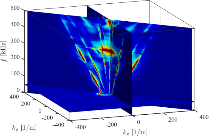
Wavenumber-wavenumber-frequency data sliced at 45° and 90° of wave propagation angles.
-
Slicing 3D data at chosen frequencies - creating a set of angular profiles (Fig. 4).
Fig. 4. 
Wavenumber-wavenumber-frequency data sliced at two chosen frequencies.


For dispersion curves optimization process seven various propagation angles \( \beta \) were used, namely: 0°, 15°, 30°, 45° 60°, 75°, and 90°. Final dispersion curves drawn on experimental data with white lines for chosen propagation angles are presented in Fig. 5.

Dispersion curves for chosen propagation angles.
Very good agreement between experimental and numerical dispersion curves have been observed for all tested propagation angles.
In the second proposed approach in which numerical angular profiles where optimized to match experimental data, seven various frequencies were used, namely: 48.85, 98.94, 149.04, 199.14, 249.24, 299.33, and 349.43 kHz. Final numerical angular profiles after the optimization process are drawn with white lines on experimental data and presented for chosen frequencies in Fig. 6. Very good agreement between numerical and experimental data has been achieved for all modes at all tested frequencies.

Angular profiles for chosen frequencies.
Due to symmetry in the wave propagation, only the area corresponding to positive wavenumbers was used in both optimization processes.
Elastic constants estimated for the same CFRP sample with two presented techniques are given in Table 1. Similar results were obtained for most elastic constants beside C33 and C66. The difference of around 10% is non-negligible, and without additional tests with other techniques, it is impossible to determine which results are closer to the real specimens elastic constants. Further verification tests are planned in future.
6 Conclusions
In this work, a technique for elastic constants identification based on Lamb wave propagation measurement is presented. Two approaches for the optimization are proposed. SASE model and full wavefield measurements along with the genetic algorithm are used in the optimization process. In both cases, a very good agreement between numerical and experimental data has been reached. However, the optimization of dispersion curves was computationally more efficient than the optimization of angular profiles. The time needed for a single genetic algorithm run was about ten times shorter for the former. It should be noted that estimated elastic constants for the same specimen using both approaches have some discrepancies and additional testing with another technique should be used to determine which results were closer to the real values. Such studies are planned in the future.
References
Wang, W., Kam, W.: Material characterization of laminated composite plates via static testing. Compos. Struct. 50, 347–352 (2000)
Wesolowski, M., Barkanov, E., Rucevskis, S., Chate, A., La Delfa, G.: Characterisation of elastic properties of laminated composites by nondestructive techniques. In: ICCM International Conferences on Composite Materials, Edinburgh (2009)
Rose, J.L., Ditri, J.J., Huang, Y., Dandekar, D.P., Chou, S.C.: One-sided ultrasonic inspection technique for the elastic constant determination of advanced anisotropic materials. J. Nondestruct. Eval. 10, 159–166 (1991)
Martens, A., Kersemans, M., Daemen, J., Verboven, E., Van Paepegem, V., Delrue, S., Van Den Abeele, K.: Characterization of the orthotropic viscoelastic tensor of composites using the Ultrasonic Polar Scan. Compos. Struct. 230, 111499 (2019)
Ong, W., Rajic, N., Chiu, W., Rosalie, C.: Determination of the elastic properties of woven composite panels for Lamb wave studies. Compos. Struct. 141, 24–31 (2016)
Kudela, P., Radzienski, M., Fiborek, P., Wandowski, T.: Elastic constants identification of woven fabric reinforced composites by using guided wave dispersion curves and genetic algorithm. Compos. Struct. 249, 112569 (2020)
Bartoli, I., Marzani, A., Lanza di Scalea, F., Viola, E.: Modeling wave propagation in damped waveguides of arbitrary cross-section. J. Sound Vibrat. 295, 685–707 (2006)
Taupin, L., Lhemery, A., Inquiete, G.: A detailed study of guided wave propagation in a viscoelastic multilayered anisotropic plate. J. Phys: Conf. Ser. 269, 012002 (2011)
Chipperfield, A., Fleming, P., Pohlheim, H., Fonseca, M.: Genetic Algorithm Toolbox User’s Guide, Technical report, University of Shefield (1994)
Acknowledgments
The research was funded by the Polish National Science Center under grant agreement no 2018/29/B/ST8/00045.
Author information
Authors and Affiliations
Corresponding author
Editor information
Editors and Affiliations
Rights and permissions
Copyright information
© 2021 Springer Nature Switzerland AG
About this paper

Cite this paper
Radzieński, M., Kudela, P., Wandowski, T., Ostachowicz, W. (2021). Strategies for Identification of Elastic Constants in Highly Anisotropic Materials Using Lamb Waves. In: Rizzo, P., Milazzo, A. (eds) European Workshop on Structural Health Monitoring. EWSHM 2020. Lecture Notes in Civil Engineering, vol 127. Springer, Cham. https://doi.org/10.1007/978-3-030-64594-6_75
Download citation
DOI: https://doi.org/10.1007/978-3-030-64594-6_75
Published:
Publisher Name: Springer, Cham
Print ISBN: 978-3-030-64593-9
Online ISBN: 978-3-030-64594-6
eBook Packages: EngineeringEngineering (R0)