
Abstract
Parallelization is the process of finding instruction clusters called tasks, which can be executed in concurrent fashion, on multiple processing elements. The objective of parallel execution is to reduce program run time, by overlapping the processing of these tasks. However these tasks are not entirely independent, and generally depend on data generated by peers. One of the objectives of effective parallelization is to limit this inter-task communication, an overhead which can limit the speedup realized through parallelization. Since this inter-task communication cannot be entirely avoided, judiciously mapping the tasks among the processors of a parallel machine, assumes utmost importance. Performance of a parallel program, is also determined by how uniformly the processors of the target machine are loaded with tasks, in situations where the tasks outnumber the processors. This activity is normally referred to as the load balancing. The problem of generating parallel tasks out of a sequential program is well studied, but the related problem of effectively mapping the concurrent tasks, to the processors of a parallel machine, still needs to be researched. This research work involved studying the problem of mapping specific tasks to individual processors, referred to here as the Processor Task Mapping and finding effective solutions. Previous solutions to the mapping problem were non-deterministic, sub-optimal, and incomplete, since their focus was mainly on the task schedules and load balancing criteria and mostly ignoring the communication profile of the tasks to drive the mapping decision. This was the main driving force for taking up our research. We present here the outcomes of this study namely, several efficient graph based algorithms to perform this mapping effectively. These algorithms are general and are applicable to machine topologies of diverse architectures, including the Shared Memory Multiprocessor, Distributed Multiprocessor and the Non-Uniform Memory Access Machines (NUMA), are scalable, deterministic, and produce close to optimal solutions.
Access provided by Autonomous University of Puebla. Download conference paper PDF
Keywords
- Parallelization
- Topology
- Task
- Mapping
- NUMA
- Distributed
- Communication
- Algorithm
- Graph based algorithms
- HPC
- High Performance Computing
- Compiler Optimization
1 Introduction
Parallel machines are characterized, by the number of processing elements, and the different ways these processors can be interconnected. Since the prime reason for using a parallel machine is to share the software workload, the configuration which includes both the processors and the interconnection network mainly determines the performance one can expect from the parallel machine. This ultimately dictates how the machine scales, in relation to larger problem sizes and the resulting addition to the processor count.
The interconnection networks are diverse in nature, dictated by performance considerations, physical design, and implementation, and are collectively referred to as the Processor Interconnect Topology. Historically the published literature presents several references to processor interconnect topologies [5, 7]. Some of the popular ones include the Shared Bus, Fully Connected Network, Linear Array, Ring, Mesh, Tori, Grid, Cube, Tree, Fat Tree, Benes Network, and Hypercube among others. The following sections look at some of them in detail, and also provide a mathematical abstraction for representing them, and using them in analysis.
The computation in a higher level language program can be represented internally in a compiler, by a representation such as a three address form [15]. The dependencies that exist between statements or instructions of the program, manifest in two forms namely, Data Dependence and Control Dependence [17, 29]. Data dependence exists between two instructions, when one of them reads a datum that the other has written. Control dependence exists between two instructions, when the execution of one of them is conditional on the results produced by the execution of the other. There are several mathematical representations available to represent a program internally, but the Program Dependence Graph (PDG) is a popular technique that captures these program artifacts [8]. PDG is a convenient tool to partition a sequential program into parallel tasks [11, 12, 15, 16, 28]. While detection of parallelism in software is a popular area of research, it is not central to the topic we have chosen for our research work here. We start with the assumption that the concurrent tasks are available and focus on the related problem of mapping them to available processors. The main research goal is to find out if the choice of a processor for a particular task makes a difference to the overall efficiency of the mapping process.
The problem of assigning parallel tasks of a program, to processors of a distributed system efficiently, is referred to here as the Task Assignment Problem. An effective solution to this problem normally depends on the following criteria namely, Load Balancing and Minimization of Communication Overhead. Load Balancing is a process, where the computing resources of a distributed system are uniformly loaded, by considering the execution times of the parallel tasks. Existing load balancing strategies can be broadly classified as static and dynamic, based on when the load balancing decision is made. In static methods, the load balancing decision is taken at the task distribution time and the assignment of tasks to processors remains fixed for the duration of their execution [27]. On the other hand, the dynamic schemes are adaptive to changing load conditions and tasks are migrated as necessary, to keep the system balanced. The latter scheme is more sensitive to changing topological characteristics of the machine, especially the communication overheads [20].
Minimization of communication overhead involves clustering the tasks carefully on the target machine, so as to minimize the inter-task communication demands. There are two factors influencing this decision namely, the communication granularity and the topological characteristics of the underlying distributed machine [14]. Task assignment is not an easy problem to solve, since load balancing and communication minimization are inter-related, and improving one adversely affects the other. This is believed by many to be an NP Complete problem [2]. There are solutions proposed in the literature based on Heuristics and other search techniques [3]. However missing are efficient algorithms that are scalable, complete, and deterministic.
Typically, mapping problems that involve binary relations could be represented and studied by creating a model based on graphs. Topology representation is a problem that can be modeled as a graph, with processors as nodes and edges representing the processor connections. The tasks could also be represented as a graph, with tasks as nodes and edges denoting the communication between them. The solution would then be the mapping of the task nodes to the suitable nodes of the processors. This would require solutions to several sub-problems such as the following: How to gather the various properties of a graph, such as the node and edge count, individual connections, clustering, weights, etc.? How do we capture graph similarities? The obvious way of course is by visual inspection, which works for manageable sizes, but not for real world large graphs. Is it possible to solve this problem, in a deterministic fashion? [26] is a good survey paper, on the topic of graph comprehension and cognition.
This research work involves studying, and developing a methodology, to map parallel tasks of any given program, to a suitable processor topology in linear or near linear time. Subsequent sections provide more details of the findings, including several algorithms, that produce task assignments, that are designed to be progressively more efficient than the earlier algorithms.
In Sect. 1, we look at existing solutions to the task mapping problem, highlight the deficiencies in the current solutions, and elaborate on the motivations for pursuing our research work. In Sect. 2, we discuss the various popular ways of connecting the processors of a distributed machine and a suitable mathematical representation for each. Section 3 defines the Task Assignment Problem, which is the topic of investigation in this work. In Section 4 we present the various mapping algorithms proposed in this paper. In Sect. 5, we theoretically examine the fitness of each algorithm, in terms of its run time complexity. In Sect. 6, the final section of the paper, we conclude the paper by revisiting the motivations for taking up our research work, and briefly summarizing our findings and contributions with some ideas for extending the work for the future.
2 Related Works
Historically, researchers have used graphs to represent processor and network topologies [31]. Such a graph has been used to compute robustness of a network, towards corruptions related to noise and structural failures [1].
How do we capture both the topology and task details in a single graph? We found several references on the topic of graph aggregation, and incremental graph construction, subject to certain constraints. One such idea is a topological graph constrained by a virtual diameter, signifying properties such as communication [10]. However they do not provide implementation details. Researchers have used the spectral filtering techniques for analyzing network topologies, using Eigen vectors to group similar nodes in the topology, based on geography or other semantic properties [9]. Comparing directed graphs, including those of different sizes by aggregating nodes and edges, through deterministic annealing has been studied [30]. Graph aggregation techniques based on multi-dimensional analysis for understanding of large graphs have been proposed [25].
Graph Summarization is a process of gleaning information out of graphs for understanding and analysis purposes. Most of the methods are statistical in nature which use degree distributions, hop-plots, and clustering coefficients. But statistical methods are plagued by the frequent false positive problem and so are other methods. Analytical methodologies on the other hand are immune to such limitations [25].
Load Balancing on Distributed Systems has been studied extensively for a long time, and a plethora of papers exist on this topic [4, 6, 20, 23, 24, 27]. However load balancing is just one of the criteria that determines efficient performance of a distributed application. It needs to be complemented with minimization of communication overheads to see positive performance results.
Several researchers have tackled the task assignment problem before with varying degree of success. One such solution to the problem, based on the genetic algorithm technique in the context of a Digital Signal Processing (DSP) system has been proposed [3]. Researchers have used duplication of important tasks among the distributed processors to minimize communication overheads and generate efficient schedules [2]. Methods using the Message Passing Interface (MPI), on to a High Performance Computing (HPC) machine with Non-Uniform Memory Access (NUMA) characteristics, using a user supplied placement strategy has been tried by several groups with effective results [13, 14]. A few researchers have used both load balancing and communication traits as criteria to drive the mapping decisions [22]. They use dynamic profiling, to glean performance behavior of the application. However dynamic profiling is heavily biased on the sample data used and in our opinion, static analysis of the communication characteristics is a better technique and should yield optimum results in most situations.
Besides the domain of Parallel Processing, are there other fields where the task mapping problem has been explored? Assignment of Internet services based on the topology and the traffic demand information is one such domain [21]. Mapping tasks to processing nodes has also been studied at length, by researchers working in the Data Management domain. Tasks in a Data Management System, are typically characterized by data shuffling and join operations. This demands extra care in parallelization besides static partitioning, such as migrating tasks to where data is to realize maximum benefit [19]. Query processing is another area, where static partitioning of tasks runs into bottlenecks, and the authors solve this by running queries on small fragments of input data, whereby the parallelism is elastically changed during execution [18]. However our solution to the mapping problem is a general technique, and is not specific to the Data Management problem or the Internet domain and should be easily adaptable here.
In this research work, we propose a mathematical representation, based on directed graphs, to represent both the machine topology and the parallel task profiles. These graphs are then read by our task mapper, to map the processors and tasks. The following sections look at the problem and solutions in greater detail.
3 Processor Interconnection Topologies
Processors in a Multiprocessor machine can be interconnected in several interesting ways that mainly affect how the resulting machine scales as processors are added. It is important both from a problem representation and solution perspective, that we study these topologies in some detail and understand them. We next discuss several popular processor interconnection topologies found in published literature, and show with the help of diagrams, how each of these topologies could be represented mathematically as directed graphs.
At one end of the spectrum is the Shared Bus, where at any given time, a single communication is in progress. At the other end lies the Fully Connected Network, where potentially at any given time, all the processors could be involved in private communication. If the number of processors in the network is N, with a shared bus we can only realize a bandwidth of O(1), but with a fully connected network, we could extract a bandwidth of O(N) [5, 7]. There are several other topologies that fall in between, and we will look at a few of them in the following paragraphs.
Figure 1a, b on page 471 illustrates a simple bus topology, for connecting processors of a machine and its graph representation. Likewise a Linear Array is a simple interconnection of processor nodes, connected by bidirectional links. Figure 2a, b on page 471 represents linear topology and its corresponding graph.

Shared bus (a) topology and its (b) graph

Linear bus (a) topology and its (b) graph
A Ring or a Torus is formed from a Linear Array, by connecting the ends. There is exactly one route from any given node to another node. Figure 3a on page 472 is an illustration of a topology organized in the form of a ring, which allows communication in one direction between any pair of nodes. The associated Fig. 3b on page 472 illustrates how the topology can be represented as a graph. The average distance between any pair of nodes in the case of a ring is N∕3 and in the case of a Linear Array it is N∕2, where N is the number of nodes in the network. We could potentially realize a bandwidth of O(N), from such a connection.

Ring bus (a) topology and its (b) graph
Grid, Tori, and Cube are higher dimensional network configurations, formed out of Linear arrays and Rings. Specifically they are K-ary, D-cube networks with K nodes, in each of the D dimensions. These configurations provide a practical scalable solution packing more processors in higher dimensions. To travel from any given node to another, one crosses links across dimensions, and then to the desired node in that dimension. The average distance traveled in such a network is D ∗ (2∕3) ∗ K.
The most efficient of all the topologies in terms of the communication delays is the fully connected network with edges, connecting all possible pairs of nodes. In this connection topology, there is just the overhead introduced due to propagation, but no additional overheads introduced by nodes that lie in the path between any pair of nodes. However the implementation of such a topology is quite complex. Figure 4a, b on page 473 represents the fully connected topology and its corresponding graph.

Fully connected (a) topology and its (b) graph
Figure 5a, b on page 473 illustrates the Star topology and its graph, where there is a routing node in the middle, to which the rest of the nodes in the machine are connected. This configuration provides a solution that is somewhat less efficient in time, but is less complex to implement.

Star (a) topology and its (b) graph
Binary trees represent another efficient topology with logarithmic depth, which can be efficiently implemented in practice. A network of N nodes offers an average distance of N ∗ Log(N).
Based on the sample topologies presented earlier, it should be obvious to the reader that any complex topology can be modeled as a graph. It should also be noted that all graphs representing topologies, including those that are not fully connected, should allow a path between any pairs of nodes, even though not directly connected, by a route that passes through other intermediary nodes.
4 Task Assignment Problem
The problem of assigning parallel tasks of a program to the processing elements of a suitable machine topology is referred to here as the Task Assignment Problem. The characteristics of the machine relevant for the assignment, is captured in a graph, which we refer to here, as the Processor Topology Graph (PTG). The nodes of such a graph represent the processors and the edges represent the connections between the processors. The nodes could include parameters that capture processor characteristics, such as the clock rate. Similarly, the edge parameters could capture the bandwidth details of the connection, both of which could serve to drive the placement decisions. The communication details pertaining to the tasks can be captured in another graph, which we refer to as the Task Communication Graph (TCG). The nodes of the TCG represent the tasks and node parameters could represent the computation cycles for the task. The edges denote the communication that exists between any pair of tasks and the edge parameters could represent the volume of communication if any between the tasks concerned. Both the node and edge parameters could provide input for the placement algorithms. A Task Assignment Graph (TAG) captures the augmented information, from both the PTG and TCG, that mainly conveys the task to processor mappings.
In summary, the task assignment problem could be defined as a selective process whereby a particular processor is chosen among a list of available processors to act as a host for executing a particular task. For clarification purposes, a task is just a collection of executable instructions grouped together for the purpose of convenience. We propose the following algorithms, to solve the Task Assignment Problem:
-
1.
Minima_Strategy: Uses a random mapping strategy
-
2.
Maxima_Strategy: Provides a topology with direct connections between processors
-
3.
Dimenx_Strategy: Focuses on either the cycle or bandwidth requirement of tasks
-
4.
Dimenxy_Strategy: Considers both the task cycles and bandwidth requirement
-
5.
Graphcut_Strategy: Creates subgraphs out of the topology and task graphs and maps them
-
6.
Optima_Strategy: Maps tasks to a virtual topology and then remaps to an actual physical topology
-
7.
Edgefit_Strategy: Sorts the edges of the topology and task graphs and maps the best edges
The following subsections provide the details of each one of these algorithms.
5 Task Mapping Algorithms
This section provides algorithmic details of each of the algorithms which follows a summary or objective of the algorithm.
-
1.
Minima_Strategy Algorithm: This is a very simple scheme where in the list of processors in PTG, as well as the list of tasks in the TCG are randomly shuffled as a first step. Then the tasks in the shuffled TCG are assigned to processors, in the shuffled PTG in a random fashion one-on-one. While this scheme does not guarantee efficient task placements, we can definitely use the result in comparisons, for measuring the effectiveness of other strategies.
Algorithm 1 on page 475 provides the steps required to implement the Minima Strategy algorithm.
Algorithm 1 Minima_Strategy algorithm

-
2.
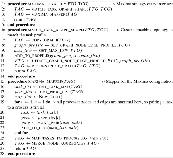
Task Mapping by Maxima_Strategy: The objective of this algorithm is to provide a topology that produces maximum benefits to the set of tasks from a topology standpoint. It achieves this by providing direct connections to the tasks so that the communicating tasks need not experience router and other network delays.
Algorithm 2 on page 476 provides the steps required to implement the Maxima_Strategy algorithm.
Algorithm 2 Maxima_Strategy algorithm
-
3.
Dimenx_Strategy algorithm: There are actually two sub-strategies here. One that takes into consideration the task execution cycles and another that considers the task communication bandwidth. Accordingly, the algorithm uses a depth-first-listing of processors to achieve the first objective where the underlying assumption is that processor connection is not important so we can afford to map to processors that are farther apart in the topology. To achieve criteria two, the algorithm maps tasks to a breadth-first-listing of processors since the direct connection between processors would be required.
Algorithm 3 on page 477 provides the details necessary to implement Dimenx_Strategy of mapping tasks to processors.
Algorithm 3 Dimenx_Strategy algorithm

Algorithm 4 Dimenx_Strategy algorithm (cont…)

-
4.
Dimenxy_Strategy algorithm:
The Dimenxy strategy algorithm tries to achieve two demands of the tasks at the same time, by maximizing the computation part, and controlling the communication overheads, by minimizing the communication to computation ratio, through effective mapping of tasks to processors. Tasks are grouped into clusters referred to here as segments, based on their inherent nature, whether computation or communication biased, and then mapped accordingly segmentwise.
Algorithm 5 on page 479 describes the Dimenxy_Strategy Algorithm for generating the TAG.
Algorithm 5 Dimenxy_Strategy algorithm

Algorithm 6 Dimenxy_Strategy algorithm (cont…)

-
5.
Graphcut_Strategy algorithm:
Graphcut Strategy algorithm, creates subgraphs out of PTG and TCG that are matching or similar from a shape perspective, and so can be easily mapped. It is important to slice a graph only to the extent that we get subgraphs that are similar in shape, and more amenable for mapping. The subgraphs are similar in shape, in terms of the number of nodes constituting the subgraphs, and the number of edges, and the number of edges incident and leaving the nodes of the concerned subgraphs. One should be careful not to take this slicing too far, in which case we can end up with a graph of just nodes, with no shape or edge information, making the mapping decisions difficult.
Algorithm 7 on page 481 describes the Graphcut_Strategy Algorithm for generating the TAG.
Algorithm 7 Graphcut_Strategy algorithm
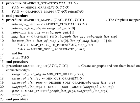
Algorithm 8 Graphcut_Strategy algorithm (cont…)

-
6.
Optima_Strategy algorithm:
The Optima_Strategy algorithm follows a two step process where the sorted edges of the TCG are mapped to a virtual topology with no processor limitations. Then the second mapping step is carried out using node sorted graphs of topology and task graphs.
Algorithm 9 Optima_Strategy algorithm
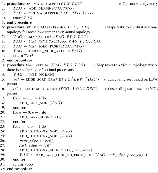
Algorithm 10 Optima_Strategy algorithm (cont…)

-
7.
Edgefit_Strategy algorithm:
Edgefit_Strategy involves mapping the task edge with the highest communication volume, with the topology edge with the highest bandwidth, and so on. This seems like an easy task to achieve, but practically poses consistency issues, because a task can only be mapped, to a single processor at any time. So an extra post processing step is required, whereby inconsistent mappings have to be sorted out.
Algorithm 11 on page 484 describes the Edgefit_Strategy Algorithm for generating the TAG.
Algorithm 11 Edgefit_Strategy algorithm

Algorithm 12 Edgefit_Strategy algorithm (cont…)


We presented seven algorithms with varying degree of complexity in terms of implementation and accordingly offer varying levels of performance. So which algorithm offers maximum benefit for a particular scenario? Minima strategy is simple to implement and may work well in many situations, especially when there are few processors in the topology and a large number of tasks. Since Maxima strategy uses direct connections between processors, it provides an upper limit on the maximum performance level possible, for any combination of processors and tasks. Dimenx and Dimenxy are good strategies to employ in situations, when both the tasks cycles and bandwidth dictate performance. Graphcut, Optima, and Edgefit are complex strategies to implement and run, and should be employed for complex processor topologies and large task counts, where communication volumes and bandwidth expectations are high. In such scenarios the extra time spent, in carefully mapping tasks to the appropriate processors, translates to measurable performance benefits and is definitely worth the effort.
6 Complexity Analysis of the Algorithms
In this section, we look at the complexity of the algorithms proposed in this paper. We use the standard Big − O notation, which defines the upper bounds, on the scalability of algorithms in general. The O on the left hand side in each of these equations stands for the Big − O measure. The purpose of providing these equations is mainly to acquaint the readers about the complexity of the algorithms presented earlier and provide mathematically an expectation in terms of performance. In this study we have focused on the time complexity of the algorithms using the Big − O notation. Since we believe that the algorithms are moderate in their use of memory, we chose not to discuss or analyze their space complexity behavior at this point.
-
1.
Minima_Strategy: The algorithm is simple. It just maps every task in the set randomly with a processor in the topology. So there is just one loop which picks a task in sequence from the list of tasks and maps with a processor it has randomly chosen from the list of processors. If you ignore the work done in generating the lists from their corresponding graphs PTG and TCG, the complexity is just O(N) where N is the number of tasks.
$$\displaystyle \begin{aligned} O(Minima) = O(N) \end{aligned} $$(1)where N is the number of tasks.
-
2.
Maxima_Strategy: Initialization involves finding the maximum value of bandwidth which means looping through the list of processor edges which translates to a complexity of O(E) where E is the number of edges in the original topology. It also involves creating a processor topology that produces the best results for the given task set. This involves creating processor nodes and edges mimicking the task graph. This means an additional complexity of O(N) where N is the number of nodes in the task set. Another order of O(N 2) where we are setting up direct edges between any pair of tasks for realizing the best communication results.
$$\displaystyle \begin{aligned} O(Maxima) = O(N) + O(N^{2}) + O(E) \end{aligned} $$(2)where N is the number of tasks, E is the number of topology edges.
-
3.
Dimenx_Strategy: Finding the Dfs listing of all the processors in the topology which involves looping through the nodes and for each node follow each direct edge and visit them in turn which translates to an order of O(EN) where E is the number of processor edges and N is the number of processor nodes. Finding a descending order listing of all task nodes based on the execution cycles translates to O(M 2) when using a simple bubble sort where M is the number of task nodes. Mapping processors to tasks is O(M) like before where M is the number of tasks. So totally we have,
$$\displaystyle \begin{aligned} O(Dimenx_{C}) = O(EN) + O(M^{2}) + O(M) \end{aligned} $$(3)where M is the number of tasks and N is the number of processors and E is the number of processor edges.
Similarly when we use Volume as the reference we have a task edge sorting step which is the only step that is different from above. So in total we have,
$$\displaystyle \begin{aligned} O(Dimenx_{V}) = O(EN) + O(F^{2}) + O(M) \end{aligned} $$(4)where M is the number of tasks and N is the number of processors, E is the number of processor edges, and F is the number of task edges.
-
4.
Dimenxy_Strategy: Involves the generation of both the Dfs and Bfs listing of the processors in the topology. As explained earlier, this translates to a complexity of O(EN) each. Computing aggregate volumes is aggregating edge weights in the task nodes which is of complexity O(F), where F is the number of edges in the task graph. Sorting the task nodes based on their communication volumes is a O(M) where M is the number of task nodes. Mapping is a O(M) order where M is the number of task nodes.
$$\displaystyle \begin{aligned} O(Dimenxy) = O(EN) + O(F) + 2 * O(M) \end{aligned} $$(5)where M is the number of tasks, N is the number of processors, E is the number of processor edges, and F is the number of edges in the task graph.
-
5.
Graphcut_Strategy: Graph cut step which is a O(EM) where E is the number of edges and M is the number of nodes in the processor topology graph. Similarly for the task graph this step is a O(FN) order of complexity. The sort of the list of subgraphs of PTG is a worst case order of O(M 2) where M is the number of nodes in the processor topology. Similarly for tasks it is a O(N 2) where N is the number of task nodes. Matching the subgraphs and the nodes within corresponding subgraphs is a O(N 2) order where N is the number of task nodes. So in total we have,
$$\displaystyle \begin{aligned} O(Graphcut) = O(EM) + O(FN) + O(M^{2}) + 2 * O(N^{2}) \end{aligned} $$(6)where N is the number of tasks and M is the number of processors, E is the number of processor edges and F is the number of task edges.
-
6.
Optima_Strategy: Map virtual step involves building a virtual graph that has the same number of processor nodes and number of edges equal to the number of edges in the task graph. The mapping step involves going through the list of task edges and mapping the virtual processors one on one. This translates to the following, O(M) + 2 ∗ O(F) where M is the number of processor nodes and F is the number of task edges. Mapping to a physical topology involves aggregating edge properties to nodes in the topology and task graphs which translates to O(E) + O(F) where E is the number of edges in PTG and F in TCG. Two node sort operations of the PTG and TCG graphs are of order O(M 2) and O(N 2) respectively, where M is the number of nodes in PTG and N the corresponding number in TCG. Mapping edge is a O(NF) in the worst case where N is the number of task edges and F is the edges that involve a particular task node. Totally this translates to
$$\displaystyle \begin{aligned} O(Optima) = O(M) + 3 * O(F) + O(E) + O(M^{2}) + O(N^{2}) + O(NF) \end{aligned} $$(7)where N is the number of task nodes and M is the number of processor nodes, E is the number of PTG edges and F the number of TCG edges.
-
7.
Edgefit-Strategy: The edge sort steps of PTG and TCG are of order O(E 2) and O(F 2) as discussed earlier, where E is the number of processor edges and F the number of task edges. Mapping of edges in greedy fashion is of order O(F), where F is the number of edges in TCG. Backtrack which involves comparison of one edge with another is a O(F 2) order where F is the number of edges in the task graph. The Task-per-processor (for load balancing) values gathering step is a O(M), where M is the number of processors. Together they are 3 ∗ O(M). Migrate step involves finding a suitable processor for the migrating task and its worst case order is O(M), where M is the number of processors. Balance step involves sorting the processor graph once and looping till all processors are balanced, and each time in the loop balance the load-balance checks are called. This translates to O(M 2) + O(M ∗ (4 ∗ M)) and we have the following equation:
$$\displaystyle \begin{aligned} O(Edgefit) = O(E^{2}) + O(F) + O(F^{2}) + 5 * O(M^{2}) \end{aligned} $$(8)
7 Preliminary Results
This section gives some preliminary results on the performance of the various algorithms, for a configuration that consists of a topology of 512 processors and 1024 tasks. This configuration was generated by a tool, where in the processors connections were randomly chosen, as well as the bandwidth of the connections. The topology is not a fully connected one, but all processors are connected, with some of them with direct connections and others with indirect connections, enabled by one or more intermediate processors. Similarly, the communicating tasks and non-communicating tasks were randomly chosen, as also the volume of the communication in the former case. The bandwidths across processor boundaries were determined through simulation. The result has been captured in the form of a table and a plot below. While the actual simulation values are not relevant for this discussion, both the line bandwidth and task communication volumes were randomly generated for this experiment and they were generated in the form of a comma-separated-value files and stored as parameters in the appropriate graphs such as the PTG or the TCG as relevant. The algorithms used these bandwidths to guide the task placements and at the end they were evaluated based on the overall bandwidth overheads they were able to achieve in the topology. Less overheads mean better placement and translates to a better network/bandwidth efficiency.
Detailed analysis, results, and plots are planned to be presented in a separate work which is an extension to the present research.
Table 1 on page 488 lists the bandwidth overheads experienced by the algorithms for an example configuration that involves a topology of 512 processors and 1024 tasks. As seen from the table, we see that MAXIMA configuration has achieved the best/lowest overhead as expected along with OPTIMA. We also see that the highest overhead for this particular experiment was grabbed by GRAPHCUT which needs further study to determine the causes. The middle values are grabbed by the others.
Figure 6 on page 488 lists the bandwidth overheads experienced by the algorithms for an example configuration that involves a topology of 512 processors and 1024 tasks. The plot basically conveys the same information as the table in a graphical format. And we can see that MAXIMA algorithm has done better than the others in limiting the bandwidth overheads by mapping tasks and processors effectively.

Bandwidth overheads experienced by the algorithms
8 Conclusion
In this research work, we studied the problem of mapping parallel tasks of a program to the processors of a multiprocessor machine. The problem is interesting and challenging, since effective mapping depends on two criteria, namely the total execution cycles consumed by each processor and the overall bandwidth provided to the tasks by the topology. Effective use of processing resources of machine is possible by distributing the tasks across multiple processors which also serves the load balancing cause. To effectively use the bandwidth resources of a topology, more work is required to effectively choose processors for the tasks. We characterized this problem as the task assignment problem. We presented the following seven algorithms to solve the problem, based on the mathematical abstraction of a graph: Minima_Strategy, Maxima_Strategy, Dimenx_Strategy, Dimenxy_Strategy, Graphcut_Strategy, Optima_Strategy, and Edgefit_Strategy. These algorithms read the topology and task profiles, in the form of two weighted directed graphs namely, the Processor Topology Graph (PTG) and the Task Communication Graph (TCG), and generate a Task Assignment Graph (TAG), also a directed graph as output with the required task to processor mappings. These algorithms are general and are applicable to a wide range of machine architectures, including distributed multiprocessors such as NUMA. Future work involves characterizing these algorithms based on their performance and development of a tool or infrastructure to study and manage topologies and task profiles, as well as design custom topologies for optimum performance.
References
Abbas W, Egerstedt M (2012) Robust graph topologies for networked systems. IFAC Proc Vol 45(26):85–90 (2012). https://doi.org/https://doi.org/10.3182/20120914-2-US-4030.00052, http://www.sciencedirect.com/science/article/pii/S147466701534814X. 3rd IFAC workshop on distributed estimation and control in networked systems
Ahmad I, Kwok YK (1998) On exploiting task duplication in parallel program scheduling. IEEE Trans Parallel Distrib Syst 9(9):872–892. https://doi.org/10.1109/71.722221
Ahmad I, Dhodhi MK, Ghafoor A (1995) Task assignment in distributed computing systems. In: Proceedings international phoenix conference on computers and communications, March 1995, pp. 49–53. https://doi.org/10.1109/PCCC.1995.472512
Chou TCK, Abraham JA (1982) Load balancing in distributed systems. IEEE Trans Softw Eng 8(4):401–412
Culler D, Singh JP, Gupta A (1998) Parallel computer architecture: a hardware/software approach. Morgan Kaufmann Publishers Inc., San Francisco
e Silva EDS, Gerla M (1991) Queueing network models for load balancing in distributed systems. J Parallel Distrib Comput 12(1):24–38
Feng TY (1981) A survey of interconnection networks. Computer 14(12):12–27
Ferrante J, Ottenstein KJ, Warren JD (1984) The program dependence graph and its use in optimization. In: Proceedings of the 6th colloquium on international symposium on programming. Springer, London, pp 125–132. http://dl.acm.org/citation.cfm?id=647326.721811
Gkantsidis C, Mihail M, Zegura E (2003) Spectral analysis of internet topologies. In: INFOCOM 2003. Twenty-second annual joint conference of the IEEE computer and communications. IEEE societies, vol 1. IEEE, New York, pp 364–374
Grieco LA, Alaya MB, Monteil T, Drira K (2014) A dynamic random graph model for diameter-constrained topologies in networked systems. IEEE Trans Circ Syst II: Express Briefs 61(12):982–986. https://doi.org/10.1109/TCSII.2014.2362676
Horwitz S, Reps T (1992) The use of program dependence graphs in software engineering. In: International conference on software engineering, 1992, pp 392–411. https://doi.org/10.1109/ICSE.1992.753516
Horwitz S, Reps T, Binkley D (1990) Interprocedural slicing using dependence graphs. ACM Trans Program Lang Syst 12(1):26–60. http://doi.acm.org/10.1145/77606.77608
Hursey J, Squyres JM, Dontje T (2011) Locality-aware parallel process mapping for multi-core HPC systems. In: 2011 IEEE international conference on cluster computing, September, pp 527–531. https://doi.org/10.1109/CLUSTER.2011.59
Jeannot E, Mercier G (2010) Near-optimal placement of MPI processes on hierarchical NUMA architectures. In: D’Ambra P, Guarracino M, Talia D (eds) Euro-Par 2010 - parallel processing. Springer, Berlin, Heidelberg, pp 199–210
Kalyur S, Nagaraja GS (2016) ParaCite: auto-parallelization of a sequential program using the program dependence graph. In: 2016 international conference on computation system and information technology for sustainable solutions (CSITSS), October, pp. 7–12. https://doi.org/10.1109/CSITSS.2016.7779431
Kalyur S, Nagaraja GS (2017) Concerto: a program parallelization, orchestration and distribution infrastructure. In: 2017 2nd international conference on computational systems and information technology for sustainable solution (CSITSS), December, pp 1–6. https://doi.org/10.1109/CSITSS.2017.8447691
Kennedy K, Allen JR (2002) Optimizing compilers for modern architectures: a dependence-based approach. Morgan Kaufmann Publishers Inc., San Francisco
Leis V, Boncz P, Kemper A, Neumann T (2014) Morsel-driven parallelism: a NUMA-aware query evaluation framework for the many-core age. In: Proceedings of the 2014 ACM SIGMOD international conference on Management of data. ACM, New York, pp 743–754
Li Y, Pandis I, Mueller R, Raman V, Lohman GM (2013) NUMA-aware algorithms: the case of data shuffling. In: CIDR
Loh PKK, Hsu WJ, Wentong C, Sriskanthan N (1996) How network topology affects dynamic load balancing. IEEE Parallel Distrib Technol 4(3):25–35. http://dx.doi.org/10.1109/88.532137
Pantazopoulos P, Karaliopoulos M, Stavrakakis I (2014) Distributed placement of autonomic internet services. IEEE Trans Parallel Distrib Syst 25(7):1702–1712
Pilla LL, Ribeiro CP, Cordeiro D, Bhatele A, Navaux PO, Méhaut JF, Kalé LV (2011) Improving parallel system performance with a NUMA-aware load balancer. Tech. rep.
Shirazi BA, Kavi KM, Hurson AR (1995) Scheduling and load balancing in parallel and distributed systems. IEEE Computer Society Press, Los Alamitos (1995)
Tantawi AN, Towsley D (1985) Optimal static load balancing in distributed computer systems. J ACM 32(2):445–465
Tian Y, Hankins RA, Patel JM (2008) Efficient aggregation for graph summarization. In: Proceedings of the 2008 ACM SIGMOD international conference on management of data. ACM, New York, pp. 567–580
Von Landesberger T, Kuijper A, Schreck T, Kohlhammer J, van Wijk JJ, Fekete JD, Fellner DW (2011) Visual analysis of large graphs: state-of-the-art and future research challenges. In: Computer graphics forum, vol 30. Wiley Online Library, pp 1719–1749
Wang YT et al (1985) Load sharing in distributed systems. IEEE Trans Comput 100(3):204–217
Weiser M (1984) Program slicing. IEEE Trans Softw Eng SE-10(4):352–357. https://doi.org/10.1109/TSE.1984.5010248
Wolfe M, Banerjee U (1987) Data dependence and its application to parallel processing. Int J Parallel Programm 16(2):137–178
Xu Y, Salapaka SM, Beck CL (2014) Aggregation of graph models and Markov chains by deterministic annealing. IEEE Trans Autom Control 59(10):2807–2812
Zegura EW, Calvert KL, Donahoo MJ (1997) A quantitative comparison of graph-based models for internet topology. IEEE/ACM Trans Network 5(6):770–783
Author information
Authors and Affiliations
Corresponding author
Editor information
Editors and Affiliations
Rights and permissions
Copyright information
© 2021 The Editor(s) (if applicable) and The Author(s), under exclusive license to Springer Nature Switzerland AG
About this paper

Cite this paper
Kalyur, S., Nagaraja, G.S. (2021). Efficient Graph Algorithms for Mapping Tasks to Processors. In: Haldorai, A., Ramu, A., Mohanram, S., Chen, MY. (eds) 2nd EAI International Conference on Big Data Innovation for Sustainable Cognitive Computing. EAI/Springer Innovations in Communication and Computing. Springer, Cham. https://doi.org/10.1007/978-3-030-47560-4_35
Download citation
DOI: https://doi.org/10.1007/978-3-030-47560-4_35
Published:
Publisher Name: Springer, Cham
Print ISBN: 978-3-030-47559-8
Online ISBN: 978-3-030-47560-4
eBook Packages: EngineeringEngineering (R0)