Recursion

Abstract

Recursion is a very powerful way to implement solutions to a certain class of problems. This class of problems is one where the overall solution to a problem can be generated by breaking that overall problem down into smaller instances of the same problem. The overall result is then generated by combining together the results obtained for the smaller problems.

9.1 Introduction

Recursion is a very powerful way to implement solutions to a certain class of problems. This class of problems is one where the overall solution to a problem can be generated by breaking that overall problem down into smaller instances of the same problem. The overall result is then generated by combining together the results obtained for the smaller problems.

9.2 Recursive Behaviour

A recursive solution in a programming language such as Python is one in which a function calls itself one or more times in order to solve a particular problem. In many cases the result of calling itself is combined with the functions current state to return a result.

In most cases the recursive call involves calling the function but with a smaller problem to solve. For example, a function to traverse a tree data structure might call itself passing in a sub-tree to process. Alternatively a function to generate a factorial number might call itself passing in a smaller number to process etc.

The key here is that an overall problem can be solved by breaking it down into smaller examples of the same problem.

Functions that solve problems by calling themselves are referred to as recursive functions.

However, if such a function does not have a termination point then the function will go on calling itself to infinity (at least in theory). In most languages such a situation will (eventually) result in an error being generated.

For a recursive function to the useful it must therefore have a termination condition. That is a condition under which they do not call themselves and instead just return (often with some result). The termination condition may be because:

• A solution has been found (some data of interest in a tree structure).

• The problem has become so small that it can be solved without further recursion. This is often referred to as a base case. That is, a base case is a problem that can be solved without further recursion.

• Some maximum level of recursion has been reached, possibly without a result being found/generated.

We can therefore say that a recursive function is a function defined in terms of itself via self-referential expressions. The function will continue to call itself with smaller variations of the overall problem until some termination condition is met to stop the recursion. All recursive functions thus share a common format; they have a recursive part and a termination point which represents the base case part.

9.3 Benefits of Recursion

The key benefit of recursion is that some algorithms (solutions to computer problems) are expressed far more elegantly and with a great deal less code when implemented recursively than when using an iterative approach.

This means that the resulting code can be easier to write and easier to read.

These twin ideas are important both for the developers who initially create the software but also for those developers who must maintain that software (potentially a significant amount of time later).

Code that is easier to write tends to be less error prone. Similarly code that is easier to read tends to be easier to maintain, debug, modify and extend.

Recursion is also well suited to producing functional solutions to a problem as by its very nature a recursive function relies on its inputs and outputs and does not hold any hidden state. We will return to this in a later chapter on Functional Programming.

9.4 Recursively Searching a Tree

As an example of a problem that is well suited to a recursive solution, we will example how we might implement a program to traverse a binary tree data structure.

A binary tree is a tree data structure made up of nodes in which each node has a value, a left pointer and a right pointer.

The root node is the top most node in the tree. This root node then references a left and right subtree. This structure is repeated until a leaf node. A leaf node is a node in which both the right and left pointers are empty (that is they have the value None).

This is shown below for a simple binary tree:

Thus a binary tree is either empty (represented by a null pointer), or is made of a single node, where the left and right pointers each point to a binary tree.

If we now want to find out if a particular value is in the tree then we can start at the root node.

If the root node holds the value we print it; otherwise we can call the search function on the child nodes of the current node. If the current node has no children we just return without a result.

The pseudo code for this might look like:

This illustrates how easy it is to write a recursive function that can solve what might at first appear to be a complex problem.

9.5 Recursion in Python

Most computer programs support the idea of recursion and Python is no exception. In Python it is perfectly legal to have a function that calls itself (that is within the body of the function a call is made to the same function). When the function is executed it will therefore call itself.

In Python we can write a recursive function such as:

Here the function recursive_function() is defined such that it prints out a message and then calls itself. Note that no special syntax is required for this as a function does not need to have been completely defined before it is used.

Of course in the case of recursive_function() this will result in infinite recursion as there is no termination condition. However, this will only become apparent at runtime when Python will eventually generate an error:

However, as already mentioned a recursive function should have a recursive part and a termination or base case part. The termination condition is used to identify when the base case applies. We should therefore add a condition to identify the termination scenario and what the base case behaviour is. We will do this in the following section as we look at how a factorial for a number can be generated recursively.

9.6 Calculating Factorial Recursively

We have already seen how to create a program that can calculate the factorial of a number using iteration as one of the exercises in the last chapter; now we will create an alternative implementation that uses recursion instead.

Recall that the factorial of a number is the result of multiplying that number by each of the integer values up to that number, for example, to find the factorial of the number 5 (written as 5!) we can multiple 1 * 2 * 3 * 4 * 5 which will generate the number 120.

We can create a recursive solution to the Factorial problem by defining a function that takes an integer to generate the factorial number for. This function will return the value 1 if the number passed in is 1—this is the base case. Otherwise it will multiple the value passed into it with the result of calling itself (the factorial() function) with n − 1 which is the recursive part.

The function is given below:

The key to understanding this function is that it has:

• 1. A termination condition that is guaranteed to execute when the value of n is 1. This is the base case; we cannot reduce the problem down any further as the factorial of 1 is 1!

• 2. The function recursively calls itself but with n − 1 as the argument; this means each time it calls itself the value of n is smaller. Thus the value returned from this call is the result of a smaller computation.

To clarify how this works we can add some print statements (and a depth indicator) to the function to indicate its behaviour:

When we run this version of the program then the output is:

Note that the depth parameter is used merely to provide some indentation to the print statements.

From the output we can see that each call to the factorial program results in a simpler calculation until the point where we are asking for the value of 1! which is 1. This is returned as the result of calling factorial(1). This result is multiplied with the value of n prior to that; which was 2. The causes factorial(2) to return the value 2 and so on.

9.7 Disadvantages of Recursion

Although Recursion can be a very expressive way to define how a problem can be solved, it is not as efficient as iteration. This is because a function call is more expensive for Python to process that a for loop. In part this is because of the infrastructure that goes along with a function call; that is the need to set up the stack for each separate function invocation so that all local variables are independent of any other call to that function. It is also related to associated unwinding the stack when a function returns. However, it is also affected by the increasing amount of memory each recursive call must use to store all the data on the stack.

In some languages optimisations are possible to improve the performance of a recursive solution. One typical example relates to a type of recursion known as tail recursion. A tail recursive solution is one in which the calculation is performed before the recursive call. The result is then passed to the recursive step, which results in the last statement in the function just calling the recursive function.

In such situations the recursive solution can be expressed (internally to the computer system) as an iterative problem. That is the programmer write the solution as a recursive algorithm but the interpreter or compiler converts it into an iterative solution. This allows programmers to benefit from the expressive nature of recursion while also benefiting from the performance of an iterative solution.

You might think that the factorial function presented earlier is tail recursive; however it is not because the last statement in the function performs a calculation that multiples n by the result of recursive call.

However, we can refactor the factorial function to be tail recursive. This version of the factorial function passes the evolving result along via the accumulator parameter. It is given for reference here:

However, it should be noted that Python currently does not perform tail recursion optimisation; so this is a purely a theoretical exercise.

9.8 Online Resources

The following provides some references on recursion available on line:

• https://en.wikipedia.org/wiki/Recursion_(computer_science) Provides wikipedias introduction to recursion.

• https://www.sparknotes.com/cs/recursion/whatisrecursion/section1/ provides an introduction to the concept of recursion.

9.9 Exercises

In this set of exercises you will get the chance to explore how to solve problems using recursion in Python.

• 1. Write a program to determine if a given number is a Prime Number or not. Use recursion to implement the solution. The following code snippet illustrates how this might work:

  

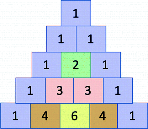
• 2. Write a function which implements Pascal’s triangle for a specified number of rows. Pascals triangle is a triangle of the binomial coefficients. The values held in the triangle are generated as follows: In row 0 (the topmost row), there is a unique nonzero entry 1. Each entry of each subsequent row is constructed by adding the number above and to the left with the number above and to the right, treating blank entries as 0. For example, the initial number in the first (or any other) row is 1 (the sum of 0 and 1), whereas the numbers 1 and 3 in the third row are added together to generate the number 4 in the fourth row. An example of Pascals triangle for 4 rows is given below:

  

For example, your function might be called pascals_traingle() in which case the following application illustrates how you might use it:

The output from this might be: