Axis

Petty, Brent G.

doi:10.1007/978-1-4939-2413-4_2

Brent G. Petty M.D.²

3880 Accesses

Abstract

The term “axis” as related to electrocardiograms usually means the QRS axis, but the P wave and the T wave axis can also be determined. The axis is the general direction of the electrical event in question, which is atrial depolarization (P waves), ventricular depolarization (QRS complexes), and ventricular repolarization (T waves). Axis is not a vector—axis only has direction, while a vector has both direction and amplitude. The normal direction of all the axes is inferior and left, between 0° and +90°. Changes in the direction of each axis can be meaningful in identifying the presence or progression of cardiac diseases in patients.

Access provided by Autonomous University of Puebla. Download chapter PDF

Keywords

The electrical axis of any electrocardiogram (EKG) waveform is the average direction of electrical activity. It is not a vector, because by definition a vector has both direction and amplitude, while axis has only direction. While the axis of any of the waves (P, QRS, T) can be determined, the term “axis,” unless otherwise specified, refers to the axis of the QRS complex.

One determines axis from the six limb leads only. These include the bipolar electrodes of Einthoven (I, II, and III) plus the augmented limb leads which can be thought of as bipolar electrodes with an intermediate orientation relative to leads I, II, and III. The six limb leads together constitute the “hexaxial reference system.” A bipolar electrode provides for a positive, negative, or isoelectric deflection on the recording paper, depending on the orientation of the electrode and the direction of the electrical activity (Fig. 2.1).

When electrical activity is going towards the positive pole of a bipolar electrode, a positive or upright deflection is recorded on the graph paper (see Fig. 2.1a). When electrical activity is going towards the negative pole, a negative or downward deflection is recorded (see Fig. 2.1b). When electrical activity is perpendicular to the lead, no deflection is recorded (see Fig. 2.1c). Because the heart is of more than one dimension and the direction of electrical activity is not always exactly in the same direction, no totally flat bipolar record is possible. The equivalent of the flat bipolar record in electrocardiography is the “isoelectric” lead, in which an equal upward and downward deflection is recorded (see Fig. 2.1d). It must be noted that the average direction of electrical activity in Fig. 2.1d is the same as in Fig. 2.1c, i.e., the average direction of electrical activity in both Fig. 2.1c and Fig. 2.1d is perpendicular to the orientation of the electrode. It should also be noted that the magnitude of the deflection is judged by the area above or below the deflection, not the mere height or depth of the deflection. Applying this concept to each of the limb leads means that if the net deflection (positive area vs. negative area) of the wave is positive, the axis is on the positive side of the perpendicular to that lead.

The six limb leads are arranged such that their intersections equally divide the circle of the frontal plane into 30° sectors (Fig. 2.2). The positive side of each lead is labelled with the lead’s identifier. As related to the expression of axis, horizontal towards the patient’s left is arbitrarily designated as 0°, with positive extending downward (clockwise) and negative extending upward (counterclockwise) from left horizontal. Whenever axis is reported, the report must include either “+” or “−,” except for 0° and 180°. A normal axis is between 0° and +90°, although some authors believe that the normal axis can actually extend as far to the left as −30°. Right axis deviation (RAD) is between +90° and 180°, left axis deviation (LAD) is between 0° and −90°, and either “extreme” right axis or “extreme” LAD is between 180° and +270°, or −90° and 180°, respectively.

With these fundamental concepts in mind, determination of axis can be easy and quick. There are three steps in determining axis (Table 2.1).

Table 2.1 Steps in determining electrical axis

Full size table

Step One: Examine leads I and aVF and see if the QRS deflections are net positive, net negative, or isoelectric. With this information, one can immediately determine the axis or, more usually, in which quadrant the axis is located—normal axis, RAD, LAD, or extreme axis deviation (Table 2.2). This is just a quick application of the positive vs. negative net deflection concept in the horizontal and vertical limb leads (I and aVF, respectively). If either I or aVF are isoelectric, then the axis is perpendicular to that lead and in the direction dictated by the other lead. Specifically, if I is isoelectric and aVF is positive, the axis is +90°. If aVF is isoelectric and I is positive, the axis is 0°. If I is isoelectric and aVF is negative, the axis is −90°. If aVF is isoelectric and I is negative, the axis is 180°.

Table 2.2 Determining the quadrant of the axis

Full size table

Step Two: If I and aVF show that the axis is in a quadrant, look further for an isoelectric lead. Again, this is the bipolar (limb) lead with equal area deflected above and below the baseline. If there is an isoelectric lead, the axis is perpendicular to that lead in the quadrant determined in the first step. An isoelectric lead is not sought before quadrant determination because the axis could be in either direction perpendicular to the isoelectric lead, and observing the other leads becomes necessary to reveal which direction is correct. The leads to examine for an isoelectric lead depend on which quadrant the axis is in; they are the leads whose perpendiculars trisect the quadrant the axis is in, based on Step One. If the axis is in either the normal or extreme axis quadrants, the trisecting perpendiculars are those of leads III and aVL. With either right or LAD, the trisecting perpendiculars are those of leads II and aVR. If one of these trisecting leads is isoelectric, the axis is perpendicular to that lead in the correct quadrant.

Step Three: If there is not an isoelectric lead, then one interpolates. Interpolation is within a 30° sector between two perpendiculars to leads. The correct 30° sector is determined by the net deflection of the waves in the limb leads (Table 2.3). This means that the leads closest to isoelectric are determined, and the relative positivity or negativity of the leads is examined to assess how close to isoelectric those leads are. The closer the lead is to isoelectric, the closer the axis is to the perpendicular of that lead. There should be no more than 5–15° interobserver or intraobserver variability in reading axis, and axis is conventionally reported by humans to the nearest 5° (computers are programmed to report axis to the nearest 1°).

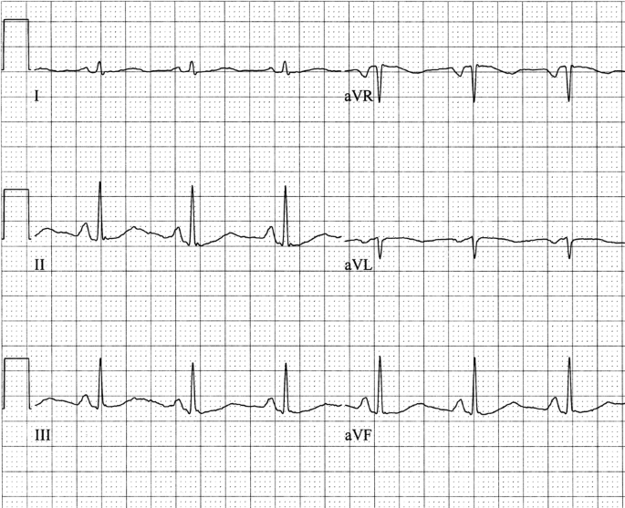
Table 2.3 Sectors of interpolation according to limb lead deflection

Full size table

Some examples should be helpful in illustrating these concepts. Consider Fig. 2.3 in stepwise fashion regarding the determination of the QRS axis. First, look at leads I and aVF. Both have net positive QRS complexes, so you know immediately that the axis is in the normal quadrant, somewhere between 0 and +90°. Next, look for an isoelectric lead, and because the axis is in the normal quadrant we examine leads III and aVL. The QRS complexes in lead aVL have equal areas under the upward and above the downward deflections, i.e., lead aVL is isoelectric. Therefore, the QRS axis is perpendicular to the orientation of lead aVL and is in the normal quadrant, or +60°.

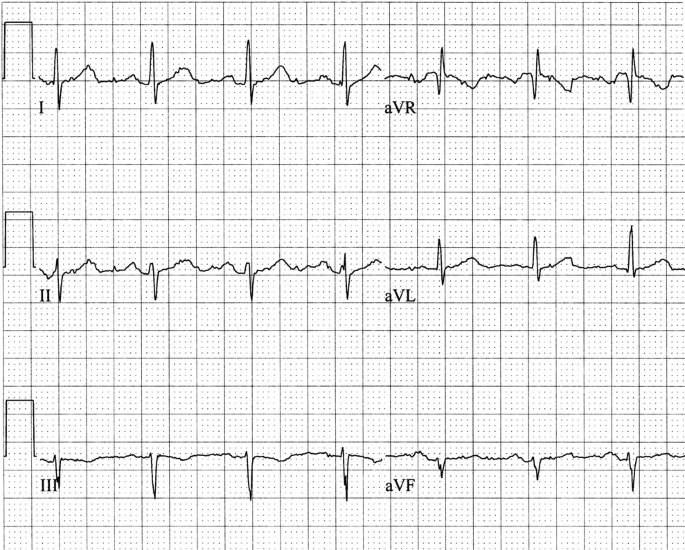
Now turn to the tracing in Fig. 2.4. First, look at leads I and aVF. Lead I is net positive, but lead aVF is net negative, so you know that the axis is in the LAD quadrant, somewhere between 0° and −90°. Next, look for an isoelectric lead. Because the axis is in the LAD quadrant, look at leads II and aVR. The QRS complexes in lead II are isoelectric, so the QRS axis is perpendicular to lead II in the LAD quadrant, or −30°.

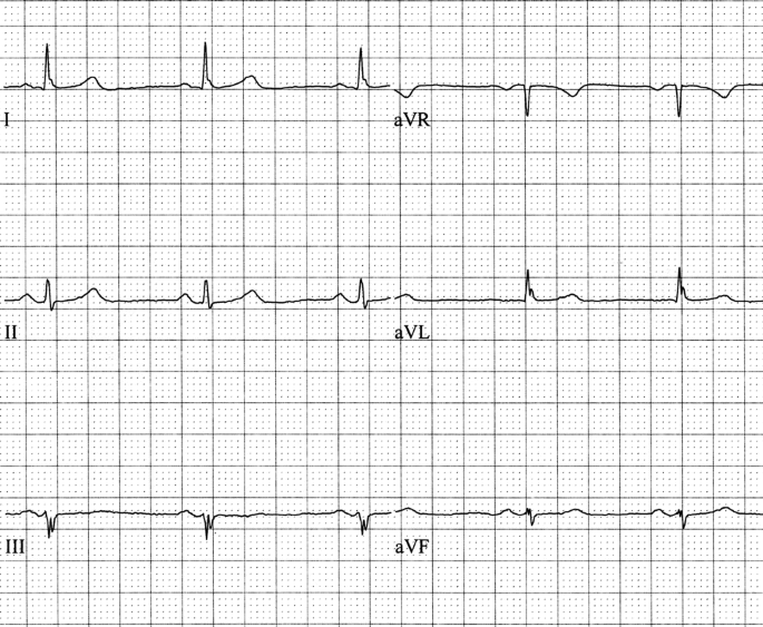
Now try Fig. 2.5. Lead I is net negative and aVF is net positive, so the axis is in the RAD quadrant, somewhere between +90° and 180°. Because the axis is in the RAD quadrant, look at leads II and aVR for the isoelectric lead. The QRS complexes are isoelectric in aVR, so the axis is perpendicular to that lead in the RAD quadrant, or +120°.

Now consider Fig. 2.6. First, look at leads I and aVF. Both leads I and aVF are positive. Therefore, the axis is in the normal quadrant. For that reason, we look at leads III and aVL for an isoelectric lead. It appears that III is isoelectric, so the axis is perpendicular to lead III in the normal quadrant, or +30°.

Next, consider the record in Fig. 2.7. In examining leads I and aVF, one finds that lead aVF is isoelectric, so the axis does not fall within a quadrant, but rather is on the horizontal. Because lead I is positive, the axis must be 0° (rather than 180°, which would require lead I to be negative). In Fig. 2.8, I is isoelectric and aVF is positive, so the axis is +90°.

All of the previous tracings have had an isoelectric lead, which makes determining the axis quite simple. Now let us turn to Fig. 2.9. Both leads I and aVF are net positive, so we know that the axis is in the normal quadrant. Next, we look for an isoelectric lead, and because the axis is in the normal quadrant we look at leads III and aVL. Neither of those is isoelectric, however, so we must proceed to Step Three, which is to interpolate. Considering leads I, III, aVL, and aVF, the leads closest to isoelectric are leads III and aVL. If III were isoelectric, the axis would be +30°, but since III is net positive, the axis must be on the positive side of III, or to the right of (more positive than) +30°. If aVL were isoelectric, the axis would be +60, but because aVL is net positive, the axis must be on the positive side of aVL, or to the left of (less positive than) +60°. Thus, the axis is between +30° and +60°. Carefully comparing the relative positive and negative deflections of leads III and aVL reveals that the QRS complexes in the two leads are very similar. Therefore, the axis is midway between the lines perpendicular to these two leads, or +45°.

Another example of interpolation is given in Fig. 2.10. Lead I is net positive but aVF is negative, so the axis is in the LAD quadrant. Examining leads II and aVR shows that neither is isoelectric, but lead II is closest to isoelectric. If lead II were isoelectric, the axis would be −30°, but since lead II is positive, the axis must be on the positive side of II, or to the right of (less negative than) −30°. Because lead aVF is negative, the axis must be to the left of (more negative than) 0°. Therefore, the axis is somewhere between 0° and −30°. Because lead II is closer to isoelectric than lead aVF, the axis is closer to −30° than 0°, or about −20°. Keep in mind that the closer a lead is to isoelectric, the closer the axis is to the perpendicular of that lead.

Rarely it appears that several or all of the bipolar leads have isoelectric QRS complexes (Fig. 2.11). In this case, the axis is “indeterminate” because no axis value is consistent with all of the observed QRS configurations. The pathological significance of an indeterminate axis is unclear, but it probably represents a normal variant.

The method presented above to determine axis is not the only method that can be used, but it is the method which I find easiest. With just a little practice and familiarity with the orientation of the leads, determining the axis by the method shown here can be done very rapidly.

Electrical axis is important because deviations in the axis are associated with various conditions (Table 2.4). Furthermore, a change in a patient’s axis may give a hint into the nature of the patient’s problem. For example, consider a patient with chest pain and shortness of breath who has a previous EKG showing an axis of +10° and now has an EKG with an axis of +85° but no other changes in waveform and a normal chest X-ray. In both EKGs the axis is normal, but the significant rightward shift suggests right ventricular stress and should raise the suspicion of pulmonary embolism. Other acute pulmonary disease, such as pneumothorax, pneumonia, or hydrothorax, could conceivably shift the axis rightward as well.

Table 2.4 Conditions associated with axis deviation

Full size table

As mentioned at the outset, the P wave axis and T wave axis can also be determined by applying the same principles explained above for the QRS axis. The P wave axis is usually in the normal quadrant, and the T wave axis should be no more than 60–70° different than the QRS axis. When the T wave axis deviates further from the QRS axis, an abnormality (e.g., ischemia, left ventricular strain, or metabolic disturbance) is present.

A special situation exists when determining the axis if the QRS duration is 0.12 s or longer. This is the situation with bundle branch blocks (see Chap. 5). Because of the distortion of conduction induced by the bundle branch block, it is proper to use only the first 0.08 s of the QRS complex to determine the electrical axis. The last portion of the QRS complex, the so-called terminal force, is a reflection of the conduction abnormality induced by the bundle branch block. Using the first 0.08 s is a method of at least partially correcting for the terminal forces, reducing the distortion induced by the bundle branch block. The terminal forces are especially misleading in the case of right bundle branch block and less so in left bundle branch block. An example of using the first 0.08 s for determining axis in the presence of a bundle branch block is given in Fig. 2.12.

Exercise Tracings

Determine the electrical axis for the QRS complexes in the following examples. In each case, only the limb leads are provided. Your answer should be within 10° of mine, but hopefully closer!