
Abstract
This chapter is devoted to the study of mixed boundary value problems in electromagnetic scattering theory. Mixed boundary value problems typically model scattering by objects that are coated with a thin layer of material on part of the boundary. We shall consider here two main problems: (1) the scattering by a perfect conductor that is partially coated with a thin dielectric layer and (2) scattering by an orthotropic dielectric that is partially coated with a thin layer of highly conducting material. The first problem leads to an exterior mixed boundary value problem for the Helmholtz equation where on the coated part of the boundary the total field satisfies an impedance boundary condition and on the remaining part of the boundary the total field vanishes, while the second problem leads to a transmission problem with mixed transmission-conducting boundary conditions. In this chapter we shall present a mathematical analysis of these two mixed boundary value problems.
Access provided by Autonomous University of Puebla. Download chapter PDF
Keywords
- Mixed Boundary Value Problem
- Impedance Boundary Condition
- Perfect Conductor
- Herglotz Wave Function
- Linear Sampling Method
These keywords were added by machine and not by the authors. This process is experimental and the keywords may be updated as the learning algorithm improves.
This chapter is devoted to the study of mixed boundary value problems in electromagnetic scattering theory. Mixed boundary value problems typically model scattering by objects that are coated with a thin layer of material on part of the boundary. We shall consider here two main problems: (1) the scattering by a perfect conductor that is partially coated with a thin dielectric layer and (2) scattering by an orthotropic dielectric that is partially coated with a thin layer of highly conducting material. The first problem leads to an exterior mixed boundary value problem for the Helmholtz equation where on the coated part of the boundary the total field satisfies an impedance boundary condition and on the remaining part of the boundary the total field vanishes, while the second problem leads to a transmission problem with mixed transmission-conducting boundary conditions. In this chapter we shall present a mathematical analysis of these two mixed boundary value problems.
In the study of inverse problems for partially coated obstacles, it is important to mentioned that, in general, it is not known a priori whether or not the scattering object is coated and, if so, what the extent of the coating is. Hence the linear sampling method becomes the method of choice for solving inverse problems for mixed boundary value problems since it does not make use of the physical properties of the scattering object. In addition to the reconstruction of the shape of the scatterer, a main question in this chapter will be to determine whether the obstacle is coated and if so what the electrical properties of the coating are. In particular, we will show that the solution of the far-field equation that was used to determine the shape of the scatterer by means of the linear sampling method can also be used in conjunction with a variational method to determine the maximum value of the surface impedance of the coated portion in the case of partially coated perfect conductors and of the surface conductivity in the case of partially coated dielectrics.
Finally, we will extend the linear sampling method to the scattering problem by very thin objects, referred to as cracks, which are modeled by open arcs in \({\mathbb{R}}^{2}\).
8.1 Scattering by a Partially Coated Perfect Conductor
We consider the scattering of an electromagnetic time-harmonic plane wave by a perfectly conducting infinite cylinder in \({\mathbb{R}}^{3}\) that is partially coated with a thin dielectric material. In particular, the total electromagnetic field on the uncoated part of the boundary satisfies the perfect conducting boundary condition, that is, the tangential component of the electric field is zero, whereas the boundary condition on the coated part is described by an impedance boundary condition [79].
More precisely, let D denote the cross section of the infinitely long cylinder and assume that \(D \subset {\mathbb{R}}^{2}\) is an open bounded region with C 2 boundary ∂D such that \({\mathbb{R}}^{2}\setminus \bar{D}\) is connected. The boundary ∂D has the dissection \(\partial D = \overline{\partial D}_{D} \cup \overline{\partial D}_{I}\), where ∂D D and ∂D I are disjoint, relatively open subsets (possibly disconnected) of ∂D. Let ν denote the unit outward normal to ∂D, and assume that the surface impedance \(\lambda \in C(\overline{\partial D}_{I})\) satisfies λ(x) ≥ λ 0 > 0 for x ∈ ∂D I . Then the total field u = u s + u i, given as the sum of the unknown scattered field u s and the known incident field u i, satisfies
where k > 0 is the wave number and u s satisfies the Sommerfeld radiation condition
uniformly in \(\hat{x} = x/\vert x\vert \) with r = | x |. Note that here again the incident field u i is usually an entire solution of the Helmholtz equation. In particular, in the case of incident plane waves, we have u i(x) = e ikx⋅ d, where d: = (cos \(\phi\), sin \(\phi\)) is the incident direction and \(x = (x_{1},\,x_{2}) \in {\mathbb{R}}^{2}\).
Due to the boundary condition, the preceding exterior mixed boundary value problem may not have a solution in \({C}^{2}({\mathbb{R}}^{2}\setminus \bar{D}) \cap {C}^{1}(\mathbb{R}\setminus D)\), even for incident plane waves and analytic boundary. In particular, the solution fails to be differentiable at the boundary points of \(\overline{\partial D}_{D} \cap \overline{\partial D}_{I}\). Therefore, looking for a weak solution in the case of mixed boundary value problems is very natural.
To define a weak solution to the mixed boundary value problem in the energy space H 1(D), we need to understand the respective trace spaces on parts of the boundary. To this end, we now present a brief discussion of Sobolev spaces on open arcs. The classic reference for such spaces is [124]. For a systematic treatment of these spaces, we refer the reader to [127].
Let ∂D 0 ⊆ ∂D be an open subset of the boundary. We define
i.e., the space of restrictions to ∂D 0 of functions in \({H}^{\frac{1} {2}}(\partial D)\), and define
where supp u is the essential support of u, i.e., the largest relatively closed subset of ∂D such that u = 0 almost everywhere on ∂D ∖ supp u. We can identify \(\tilde{{H}}^{\frac{1} {2}}(\partial D_{0})\) with a trace space of \(H_{0}^{1}(D,\partial D\setminus \overline{\partial D}_{0})\), where
A very important property of \(\tilde{{H}}^{\frac{1} {2}}(\partial D_{0})\) is that the extension by zero of \(u \in \tilde{ {H}}^{\frac{1} {2}}(\partial D_{0})\) to the whole ∂D is in \({H}^{\frac{1} {2}}(\partial D)\) and the zero extension operator is bounded from \(\tilde{{H}}^{\frac{1} {2}}(\partial D_{0})\) to \({H}^{\frac{1} {2}}(\partial D)\). It can also be shown (cf. Theorem A4 in [127]) that there exists a bounded extension operator \(\tau: {H}^{\frac{1} {2}}(\partial D_{0}) \rightarrow {H}^{\frac{1} {2}}(\partial D)\). In other words, for any \(u \in {H}^{\frac{1} {2}}(\partial D_{0})\) there exists an extension \(\tau u \in {H}^{\frac{1} {2}}(\partial D)\) such that
with C independent of u, where
Example 8.1.
Consider the step function
Using the definition of Sobolev spaces in terms of the Fourier coefficients (Sect. 1.4) it is easy to show that the step function is not in \({H}^{\frac{1} {2}}[0,\,2\pi]\). In particular, the Fourier coefficients of u are a 2k = 0 and a 2k+1 = 1∕(i(2k + 1)π), whence
Now consider the unit circle \(\partial \varOmega =\{ x \in {\mathbb{R}}^{2}:\; x = (\sin \,t,\;\cos \,t),\;t \in [0,\,2\pi]\}\), and denote by \(\partial \varOmega _{0} =\{ x \in {\mathbb{R}}^{2}:\; x = (\sin \,t,\;\cos \,t),\;t \in [0,\,\pi]\}\) the upper half-circle. Let \(v: \partial \varOmega _{0} \rightarrow \mathbb{R}\) be the constant function v = 1. By definition, \(v \in {H}^{\frac{1} {2}}(\partial \varOmega _{0})\) since it is the restriction to ∂ Ω 0 of the constant function 1 defined on the whole circle ∂ Ω that is in \({H}^{\frac{1} {2}}(\partial \varOmega)\). But \(v\notin \tilde{{H}}^{\frac{1} {2}}(\partial \varOmega _{0})\) since its extension by zero to the whole circle is not in \({H}^{\frac{1} {2}}(\partial \varOmega)\) [note that the extension \(\tilde{v}(\sin \,t,\,\cos \,t)\) is a step function and from the preceding discussion is not in \({H}^{\frac{1} {2}}[0,\,2\pi]\)].
The foregoing example shows that if \(u \in \tilde{ {H}}^{\frac{1} {2}}(\partial D_{0})\), then it has a certain behavior at the boundary of ∂D 0 in ∂D. A better insight into this behavior is given in [124]. In particular, the space \(\tilde{{H}}^{\frac{1} {2}}(\partial D_{0})\) coincides with the space
where r is the polar radius.
Both \({H}^{\frac{1} {2}}(\partial D_{0})\) and \(\tilde{{H}}^{\frac{1} {2}}(\partial D_{0})\) are Hilbert spaces when equipped with the restriction of the inner product of \({H}^{\frac{1} {2}}(\partial D)\). Hence, we can define the corresponding dual spaces
and
with respect to the duality pairing explained in what follows.
A bounded linear functional \(F \in {H}^{-\frac{1} {2}}(\partial D_{0})\) can in fact be seen as the restriction to ∂D 0 of some \(\tilde{F} \in {H}^{-\frac{1} {2}}(\partial D)\) in the following sense: if \(\tilde{u} \in {H}^{\frac{1} {2}}(\partial D)\) denotes the extension by zero of \(u \in \tilde{ {H}}^{\frac{1} {2}}(\partial D_{0})\), then the restriction \(F:=\tilde{ F}\vert _{\partial D_{0}}\) is defined by
With the preceding understanding, to unify the notations, we identify
and
where \(\left< \cdot,\cdot \right>\) denotes the duality pairing between the denoted spaces and \(\tilde{u} \in {H}^{\frac{1} {2}}(\partial D)\) is the extension by zero of \(u \in \tilde{ {H}}^{\frac{1} {2}}(\partial D_{0})\).
For a bounded linear functional \(F \in {H}^{-\frac{1} {2}}(\partial D)\), we define supp F to be the largest relatively closed subset of ∂D such that the restriction of F to ∂D ∖ supp F is zero. Similarly, for \(\tilde{{H}}^{\frac{1} {2}}(\partial D_{0})\) we can now write
Therefore, the extension by zero \(\tilde{v} \in {H}^{-\frac{1} {2}}(\partial D)\) of \(v \in \tilde{ {H}}^{-\frac{1} {2}}(\partial D_{0})\) is well defined and
where \(u \in {H}^{\frac{1} {2}}(\partial D)\).
We can now formulate the following mixed boundary value problems:
Exterior mixed boundary value problem: Let \(f \in {H}^{\frac{1} {2}}(\partial D_{D})\) and \(h \in {H}^{-\frac{1} {2}}(\partial D_{I})\). Find a function \(u \in H_{loc}^{1}({\mathbb{R}}^{2}\setminus \bar{D})\) such that
Note that the scattering problem for a partially coated perfect conductor (8.1)–(8.4) is a special case of (8.6)–(8.9). In particular, the scattered field u s satisfies (8.6)–(8.9) with \(f:= -{u}^{i}\vert _{\partial D_{D}}\) and \(h:= -\partial {u}^{i}/\partial \nu - i\lambda {u}^{i}\vert _{\partial D_{I}}\).
For later use we also consider the corresponding interior mixed boundary value problem.
Interior mixed boundary value problem: Let \(f \in {H}^{\frac{1} {2}}(\partial D_{D})\) and \(h \in {H}^{-\frac{1} {2}}(\partial D_{I})\). Find a function u ∈ H 1(D) such that
Theorem 8.2.
Assume that ∂D I ≠ ∅ and λ ≠ 0. Then the interior mixed boundary value problem (8.10) – (8.12) has at most one solution in H 1 (D).
Proof.
Let u be a solution to (8.10)–(8.12), with f ≡ 0 and h ≡ 0. Then an application of Green’s first identity in D yields
and making use of homogeneous boundary condition we obtain
Since λ is a real-valued function and λ(x) ≥ λ 0 > 0, taking the imaginary part of (8.14) we conclude that \(u\vert _{\partial D_{I}} \equiv 0\) as a function in \({H}^{\frac{1} {2}}(\partial D_{I})\), and consequently \(\partial u/\partial \nu \vert _{\partial D_{I}} \equiv 0\) as a function in \({H}^{-\frac{1} {2}}(\partial D_{I})\).
Now let \(\varOmega _{\rho}\) be a disk of radius ρ with center on ∂D I such that \(\bar{\varOmega}_{\rho} \cap \partial D_{D} = \emptyset \), and define v = u in \(D \cap \varOmega _{\rho}\), v = 0 in \(({\mathbb{R}}^{2}\setminus \bar{D}) \cap \varOmega _{\rho}\). Then applying Green’s first identity in each of these domains to v and a test function \(\overline{\varphi} \in C_{0}^{\infty}(\varOmega _{\rho})\) we see that v is a weak solution to the Helmholtz equation in Ω ρ . Thus v is a real-analytic solution in Ω ρ . We can now conclude that u ≡ 0 in Ω ρ , and thus u ≡ 0 in D.
Theorem 8.3.
The exterior mixed boundary value problem (8.6) – (8.9) has at most one solution in \(H_{loc}^{1}({\mathbb{R}}^{2}\setminus \bar{D})\) .
Proof.
The proof of the theorem is essentially the same as the proof of Theorem 3.3.
Theorem 8.4.
Assume that ∂D I ≠ ∅ and λ ≠ 0. Then the interior mixed boundary value problem (8.10) – (8.12) has a solution that satisfies the estimate
with C a positive constant independent of f and h.
Proof.
To prove the theorem, we use the variational approach developed in Sect. 5.3. (For a solution procedure based on integral equations of the first kind we refer the reader to [23]). Let \(\tilde{f} \in {H}^{\frac{1} {2}}(\partial D)\) be the extension of the Dirichlet data \(f \in {H}^{\frac{1} {2}}(\partial D_{D})\) that satisfies \(\|\tilde{f}\|_{{ H}^{\frac{1} {2}}(\partial D)} \leq C\|f\|_{{ H}^{\frac{1} {2}}(\partial D_{D})}\) given by (8.5), and let \(u_{0} \in {H}^{1}(D)\) be such that \(u_{0} =\tilde{ f}\) on ∂D and \(\|u_{0}\|_{{H}^{1}(D)} \leq C\|\tilde{f}\|_{{ H}^{\frac{1} {2}}(\partial D)}\). In particular, we may choose \(u_{0}\) to be a solution of Δ u 0 = 0 (Example 5.15). Defining the Sobolev space \(H_{0}^{1}(D,\partial D_{D})\) by
equipped with the norm induced by H 1(D), we observe that \(w = u - u_{0} \in H_{0}^{1}(D,\partial D_{D})\), where u ∈ H 1(D) is a solution to (8.10)–(8.12). Furthermore, w satisfies
and
where \(\tilde{h} \in {H}^{-\frac{1} {2}}(\partial D_{I})\) is given by
Multiplying (8.16) by a test function \(\overline{\varphi} \in H_{0}^{1}(D,\partial D_{D})\) and using Green’s first identity together with the boundary condition (8.17) we can write (8.10)–(8.12) in the following equivalent variational form: find u ∈ H 1 (D) such that \(w = u - u_{0} \in H_{0}^{1}(D,\partial D_{D})\) and
where the sesquilinear form \(a\left(\cdot,\,\cdot \right): H_{0}^{1}(D,\partial D_{D}) \times H_{0}^{1}(D,\partial D_{D}) \rightarrow \mathbb{C}\) is defined by
and the conjugate linear functional \(L: H_{0}^{1}(D,\partial D_{D}) \rightarrow \mathbb{C}\) is defined by
where the integral over ∂D I is interpreted as the duality pairing between \(\tilde{h} \in {H}^{-\frac{1} {2}}(\partial D_{I})\) and \(\bar{\varphi}\in \tilde{ {H}}^{\frac{1} {2}}(\partial D_{I})\) [note that \(\bar{\varphi}\in \tilde{ {H}}^{\frac{1} {2}}(\partial D_{I})\) since \(\tilde{{H}}^{\frac{1} {2}}(\partial D_{I})\) is the trace space of \(H_{0}^{1}(D,\partial D_{D})\)].
Next we write a(⋅, ⋅) as the sum of two terms \(a(\cdot,\,\cdot) = a_{1}(\cdot,\,\cdot) + a_{2}(\cdot,\,\cdot)\), where
and
From the Cauchy–Schwarz inequality and the trace Theorem 1.38, since λ is a bounded function on ∂D I , we have that
and
Hence a 1(⋅, ⋅) and a 2(⋅, ⋅) are bounded sesquilinear forms.
Furthermore, noting that \(\varphi = 0\) on ∂D D , we have that
Therefore, from the previous estimates and the trace Theorems 1.38 and 5.7 we have that
\(\mbox{ for all}\;\varphi \in H_{0}^{1}(D,\partial D_{0})\), which shows that L is a bounded conjugate linear functional and
with the constant C > 0 independent of f and h.
Next, since λ is real, we can write
whence a 1(⋅, ⋅) is strictly coercive.
Therefore, from the Lax–Milgram lemma there exists a bijective bounded linear operator \(A: H_{0}^{1}(D,\partial D_{D}) \rightarrow H_{0}^{1}(D,\partial D_{D})\) with bounded inverse such that \(\left(Aw,\varphi \right) = a_{1}(w,\,\varphi)\) for all w and \(\varphi\) in \(H_{0}^{1}(D,\partial D_{D})\). Finally, due to the compact embedding of H 1(D) into L 2(D), there exists a compact bounded linear operator \(B: H_{0}^{1}(D,\partial D_{D}) \rightarrow H_{0}^{1}(D,\partial D_{D})\) such that \(\left(Bw,\varphi \right) = a_{2}(w,\,\varphi)\) for all w and \(\varphi\) in \(H_{0}^{1}(D,\partial D_{D})\) (Example 5.17). Therefore, from Theorems 5.16 and 8.2 we obtain the existence of a unique solution to (8.18) and, consequently, to the interior mixed boundary value problem (8.10)–(8.12). The a priori estimate (8.15) follows from (8.19).
Now let us consider an open disk Ω R of radius R centered at the origin and containing \(\bar{D}\).
Theorem 8.5.
The exterior mixed boundary value problem (8.6) – (8.9) has a solution that satisfies the estimate
with C a positive constant independent of f and h but depending on R.
Proof.
First, exactly in the same way as in Example 5.23, we can show that the exterior mixed boundary value problem (8.6)–(8.9) is equivalent to the following problem:
where T is the Dirichlet-to-Neumann map. If \(\tilde{f} \in {H}^{\frac{1} {2}}(\partial D)\) is the extension of \(f \in {H}^{\frac{1} {2}}(\partial D_{D})\) that satisfies (8.5) with ∂D 0 replaced by ∂D D , then we construct \(u_{0} \in {H}^{1}(\varOmega _{R}\setminus \bar{D})\) such that \(u_{0} =\tilde{ f}\) on ∂D, u = 0 on ∂ Ω R , and Δ u 0 = 0 in \(\varOmega _{R}\setminus \bar{D}\) (Example 5.15). Then, for every solution u to (8.21)–(8.24), w = u − u 0 is in the Sobolev space \(H_{0}^{1}(\varOmega _{R}\setminus \bar{D},\partial D_{D})\) defined by
and satisfies the variational equation
Making use of Theorem 5.22, the assertion of the theorem can now be proven in the same way as in Theorem 8.4.
Remark 8.6.
In the case where either ∂D I = ∅ (this case corresponds to the Dirichlet boundary value problem) or λ = 0, the corresponding interior problem may not be uniquely solvable. If nonuniqueness occurs, then k 2 is said to be an eigenvalue of the corresponding boundary value problem. In these cases, Theorem 8.4 holds true under the assumption that k 2 is not an eigenvalue of the corresponding boundary value problem.
Remark 8.7.
Due to the change in the boundary conditions, the solution to the mixed boundary value problems (8.6)–(8.9) and (8.10)–(8.12) has a singular behavior near the boundary points in \(\overline{\partial D}_{D} \cup \overline{\partial D}_{N}\). In particular, even for C ∞ boundary ∂D and analytic incident waves u i, the solution in general is not in \(H_{loc}^{2}({\mathbb{R}}^{2}\setminus \bar{D})\). More precisely, the most singular term of the solution behaves like \(O({r}^{\frac{1} {2}})\), where (r, \(\phi\)) denotes the local polar coordinates centered at the boundary points in \(\overline{\partial D}_{D} \cup \overline{\partial D}_{N}\) [65]. This is important to take into consideration when finite element methods are used.
8.2 Inverse Scattering Problem for Partially Coated Perfect Conductor
We now consider time-harmonic incident fields given by \({u}^{i}(x) = {e}^{ikx\cdot d}\) with incident direction d: = (cos \(\phi\), sin \(\phi\)) and \(x = (x_{1},\,x_{2}) \in {\mathbb{R}}^{2}\). The corresponding scattered field \({u}^{s} = {u}^{s}(\cdot,\,\phi)\), which satisfies (8.1)–(8.4), depends also on the incident angle \(\phi\) and has the asymptotic behavior (4.5). The far-field pattern u ∞ (θ, \(\phi\)), \(\theta \in [0,\,2\pi]\) of the scattered field defines the far-field operator \(F: {L}^{2}[0,\,2\pi] \rightarrow {L}^{2}[0,\,2\pi]\) corresponding to the scattering problem (8.1)–(8.4) by
The inverse scattering problem for a partially coated perfect conductor is given the far-field pattern \(u_{\infty}(\theta,\phi)\) for \(\theta \in [0,\,2\pi]\) and \(\phi \in [0,\,2\pi]\) determines both D and λ = λ(x) for x ∈ ∂D I .
In the same way as in the proof of Theorem 4.3, using Theorem 8.2 we can show the following result.
Theorem 8.8.
Assume that ∂D I ≠ ∅ and λ ≠ 0. Then the far-field operator corresponding to the scattering problem (8.1) – (8.4) is injective with a dense range.
Remark 8.9.
If ∂D I = ∅ or λ = 0, then all the following results about the far-field operator and the determination of D remain valid assuming the uniqueness for the corresponding interior boundary value problem. Note that the case of ∂D I = ∅ corresponds to the scattering problem for a perfect conductor.
Concerning the unique determination of D, the following theorem can be proved in the same way as Theorem 4.5. The only change needed in the proof is that we can always choose the point x ∗ such that either \(\varOmega _{\epsilon}({x}^{{\ast}}) \cap \partial D_{1} \subset \partial D_{1D}\) or \(\varOmega _{\epsilon}({x}^{{\ast}}) \cap \partial D_{1} \subset \partial D_{1I}\) for some small disk \(\varOmega _{\epsilon}({x}^{{\ast}})\) centered at x ∗ of radius \(\epsilon\) and satisfying \(\varOmega _{\epsilon}({x}^{{\ast}}) \cap \bar{D}_{2} = \emptyset \), whence one uses either the Dirichlet condition or impedance condition at x ∗ to arrive at a contraction.
Theorem 8.10.
Assume that D 1 and D 2 are two partially coated scattering obstacles with corresponding surface impedances λ 1 and λ 2 such that for a fixed wave number the far-field patterns for both scatterers coincide for all incident angles \(\phi\). Then D 1 = D 2 .
Theorem 8.11.
Assume that D 1 and D 2 are two partially coated scattering obstacles with corresponding surface impedances λ 1 and λ 2 such that for a fixed wave number the far-field patterns coincide for all incident angles ϕ. Then D 1 = D 2 and λ 1 = λ 2 .
Proof.
By Theorem 8.10, we first have that D 1 = D 2 = D. Then, following the proof of Theorem 4.7 we can prove that the total fields u 1 and u 2 corresponding to λ 1 and λ 2 coincide in \({\mathbb{R}}^{2}\setminus \bar{D}\), whence u 1 = u 2 and \(\partial u_{1}/\partial \nu = \partial u_{2}/\partial \nu\) on ∂D. From the boundary condition we have
for j = 1, 2. First we observe that \(\partial D_{D_{1}} \cap \partial D_{D_{2}} = \emptyset \), because otherwise \(u_{1} = \partial u_{1}/\partial \nu = 0\) on an open arc Γ ⊂ ∂D and a contradiction can be obtained as in the proof of Theorem 4.7. Hence \(\partial D_{I_{1}} = \partial D_{I_{2}} = \partial D_{I}\). Next,
and again one can conclude that λ 1 = λ 2, as in Theorem 4.7.
Having proved the uniqueness results, we now turn our attention to finding an approximation to D and λ. Our reconstruction algorithm is based on solving the far-field equation
where \(\varPhi _{\infty}(\hat{x},z)\) is the far-field pattern of the fundamental solution (Sect. 4.3). The far-field equation can be written as
where \(B: {H}^{\frac{1} {2}}(\partial D_{D}) \times {H}^{-\frac{1} {2}}(\partial D_{I}) \rightarrow {L}^{2}[0,\,2\pi]\) maps the boundary data (f, h) to the far-field pattern u ∞ of the radiating solution u to the corresponding exterior mixed boundary value problem (8.6)–(8.9), and \(H: {L}^{2}[0,\,2\pi] \rightarrow {H}^{\frac{1} {2}}(\partial D_{D}) \times {H}^{-\frac{1} {2}}(\partial D_{I})\) is defined by
with v g being the Herglotz wave function with kernel g.
Lemma 8.12.
Any pair \((f,h) \in {H}^{\frac{1} {2}}(\partial D_{D}) \times {H}^{-\frac{1} {2}}(\partial D_{I})\) can be approximated in \({H}^{\frac{1} {2}}(\partial D_{D}) \times {H}^{-\frac{1} {2}}(\partial D_{I})\) by Hg.
Proof.
Let u be the unique solution to (8.10)–(8.12) with boundary data (f, h). Then the result of this lemma is a consequence of Lemma 6.45 applied to this u and the trace Theorems 1.38 and 5.7.
Lemma 8.13.
The bounded linear operator \(B: {H}^{\frac{1} {2}}(\partial D_{D}) \times {H}^{-\frac{1} {2}}(\partial D_{I}) \rightarrow {L}^{2}[0,\,2\pi]\) is compact and injective and has a dense range.
Proof.
The proof proceeds as the proof of Theorem 4.8 making use of Theorems 8.5 and 8.8.
Using Lemmas 8.12 and 8.13 we can now prove in a similar way as in Theorem 4.11 the following result.
Theorem 8.14.
Assume that ∂D I ≠ ∅ and λ ≠ 0. Let u ∞ be the far-field pattern corresponding to the scattering problem (8.1) – (8.4) with associated far-field operator F. Then the following statements hold:
-
1.
For z ∈ D and a given \(\epsilon > 0\) there exists a function \(g_{z}^{\epsilon} \in {L}^{2}[0,2\pi]\) such that
$$\displaystyle{\|Fg_{z}^{\epsilon} -\varPhi _{ \infty}(\cdot,z)\|_{{L}^{2}[0,2\pi]} <\epsilon}$$and the Herglotz wave function \(v_{g_{z}^{\epsilon}}\) with kernel \(g_{z}^{\epsilon}\) converges in H 1 (D) as \(\epsilon \rightarrow 0\).
-
2.
For z ∉ D and a given \(\epsilon > 0\) every function \(g_{z}^{\epsilon} \in {L}^{2}[0,2\pi]\) that satisfies
$$\displaystyle{\|Fg_{z}^{\epsilon} -\varPhi _{ \infty}(\cdot,z)\|_{{L}^{2}[0,2\pi]} <\epsilon}$$is such that
$$\displaystyle{\lim _{\epsilon \rightarrow 0}\|v_{g_{z}^{\epsilon}}\|_{{H}^{1}(D)} = \infty.}$$
An approximation to D can now be obtained as the set of points z, where \(\|g_{z}\|_{{L}^{2}[0,\,2\pi]}\) becomes large, with g z the approximate solution to the far-field equation given by Theorem 8.14. Note that the factorization method to characterize D from the range of (F ∗ F)1∕4 cannot be established for the scattering problem with mixed boundary conditions. Hence a rigorous justification of the linear sampling method similar to Theorem 7.39 for this case is still an open problem.
Having determined D, in a similar way as in Sect. 4.4, we can now use g z given by Theorem 8.14 to determine an approximation to the maximum value of λ. In particular, let u z be the unique solution to
where z ∈ D and λ ∈ C(∂D I ), λ(x) ≥ λ 0 > 0. From the proof of the first part of Theorem 8.14 the following result is valid.
Lemma 8.15.
Assume ∂D I ≠ ∅ and λ ≠ 0. Let \(\epsilon > 0\), z ∈ D, and let u z be the unique solution of (8.26)–(8.28). Then there exists a Herglotz wave function \(v_{g_{z}}\) with kernel \(g_{z} \in {L}^{2}[0,\,2\pi]\) such that
Moreover, there exists a positive constant C > 0 independent of \(\epsilon\) such that
Now define w z by
In particular,
interpreted in the sense of the trace theorem. Repeating the proof of Theorem 4.12 with minor changes accounting for the boundary conditions (8.32) we have the following result.
Lemma 8.16.
For every \(z_{1},z_{2} \in D\) we have that
where \(\gamma = {e}^{i\pi /4}/\sqrt{8\pi k}\) and J 0 is a Bessel function of order zero.
Assuming D is connected, consider a disk Ω r ⊂ D of radius r contained in D (Remark 4.13), and define
Lemma 8.17.
W is complete in \({L}^{2}(\partial D_{I})\) .
Proof.
Let \(\varphi\) be a function in \({L}^{2}(\partial D_{I})\) such that for every z ∈ Ω r
Using Theorem 8.4, let v ∈ H 1(D) be the unique solution of the interior mixed boundary value problem
Then for every z ∈ Ω r , using the boundary conditions and the integral representation formula, we have that
The unique continuation principle for solutions to the Helmholtz equation now implies that v(z) = 0 for all z ∈ D, whence from the trace theorem \(\varphi = 0\).
⊓⊔
Setting z = z 1 = z 2 in Lemma 8.16 we arrive at the following integral equation for the determination of λ:
or, noting that u z +Φ(⋅, z) = 0 on ∂D D ,
where u z is defined by (8.26)–(8.28). By Lemma 8.17, we see that the left-hand side of this equation is an injective compact integral operator with positive kernel defined on \({L}^{2}(\partial _{D})\). Using the Tikhonov regularization technique (cf. [68]) it is possible to determine λ by finding the regularized solution of (8.33) in L 2(∂D) (i.e., it is not necessary to know a priori the coated portion ∂D I ). Note that this integral equation has both noisy kernel and noisy right-hand side (recall from Lemma 8.15 that u z can be approximated by \(v_{g_{z}}\)). For numerical examples using this approach we refer the reader to [27].
In the particular case where the surface impedance is a positive constant λ > 0, we obtain a simpler formula for λ, namely,
Note that expression (8.34) can be used as a target signature to detect whether or not an obstacle is coated. In particular, an object is coated if and only if the denominator is nonzero.
8.3 Numerical Examples
We now present some numerical examples of the preceding reconstruction algorithm when the surface impedance λ is a constant. As explained previously, an approximation for λ in this case is given by
where \(v_{g_{z}}\) is the Herglotz wave function, with kernel g z the solution of the far-field equation
We fix the wave number k = 3 and select a domain D, boundaries ∂D D , and ∂D I (in some examples, ∂D D = ∅), and a constant λ. Then, using the incident field e ikx⋅ d, where | d | = 1, we use the finite-element method to solve the scattering problem (8.1)–(8.4) and compute the far-field pattern. This is obtained as a trigonometric series
Of course, these coefficients are already in error by the discretization error from using the finite-element method. However, we also add random noise to the Fourier coefficients by setting
where \(\epsilon\) is a parameter and χ n is given by a random number generator that provides uniformly distributed random numbers in the interval [−1, 1]. Thus the input to the inverse solver for computing g is the approximate far-field pattern
The far-field equation is then solved using Tikhonov regularization and the Morozov discrepancy principle, as described in Chap. 2. In particular, using the preceding expression for u ∞, a , the far-field equation (8.36) is rewritten as an ill-conditioned matrix equation for the Fourier coefficients of g, which we write in the form
As was already noted, this equation needs to be regularized. We start by computing the singular value decomposition of A,
where U and V are unitary and Λ is real diagonal with \(\varLambda _{i,i} =\sigma _{i}\), 1 ≤ i ≤ n. The solution of (8.37) is then equivalent to solving
Let
Then the Tikhonov regularization of (8.38) leads to solving
where α > 0 is the Tikhonov regularization parameter chosen by using the Morozov discrepancy principle. Defining \(u_{z} = {V}^{{\ast}}g_{z}\), we see that the solution to the problem is
and hence
For the presented examples, we compute the far-field pattern for 100 incident directions and observation directions equally distributed on the unit circle and add random noise of 1 % or 10 % to the Fourier coefficients of the far-field pattern. We choose the sampling points z on a uniform grid of 101 × 101 points in the square region [−5, 5]2 and compute the corresponding g z . To visualize the obstacle, we plot the level curves of the inverse of the discrete ℓ 2 norm of g z (note that by the linear sampling method the boundary of the obstacle is characterized as the set of points where the L 2 norm of g starts to become large; see the comments at the end of Sect. 4.3). Then we compute (8.35) at the sampling points in the disk centered at the origin with radius 0. 5 (in our examples this circle is always inside D). Although (8.35) is theoretically a constant, because of the ill-posed nature of the far-field equation, we evaluated (8.35) at all the grid points z in the disk and exhibit the maximum, the average, and the median of the computed values of (8.35). In particular, the average, median, and maximum each provide a reasonable approximation to the true impedance.
For our examples we select two scatterers, shown in Fig. 8.1 (the kite and the peanut).

Boundary of scatterers used in this study: kite/peanut. When a mixed condition is used for the peanut, the thicker portion of the boundary is ∂D D
Kite. We consider the impedance boundary value problem for the kite described by the equation (left curve in Fig. 8.1)
with impedance λ = 2, λ = 5, and λ = 9. In Fig. 8.2 we show two examples of the reconstructed kite (the reconstructions for the other tested cases look similar). In the numerical results for the reconstructed λ shown in Tables 8.1 and 8.2 we use the exact boundary ∂D when we compute the L 2(∂D) norm that appears in the denominator of (8.35).

Reconstruction of kite with impedance boundary condition with 1 % noise: left: with λ = 5, right: with λ = 9
Peanut. Next we consider a peanut described by the equation (right curve in Fig. 8.1)
rotated by \(\pi /9\). Here we choose the surface impedance λ = 2 and λ = 5 and consider the case of a totally coated peanut (i.e., impedance boundary value problem) as well as of a partially coated peanut (i.e., mixed Dirichlet-impedance boundary value problem, with ∂D I being the lower half of the peanut, as shown in Fig. 8.1). Two examples of the reconstructed peanut are presented in Fig. 8.3. A natural guess for the boundary of the scatterer is the ellipse shown by a dashed line in Fig. 8.4, and we examine the sensitivity of our formula on the approximation of the boundary using this ellipse to compute \(\|v_{g_{z}} +\varPhi (\cdot,\,z)\|_{{L}^{2}(\partial D)}\) in (8.35). The recovered values of λ for our experiments are shown in Tables 8.3 and 8.4.

Left: reconstruction of peanut with impedance boundary condition with λ = 5; right: reconstruction of peanut with mixed condition with λ = 5 on impedance part. Both examples are for k = 3 with 1 % noiseFootnote
Reprinted from F. Cakoni and D. Colton, The determination of the surface impedance of a partially coated obstacle from far-field data, SIAM J. Appl. Math. 64 (2004), 709–723. Copyright ©2004 Society for Industrial and Applied Mathematics. Reprinted with permission. All rights reserved.

Dashed line: approximated boundary used for computing \(\|v_{g_{z}} +\varPhi (\cdot; z)\|_{{L}^{2}(\partial D)}\) in (8.35) in case of peanut with impedance boundary condition
8.4 Scattering by Partially Coated Dielectric
We now consider the scattering of time-harmonic electromagnetic waves by an infinitely long, cylindrical, orthotropic dielectric partially coated with a very thin layer of a highly conductive material. Let the bounded domain \(D \subset {\mathbb{R}}^{2}\) be the cross section of the cylinder, assume that the exterior domain \({\mathbb{R}}^{2}\setminus \bar{D}\) is connected, and let \(\nu\) be the unit outward normal to the smooth boundary ∂D. The boundary \(\partial D = \overline{\partial D}_{1} \cap \overline{\partial D}_{2}\) is split into two parts, ∂D 1 and ∂D 2, each an open set relative to ∂D and possibly disconnected. The open arc ∂D 1 corresponds to the uncoated part, and ∂D 2 corresponds to the coated part. We assume that the incident electromagnetic field and the constitutive parameters are as described in Sect. 5.1. In particular, the fields inside D and outside D satisfy (5.5) and (5.6), respectively, and on ∂D 1, the uncoated portion of the boundary, we have the transmission condition (5.7). However, on the coated portion of the cylinder, we have the conductive boundary condition given by
where the surface conductivity η = η(x) describes the physical properties of the thin, highly conductive coating [3, 4]. Assuming that η does not depend on the z-coordinate (we recall that the cylinder axis is assumed to be parallel to the z-direction), on ∂D 2 the transmission conditions (8.39) now become
where \(\partial v/\partial \nu _{A}:=\nu \cdot A(x)\nabla v\).
The direct scattering problem for a partially coated dielectric can now be formulated as follows: assume that A, n, and D satisfy the assumptions of Sect. 5.1 and \(\eta \in C(\overline{\partial D}_{2})\) satisfies η(x) ≥ η 0 > 0 for all x ∈ ∂D 2. Given the incident field u i satisfying
we look for \({u}^{s} \in H_{loc}^{1}({\mathbb{R}}^{2}\setminus \bar{D})\) and v ∈ H 1(D) such that
We start with a brief discussion of the well-posedness of the foregoing scattering problem.
Theorem 8.18.
The problem (8.40) – (8.45) has at most one solution.
Proof.
Let v ∈ H 1(D) and \({u}^{s} \in H_{loc}^{1}(D_{e})\) be the solution of (8.40)–(8.45) corresponding to the incident wave u i = 0. Applying Green’s first identity in D and \(({\mathbb{R}}^{2}\setminus \bar{D}) \cap \varOmega _{R}\), where (and in what follows) Ω R is a disk of radius R centered at the origin and containing \(\bar{D}\), and using the transmission conditions we have that
Taking the imaginary part of both sides and using the fact that Im(A) ≤ 0, \(\mbox{ Im}(n) \geq 0\), and η ≥ η 0 > 0 we obtain
Finally, an application of Theorem 3.6 and the unique continuation principle yield, as the proof in Lemma 5.25, u s = v = 0.
We now rewrite the scattering problem in a variational form. Multiplying the equations in (8.40)–(8.45) by a test function \(\varphi\) and using Green’s first identity, together with the transmission conditions, we obtain that the total field w defined in Ω R by w | D : = v and \(w\vert _{\varOmega _{R}\setminus \bar{D}} = {u}^{s} + {u}^{i}\) satisfies
where \(T: {H}^{\frac{1} {2}}(\partial \varOmega _{R}) \rightarrow {H}^{\frac{1} {2}}(\partial \varOmega _{R})\) is the Dirichlet-to-Neumann operator and \([w] = {w}^{+}\vert _{\partial D} - {w}^{-}\vert _{\partial D}\) denotes the jump of w across ∂D, with w + and w − the traces (in the sense of the trace operator) of \(w \in {H}^{1}(\varOmega _{R}\setminus \bar{D})\) and w ∈ H 1(D), respectively. Note that \([w] \in \tilde{ {H}}^{\frac{1} {2}}(\partial D_{2})\) since from the transmission conditions \([w]\vert _{\partial D_{1}} = 0\).
Hence, the natural variational space for w and \(\varphi\) is \({H}^{1}(\varOmega _{R}\setminus \overline{\partial D}_{2})\). Note that if \(u \in {H}^{1}(\varOmega _{R}\setminus \overline{\partial D}_{2})\), then u ∈ H 1(D), \(u \in {H}^{1}(\varOmega _{R}\setminus \bar{D})\), \([u]\vert _{\partial D_{1}} = 0\), and
Now, letting
and
where T 0 is the negative definite part of the Dirichlet-to-Neumann mapping defined in Theorem 5.22, the variational formulation of the mixed transmission problem reads: find \(w \in {H}^{1}(\varOmega _{R}\setminus \overline{\partial D}_{2})\) such that
where \(L(\varphi)\) denotes the bounded conjugate linear functional defined by the right-hand side of (8.46). We leave it as an exercise to the reader to prove that if \(w \in {H}^{1}(\varOmega _{R}\setminus \overline{\partial D}_{2})\) solves (8.48), then v: = w | D and \({u}^{s} = w\vert _{\varOmega _{R}\setminus \bar{D}} - {u}^{i}\) satisfy (8.40), (8.41) in \(\varOmega _{R}\setminus \bar{D}\), the boundary conditions (8.42), (8.43), and (8.44), and \(T{u}^{s} = \partial {u}^{s}/\partial \nu\) on ∂ Ω R . Exactly in the same way as in Example 5.23 one can show that u s can be uniquely extended to a solution in \({\mathbb{R}}^{2}\setminus \bar{D}\).
Now using the trace theorem, the Cauchy–Schwarz inequality, the chain of continuous embeddings
and the assumptions on A, n, and η, one can now show in a similar way as in Sect. 5.4 that the sesquilinear form a 1(⋅, ⋅) is bounded and strictly coercive and the sesquilinear form a 2(⋅, ⋅) is bounded and gives rise to a compact linear operator due to the compact embedding of \({H}^{1}(\varOmega _{R}\setminus \overline{\partial D}_{2})\) in \({L}^{2}(\varOmega _{R})\). Hence, using the Lax–Milgram lemma and Theorem 5.16, the foregoing analysis, combined with Theorem 8.18, implies the following result.
Theorem 8.19.
The problem (8.40) – (8.45) has exactly one solution v ∈ H 1 (D) and \({u}^{s} \in H_{loc}^{1}({\mathbb{R}}^{2}\setminus \bar{D})\) that satisfies
where the positive constant C > 0 is independent of u i but depends on R.
The scattered field u s again has the asymptotic behavior
where the corresponding far-field pattern u ∞ (⋅) depends on the observation direction \(\hat{x}:= (\cos \,\theta,\,\sin \,\theta)\). In the case of incident plane waves \({u}^{i}(x) = {e}^{ikx\cdot d}\), the interior field v and the scattered field u s also depend on the incident direction d: = (cos \(\phi\), sin \(\phi\)), as does the corresponding far field pattern \(u_{\infty}(\cdot):= u_{\infty}(\cdot,\,\phi)\). The far-field pattern in turn defines the corresponding far-field operator \(F: {L}^{2}[0,\,2\pi] \rightarrow {L}^{2}[0,\,2\pi]\) by (6.7).
As will be seen, the mixed interior transmission problem associated with the mixed transmission problem (8.40)–(8.45) plays an important role in studying the far-field operator. Hence, we now proceed to a discussion of this problem. Consider the Sobolev space
equipped with the graph norm
Then the mixed interior transmission problem corresponding to the mixed transmission problem (8.40)–(8.45) reads: given \(f \in {H}^{\frac{1} {2}}(\partial D)\), \(h \in {H}^{-\frac{1} {2}}(\partial D)\), and \(r \in {L}^{2}(\partial D_{2})\), find v ∈ H 1(D) and \(w \in {\mathbb{H}}^{1}(D,\partial D_{2})\) such that
Theorem 8.20.
If either Im(n) > 0 or \({Im}\left(\,\bar{\xi}\cdot A\,\xi \,\right) < 0\) at a point x 0 ∈ D, then the mixed interior transmission problem (8.49) – (8.53) has at most one solution.
Proof.
Let v and w be a solution of the homogeneous mixed interior transmission problem (i.e., f = h = r = 0). Applying the divergence theorem to \(\overline{v}\) and A∇v (Corollary 5.8), using the boundary condition, and applying Green’s first identity to \(\overline{w}\) and w (Remark 6.29) we obtain
Hence
The last equation implies that ∂ w∕∂ ν = 0 on ∂D 2, whence w and v satisfy the homogeneous interior transmission problem (6.12)–(6.15). The result of the theorem now follows from Theorem 6.4.
The values of k for which the homogeneous mixed interior transmission problem (8.49)–(8.53) has a nontrivial solution are called transmission eigenvalues. From the proof of Theorem 8.20 we have the following result.
Corollary 8.21.
The transmission eigenvalues corresponding to (8.49) – (8.53) form a subset of the transmission eigenvalues corresponding to (6.12) – (6.15) defined in Definition 6.3 .
The preceding corollary justifies the use of the same name for the set of eigenvalues corresponding to both the interior transmission problem and the mixed interior transmission problem. We note that due to the presence of a non-real-valued term in the transmission conditions, the approaches developed in Chap. 6 to prove the existence of transmission eigenvalues cannot be used in the current case. The existence of transmission eigenvalues corresponding to (8.49)–(8.53) is to date an open problem.
From the proof of Theorem 8.20 we also see that if the scatterer is fully coated, i.e., ∂D 2 = ∂D, then the solution (v, w) of the homogeneous mixed interior transmission problem satisfies
and
From this it follows that if ∂D 2 = ∂D, then the uniqueness of the mixed interior transmission problem is guaranteed if at least one of the foregoing homogeneous Neumann problems has only a trivial solution.
The following important result can be shown in the same way as in Theorem 6.2.
Theorem 8.22.
The far-field operator F corresponding to the scattering problem (8.40) – (8.45) is injective with dense range if and only if there does not exist a Herglotz wave function v g such that the pair v, v g is a solution to the homogeneous mixed interior transmission problem (8.49) – (8.53) with w = v g .
We shall now discuss the solvability of the mixed interior transmission problem (8.49)–(8.53). We will adapt the variational approach used in Sect. 6.2 to solve (6.12)–(6.15). To avoid repetition, we will only sketch the proof, emphasizing the changes due to the boundary terms involving η.
Theorem 8.23.
Assume that k is not a transmission eigenvalue and that there exists a constant γ > 1 such that
Then the mixed interior transmission problem (8.49) – (8.53) has a unique solution (v, w) that satisfies
Proof.
We first assume that \(\bar{\xi}\cdot \mbox{ Re}(A)\,\xi \, \geq \gamma \vert \xi {\vert}^{2}\) for some γ > 1. In the same way as in the proof of Theorem 6.8, we can show that (8.49)–(8.53) is a compact perturbation of the modified mixed interior transmission problem
where \(m \in C(\overline{D})\) such that m(x) ≥ γ. It is now sufficient to study (8.54)–(8.58) since the result of the theorem will then follow by an application of Theorem 5.16 and the fact that k is not a transmission eigenvalue.
We first reformulate (8.54)–(8.58) as an equivalent variational problem. To this end, let
equipped with the natural inner product
and norm
We denote by \(\left< \cdot,\,\cdot \right>\) the duality pairing between \({H}^{\frac{1} {2}}(\partial D)\) and \({H}^{-\frac{1} {2}}(\partial D)\) and recall
for \((\varphi,\boldsymbol{\psi}) \in {H}^{1}(D) \times W(D)\). Then the variational form of (8.54)–(8.58) is as follows: find \(U = (v,\mathbf{w}) \in {H}^{1}(D) \times W(D)\) such that
where the sesquilinear form \(\mathcal{A}\) defined on \({({H}^{1}(D) \times W(D))}^{2}\) is given by
and the conjugate linear functional L is given by
By proceeding exactly as in the proof of Theorem 6.5 we can establish the equivalence between (8.54)–(8.58) and (8.61). In particular, if (v, w) is the unique solution (8.54)–(8.58), then U = (v, ∇w) is a unique solution to (8.61). Conversely, if U is the unique solution to (8.61), then the unique solution (v, w) to (8.54)–(8.58) is such that U = (v, ∇w).
Notice that the definitions of \(\mathcal{A}\) and L differ from Definitions (6.22) and (6.23) of \(\mathcal{A}\) and L corresponding to (6.12)–(6.15) only by an additional \({L}^{2}(\partial D_{2})\) inner product term, which appears in the W norm given by (8.59). Using the trace theorem and Schwarz’s inequality one can show that \(\mathcal{A}\) and L are bounded in the respective norms. On the other hand, by taking the real and imaginary parts of \(\mathcal{A}(U,U)\), we have from the assumptions on \(\mbox{ Re}(A)\), Im(A), and η that
From the duality pairing (8.60) and Schwarz’s inequality we have that
Hence, since γ > 1, we conclude that
which means that \(\mathcal{A}\) is coercive, i.e.,
where C = min((γ − 1)∕(γ + 1), η 0). Therefore, from the Lax–Milgram lemma we have that the variational problem (8.61) is uniquely solvable, and, hence, so is the modified interior transmission problem (8.54)–(8.58). Finally, the uniqueness of a solution to the mixed interior transmission problem and an application of Theorem 5.16 imply that (8.49)–(8.53) has a unique solution (v, w) that satisfies
where C > 0 is independent of f, h, r. The case of \(\bar{\xi}\cdot \mathcal{R}e({A}^{-1})\,\xi\) can be treated in a similar way.
Another main ingredient that we need to solve the inverse scattering problem for partially coated penetrable obstacles is an approximation property of Herglotz wave functions. In particular, we need to show that if (v, w) is the solution of the mixed interior transmission problem, then w can be approximated by a Herglotz wave function with respect to the \({\mathbb{H}}^{1}(D,\partial D_{2})\) norm [which is a stronger norm than the H 1(D) used in Lemma 6.45].
Theorem 8.24.
Assume that k is not a transmission eigenvalue, and let (w,v) be the solution of the mixed interior transmission problem (8.49) – (8.53) . Then for every \(\phi\) there exists a Herglotz wave function \(v_{g_{\epsilon}}\) with kernel \(g_{\epsilon} \in {L}^{2}[0,\,2\pi]\) such that
Proof.
We proceed in two steps:
-
1.
We first show that the operator \(H: {L}^{2}[0,\,2\pi] \rightarrow {H}^{\frac{1} {2}}(\partial D_{1}) \times {L}^{2}(\partial D_{2})\) defined by
$$\displaystyle{(Hg)(x):= \left\{\begin{array}{rrcll} & v_{g}(x),\qquad &\qquad x \in \partial D_{1}, \\ &\frac{\partial v_{g}(x)} {\partial \nu} + iv_{g}(x),&\qquad x \in \partial D_{2},\end{array} \right.}$$has a dense range, where v g is a Herglotz wave function written in the form
$$\displaystyle{v_{g}(x) =\int \limits _{ 0}^{2\pi}{e}^{-ik(x_{1}\cos \theta +x_{2}\sin \theta)}g(\theta)ds(\theta),\qquad x = (x_{ 1},x_{2}).}$$To this end, according to Lemma 6.42, it suffices to show that the corresponding transpose operator \({H}^{\top}:\tilde{ {H}}^{-\frac{1} {2}}(\partial D_{1}) \times {L}^{2}(\partial D_{2}) \rightarrow {L}^{2}[0,\,2\pi]\) defined by
$$\displaystyle\begin{array}{rcl} \left< Hg,\,\phi \right>_{{ H}^{\frac{1} {2}}(\partial D_{1}),\tilde{{H}}^{-\frac{1} {2}}(\partial D_{ 1})}& +& \left< Hg,\,\psi \right>_{{L}^{2}(\partial D_{2}),{L}^{2}(\partial D_{2})} {}\\ & =& \left< g,\,{H}^{\top}(\phi,\,\psi)\right>_{{ L}^{2}[0,\,2\pi],{L}^{2}[0,\,2\pi]},\end{array}$$for \(g \in {L}^{2}[0,\,2\pi],\,\phi \in \tilde{ {H}}^{-\frac{1} {2}}(\partial D_{1}),\psi \in {L}^{2}(\partial D_{2})\), is injective, where \(\left< \cdot,\,\cdot \right>\) denotes the duality pairing between the denoted spaces. By interchanging the order of integration one can show that
$$\displaystyle\begin{array}{rcl}{ H}^{\top}(\phi,\,\psi)(\hat{x})& =& \int \limits _{ \partial D}{e}^{-iky\cdot \hat{x}}\tilde{\phi}(y)\,ds(y) +\int \limits _{ \partial D}\frac{\partial {e}^{-iky\cdot \hat{x}}} {\partial \nu} \tilde{\psi}(y)\,ds(y) {}\\ & +& i\int \limits _{\partial D}{e}^{-iky\cdot \hat{x}}\tilde{\psi}(y)\,ds(y),\end{array}$$where \(\tilde{\phi}\in {H}^{-\frac{1} {2}}(\partial D)\) and \(\tilde{\psi}\in {L}^{2}(\partial D)\) are the extension by zero to the whole boundary ∂D of \(\phi\ {\rm and}\ \psi\), respectively. Note that from the definition of \(\tilde{{H}}^{-\frac{1} {2}}(\partial D_{1})\) in Sect. 8.1 such an extension exists.
Assume now that \({H}^{\top}(\phi,\,\psi) = 0\). Since \({H}^{\top}(\phi,\,\psi)\) is, up to a constant factor, the far-field pattern of the potential
$$\displaystyle\begin{array}{rcl} P(x)& =& \int \limits _{\partial D}\varPhi (x,y)\tilde{\phi}(y)\,ds(y) +\int \limits _{\partial D}\frac{\partial \varPhi (x,y)} {\partial \nu} \tilde{\psi}(y)\,ds(y) {}\\ & +& i\int \limits _{\partial D}\varPhi (x,y)\tilde{\psi}(y)\,ds(y),\end{array}$$which satisfies the Helmholtz equation in \({\mathbb{R}}^{2}\setminus \bar{D}\), from Rellich’s lemma we have that P(x) = 0 in \({\mathbb{R}}^{2}\setminus \bar{D}\). As x → ∂D the following jump relations hold:
$$\displaystyle\begin{array}{rcl} & & {P}^{+} - {P}^{-}\vert _{ \partial D_{1}} = 0,\qquad \qquad {P}^{+} - {P}^{-}\vert _{ \partial D_{2}} =\psi {}\\ & & \left.\frac{\partial {P}^{+}} {\partial \nu} -\frac{\partial {P}^{-}} {\partial \nu} \right\vert _{\partial D_{1}} = -\phi,\qquad \qquad \left.\frac{\partial {P}^{+}} {\partial \nu} -\frac{\partial {P}^{-}} {\partial \nu} \right\vert _{\partial D_{2}} = -i\psi,\end{array}$$where by the superscript + and − we distinguish the limit obtained by approaching the boundary \(\partial D\) from \({\mathbb{R}}^{2}\setminus \bar{D}\) and D, respectively (see [54], p. 45, for the jump relations of potentials with L 2 densities, and [127] for the jump relations of the single layer potential with \({H}^{-\frac{1} {2}}\) density). Using the fact that P + = ∂ P +∕∂ ν = 0 we see that P satisfies the Helmholtz equation and
$$\displaystyle{{P}^{-}\vert _{ \partial D_{1}} = 0\qquad \qquad \left.\frac{\partial {P}^{-}} {\partial \nu} + i{P}^{-}\right\vert _{ \partial D_{2}} = 0,}$$where the equalities are understood in the L 2 limit sense. Using Green’s first identity and a parallel surface argument one can conclude, as in Theorem 8.2, that P = 0 in D, whence from the preceding jump relations ϕ = ψ = 0.
-
2.
Next, we take \(w \in {\mathbb{H}}^{1}(D,\partial D_{2})\), which satisfies the Helmholtz equation in D. By considering w as the solution of (8.10)–(8.12) with \(f:= w\vert _{\partial D_{1}} \in {H}^{\frac{1} {2}}(\partial D_{1})\), \(h:= \left.\partial w/\partial \nu + iw\right\vert _{\partial D_{2}} \in {L}^{2}(\partial D_{2}) \subset {H}^{-\frac{1} {2}}(\partial D_{2})\), λ = 1, \(\partial D_{D} = \partial D_{1}\), and ∂D I = ∂D 2, the a priori estimate (8.15) yields
$$\displaystyle{\|w\|_{{H}^{1}(D)} + \left\|\frac{\partial w} {\partial \nu} \right\|_{{L}^{2}(\partial D_{2})} \leq C\|w\|_{{ H}^{\frac{1} {2}}(\partial D_{1})} + C\left\|\frac{\partial w} {\partial \nu} + iw\right\|_{{L}^{2}(\partial D_{2})}.}$$Since v g also satisfies the Helmholtz equation in D, we can write
$$\displaystyle\begin{array}{rcl} \|w - v_{g}\|_{{\mathbb{H}}^{1}(D,\partial D_{2})}& \leq & C\|w - v_{g}\|_{{ H}^{\frac{1} {2}}(\partial D_{1})} \\ & +& C\left\|\frac{\partial (w - v_{g})} {\partial \nu} + i(w - v_{g})\right\|_{{L}^{2}(\partial D_{2})}. {}\end{array}$$(8.63)From the first part of the proof, given \(\epsilon\), we can now find \(g_{\epsilon} \in {L}^{2}[0,\,2\pi]\) that makes the right-hand side of the inequality (8.63) less than \(\epsilon\). The theorem is now proved.
⊓⊔
8.5 Inverse Scattering Problem for Partially Coated Dielectric
The main goal of this section is the solution of the inverse scattering problem for partially coated dielectrics, which is formulated as follows: determine both D and η from a knowledge of the far-field pattern u ∞ (θ, \(\phi\)) for θ, \(\phi\) ∈ [0, 2π]. As shown in Sect. 4.5, it suffices to know the far-field pattern corresponding to \(\theta \in [\theta _{0},\,\theta _{1}] \subset [0,\,2\pi]\) and \(\phi \in [\phi_0, \phi_1] \subset [0, 2\pi]\). We begin with a uniqueness theorem.
Theorem 8.25.
Let the domains D 1 and D 2 with the boundaries ∂D 1 and ∂D 2 , respectively, the matrix-valued functions A 1 and A 2 , the functions n 1 and n 2 , and the functions η 1 and η 2 determined on the portions \(\partial D_{2}^{1} \subseteq \partial {D}^{1}\) and \(\partial D_{2}^{2} \subseteq \partial {D}^{2}\) , respectively (either \(\partial D_{2}^{1}\) or ∂D 2 2 , or both, can be empty sets), satisfy the assumptions of (8.40) – (8.45) . Assume that either \(\bar{\xi}\cdot \mbox{ Re}(A_{1})\,\xi \geq \gamma \vert \xi {\vert}^{2}\) or \(\bar{\xi}\cdot \mbox{ Re}(A_{1}^{-1})\,\xi \geq \gamma \vert \xi {\vert}^{2}\) , and either \(\bar{\xi}\cdot \mbox{ Re}(A_{2})\,\xi \geq \gamma \vert \xi {\vert}^{2}\) or \(\bar{\xi}\cdot \mbox{ Re}(A_{2}^{-1})\,\xi \geq \gamma \vert \xi {\vert}^{2}\) for some γ > 1. If the far-field patterns \(u_{\infty}^{1}(\theta,\phi)\) corresponding to \({D}^{1},A_{1},n_{1},\eta _{1}\) and \(u_{\infty}^{2}(\theta,\phi)\) corresponding to \({D}^{2},A_{2},n_{2},\eta _{2}\) coincide for all θ, \(\phi\) ∈ [0, 2π], then D 1 = D 2.
Proof.
The proof follows the lines of the uniqueness proof for the inverse scattering problem for an orthotropic medium given in Theorem 6.39. The main two ingredients are the well-posedness of the forward problem established in Theorem 8.19 and the well-posedness of the modified mixed interior transmission problem established in Theorem 8.23. Only minor changes are needed in the proof to account for the space \({\mathbb{H}}^{1}(D,\partial D_{2}) \times {H}^{1}(D)\), where the solution of the mixed interior transmission problem exists and replaces H 1(D) × H 1(D) in the proof of Theorem 6.39. To avoid repetition, we do not present here the technical details. The proof of this theorem for the case of Maxwell’s equations in \({\mathbb{R}}^{3}\) can be found in [13].
The next question to ask concerns the unique determination of the surface conductivity η. From the preceding theorem we can now assume that D is known. Furthermore, we require that for an arbitrary choice of ∂D 2, A, and η there exists at least one incident plane wave such that the corresponding total field u satisfies \(\left.\partial u/\partial \nu \right\vert _{\partial D_{0}}\neq 0\), where ∂D 0 ⊂ ∂D is an arbitrary portion of ∂D. In the context of our application, this is a reasonable assumption since otherwise the portion of the boundary where ∂ u∕∂ ν = 0 for all incident plane waves would behave like a perfect conductor, contrary to the assumption that the metallic coating is thin enough for the incident field to penetrate into D.
We say that k 2 is a Neumann eigenvalue if the homogeneous problem
has a nontrivial solution. In particular, it is easy to show (the reader can try it as an exercise) that if Im(A) < 0 or Im(n) > 0 at a point x 0 ∈ D, then there are no Neumann eigenvalues. The reader can also show as in Example 5.17 that if Im(A) = 0 and Im(n) = 0, then the Neumann eigenvalues exist and form a discrete set.
We can now prove the following uniqueness result for η.
Theorem 8.26.
Assume that k 2 is not a Neumann eigenvalue. Then under the foregoing assumptions and for fixed D and A the surface conductivity η is uniquely determined from the far-field pattern \(u_\infty(\theta,\phi)\) for \(\theta, \phi \in [0, 2\pi]\).
Proof.
Let D and A be fixed, and suppose there exists \(\eta _{1} \in C(\overline{\partial D}_{2}^{1})\) and \(\eta _{2} \in C(\overline{\partial D}_{2}^{2})\) such that the corresponding scattered fields u s, 1 and u s, 2, respectively, have the same far-field patterns \(u_{\infty}^{1}(\theta,\phi) = u_{\infty}^{2}(\theta,\phi)\) for all \(\theta,\phi \in [0,\,2\pi]\). Then from Rellich’s lemma \({u}^{s,1} = {u}^{s,2}\) in \({\mathbb{R}}^{2}\setminus \bar{D}\). Hence, from the transmission condition the difference \(V = {v}^{1} - {v}^{2}\) satisfies
where \(\tilde{\eta}_{1}\) and \(\tilde{\eta}_{2}\) are the extension by zero of η 1 and η 2, respectively, to the whole of ∂D and \({u}^{1} = {u}^{s,1} + {u}^{i}\). Since k 2 is not a Neumann eigenvalue, (8.65) and (8.66) imply that V = 0 in D, and hence (8.67) becomes
for all incident waves. Since for a given ∂D 0 ⊂ ∂D there exists at least one incident plane wave such that \(\partial {u}^{1}/\partial \nu \vert _{\partial D_{0}}\neq 0\), the continuity of η 1 and η 2 in \(\overline{\partial D}_{2}^{1}\) and \(\overline{\partial D}_{2}^{2}\), respectively, implies that \(\tilde{\eta}_{1} =\tilde{\eta} _{2}\).
As the reader saw in Chaps. 4 and 6 and Sect. 8.1, our method for solving the inverse problem is based on finding an approximate solution to the far-field equation
where F is the far-field operator corresponding to the scattering problem (8.54)–(8.58). If we consider the operator \(B: {\mathbb{H}}^{1}(D,\partial D_{2}) \rightarrow {L}^{2}[0,\,2\pi]\), which takes the incident field u i satisfying
to the far-field pattern u ∞ of the solution to (8.40)–(8.45) corresponding to this incident field, then the far-field equation can be written as
where v g is the Herglotz wave function with kernel g. Note that the formulation of the scattering problem and Theorem 8.19 remains valid if the incident field u i is defined as a solution to the Helmhotz equation only in D (or in a neighborhood of ∂D) since the traces of u i only appear in the boundary conditions. From the well-posedness of (8.40)–(8.45) we see that B is a bounded linear operator. Furthermore, in the same way as in Theorem 6.48, one can show that B is, in addition, a compact operator. Assuming that k 2 is not a transmission eigenvalue, one can now easily see that the range of B is dense in L 2[0, 2π] since it contains the range of F, which from Theorem 8.22 is dense in L 2[0, 2π]. We next observe that
provided that k is not a transmission eigenvalue. Indeed, if z ∈ D, then the solution u i of \((B{u}^{i})(\hat{x}) =\varPhi _{\infty}(\hat{x},z)\) is \({u}^{i} = w_{z}\), where \(w_{z} \in {\mathbb{H}}^{1}(D,\partial D_{2})\) and \(v_{z} \in {H}^{1}(D)\) is the unique solution of the mixed interior transmission problem
On the other hand, for \(z \in {\mathbb{R}}^{2}\setminus \bar{D}\) the fact that Φ(⋅, z) has a singularity at z, together with Rellich’s lemma, implies that Φ ∞ (⋅, z) is not in the range of B. Notice that since in general the solution w z of (8.69)–(5.5) is not a Herglotz wave function, the far-field equation in general does not have a solution for any \(z \in {\mathbb{R}}^{2}\). However, for z ∈ D, from Theorem 8.24 we can approximate w z by a Herglotz function v g , and its kernel g is an approximate solution of the far-field equation. Finally, noting that if u s, v solves (8.40)–(8.45) with \({u}^{i} \in {\mathbb{H}}^{1}(D,\partial D_{2})\), then u i, v solves the mixed interior transmission problem (8.69)–(8.73) with Φ(⋅, z) replaced by u s and \(B{u}^{i} = u_{\infty}\), where u ∞ is the far-field pattern of u s, one can easily deduce that B is injective, provided that k is not a transmission eigenvalue. The foregoing discussion now implies, in the same way as in Theorem 6.50, the following result.
Theorem 8.27.
Assume that k is not a transmission eigenvalue and D, A, n, and η satisfy the assumptions in the formulation of the scattering problem (8.40) – (8.45) . Then, if F is the far-field operator corresponding to (8.40) – (8.45) , we have that
-
1.
For z ∈ D and a given \(\epsilon > 0\) there exists a function \(g_{z}^{\epsilon} \in {L}^{2}[0,2\pi]\) such that
$$\displaystyle{\|Fg_{z}^{\epsilon} -\varPhi _{ \infty}(\cdot,z)\|_{{L}^{2}[0,2\pi]} <\epsilon,}$$and the Herglotz wave function \(v_{g_{z}^{\epsilon}}\) with kernel \(g_{z}^{\epsilon}\) converges in \({\mathbb{H}}^{1}(D,\partial D_{2})\) to w z as \(\epsilon > 0\), where (v z ,w z ) is the unique solution of (8.69)–(8.73).
-
2.
For z ∉ D and a given \(\epsilon > 0\) every function \(g_{z}^{\epsilon} \in {L}^{2}[0,2\pi]\) that satisfies
$$\displaystyle{\|Fg_{z}^{\epsilon} -\varPhi _{ \infty}(\cdot,z)\|_{{L}^{2}[0,2\pi]} <\epsilon}$$is such that
$$\displaystyle{\lim _{\epsilon \rightarrow 0}\|v_{g_{z}^{\epsilon}}\|_{{\mathbb{H}}^{1}(D,\partial D_{2})} = \infty.}$$
The approximate solution g of the far-field equation given by Theorem 8.27 (assuming that it can be determined using regularization methods) can be used as in the previous inverse problems considered in Chaps. 4 and 6 and Sect. 8.1 to reconstruct an approximation to D. In particular, the boundary ∂D of D can be visualized as the set of points z where the L 2 norm of g z becomes large.
Provided that an approximation to D is obtained as was done previously, our next goal is to use the same g to estimate the maximum of the surface conductivity η. To this end, we define W z by
where \((v_{z},w_{z})\) satisfy (8.69)–(8.73). In particular, since \(w_{z} \in {\mathbb{H}}^{1}(D,\partial D_{2})\), \(\varDelta w_{z} \in {L}^{2}(D)\) and z ∈ D, we have that \(W_{z}\vert _{\partial D} \in {H}^{\frac{1} {2}}(\partial D)\), \(\partial W_{z}/\partial \nu \vert _{\partial D} \in {H}^{-\frac{1} {2}}(\partial D)\) and \(\partial W_{z}/\partial \nu \vert _{\partial D_{2}} \in {L}^{2}(\partial D_{2})\).
Lemma 8.28.
For every two points z 1 and z 2 in D we have that
where \(w_{z_{1}}\), \(W_{z_{1}}\) and \(w_{z_{2}}\), \(W_{z_{2}}\) are defined by (8.69)–(8.73) and (8.74), respectively, and J 0 is a Bessel function of order zero.
Proof.
Let z 1 and z 2 be two points in D and \(v_{z_{1}},w_{z_{1}}\), \(W_{z_{1}}\) and \(v_{z_{2}},w_{z_{2}}\), \(W_{z_{2}}\) the corresponding functions defined by (8.69)–(8.73). Applying the divergence theorem (Corollary 5.8) to \(v_{z_{1}},\overline{v}_{z_{2}}\) and using (8.69)–(8.73), together with the fact that A is symmetric, we have that
On the other hand, from the boundary conditions we have
Hence
Green’s second identity applied to the radiating solution Φ(⋅, z) of the Helmholtz equation in D e implies that
and from the representation formula for \(w_{z_{1}}\) and \(w_{z_{2}}\) we now obtain
Dividing both sides of the foregoing relation by i we have the result.
Assuming D is connected, consider a ball Ω r ⊂ D of radius r contained in D (Remark 4.13), and define a subset of \({L}^{2}(\partial D_{2})\) by
Lemma 8.29.
Assume that k is not a transmission eigenvalue. Then \(\mathcal{V}\) is complete in \({L}^{2}(\partial D_{2})\) .
Proof.
Let \(\varphi\) be a function in \({L}^{2}(\partial D_{2})\) such that for every z ∈ Ω r
Since k 2 is not a transmission eigenvalue, we can construct v ∈ H 1(D) and \(w \in {\mathbb{H}}^{1}(D,\partial D_{2})\) as the unique solution of the following mixed interior transmission problem:
Then we have
From the equations for v z and v, the divergence theorem, and the transmission boundary conditions we have
Finally, substituting (8.77) into (8.76) and using the integral representation formula we obtain
The unique continuation principle for the Helmholtz equation now implies that w = 0 in D. Then (cf. the proof of Theorem 8.2) v = 0, and therefore \(\varphi = 0\), which proves the lemma.
We now assume that Im(A) = 0, Im(n) = 0, and that k is not a transmission eigenvalue. Then setting z = z 1 = z 2 in Lemma 8.28 we arrive at the following integral equation for η:
If we denote by \(\tilde{\eta}\in {L}^{2}(\partial D)\) the extension by zero to the whole boundary of the surface conductivity η, then we can assume that the region of integration in the integral in (8.79) is ∂D instead of ∂D 2. By Lemma 8.29, we see that the left-hand side of (8.79) is an injective compact integral operator with positive kernel defined in L 2(∂D) (replacing η by \(\tilde{\eta}\)). Using Tikhonov regularization techniques (cf. [68]) it is possible to determine \(\tilde{\eta}\) (and hence η without knowing a priori the portion ∂D 2) by finding a regularized solution of the integral equation in L 2(∂D) with noisy kernel and noisy right-hand side (recall from Theorem 8.27 that w z and its derivatives can be approximated by \(v_{g_{z}}\) and its derivative, respectively). For numerical examples using this approach we refer the reader to [27].
In the particular case where the coating is homogeneous, i.e., the surface conductivity is a positive constant η > 0, we have that
A drawback of (8.80) is that the extent of the coating ∂D 2 is in general not known. Hence, if ∂D 2 is replaced by ∂D, these expressions in practice only provide a lower bound for the maximum of η, unless it is known a priori that D is completely coated.
8.6 Numerical Examples
We now present some numerical tests of the preceding inversion scheme using synthetic data. For our examples, in (8.40)–(8.45) we choose A = (1∕4)I, n = 1, and η equal to a constant. The far-field data are computed using a finite-element method on a domain that is terminated by a rectangular perfectly matched layer (PML), and the far-field equation is solved by the same procedure as described at the end of Sect. 8.1 to compute g [27].
We present some results for an ellipse given by the parametric equations x = 0. 5cos(s) and y = 0. 2sin(s), s ∈ [0, 2π]. For the ellipse we consider either a fully coated or partially coated object, shown in Fig 8.5.

Diagram showing coated portion of partially coated ellipse as thick line. Dotted square: inner boundary of PML; solid square: boundary of finite-element computational domain
We begin by assuming an exact knowledge of the boundary in order to assess the accuracy of (8.80). Having computed g using regularization methods to solve the far-field equation, we approximate (8.80) using the trapezoidal rule with 100 integration points and use z 0 = (0, 0). In Fig. 8.6 we show the results of the reconstruction of a range of conductivities η for a fully coated ellipse and partially coated ellipse. Recall that for the partially coated ellipse, (8.80) with ∂D 2 replaced by ∂D provides only a lower bound for η. For each exact η we compute the far-field data, add noise, and compute an approximation to w z , as discussed previously and in Sect. 8.1.

Computation of η using exact boundary for fully coated and partially coated ellipses. Clearly, in all cases the approximation of η deteriorates for large conductivitiesFootnote
Reprinted from F. Cakoni, D. Colton, and P. Monk, The determination of the surface conductivity of a partially coated dielectric, SIAM J. Appl. Math. 65 (2005), 767–789. Copyright ©2005 Society for Industrial and Applied Mathematics. Reprinted with permission. All rights reserved.
We now wish to investigate the solution of the full inverse problem. We start by using the linear sampling method to approximate the boundary of the scatterer, which is based on the behavior of g given by Theorem 8.27. In particular, we compute \(1/\Vert g\Vert\) for z on a uniform grid in the sampling domain. In the upcoming numerical results we have chosen 61 incident directions equally distributed on the unit circle and we sample on a 101 × 101 grid on the square [−1, 1] × [−1, 1].
Having computed g using Tikhonov regularization and the Morozov discrepancy principle to solve the far-field equation, for each sample point we have a discrete level set function \(1/\Vert g\Vert\). Choosing a contour value C then provides a reconstruction of the support of the given scatterer. We extract the edge of the reconstruction and then fit this using a trigonometric polynomial of degree M assuming that the reconstruction is starlike with respect to the origin (for more advanced applications it would be necessary to employ a more elaborate smoothing procedure). Thus, for an angle θ the radius of the reconstruction is given by
where r is measured from the origin (since in all the examples here the origin is within the scatterer). The coefficients r n are found using a least-squares fit to the boundary identified in the previous step of the algorithm. Once we have a parameterization of the reconstructed boundary, we can compute the normal to the boundary and evaluate (8.80) for some choice of z 0 [in the examples always z 0 = (0, 0)] using the trapezoidal rule with 100 points. This provides our reconstruction of η. The results of the experiments for a fully coated ellipse are shown in Figs. 8.7 and 8.8. For more details on the choice of the contour value C that provides a good reconstruction of the boundary of the scatterer we refer the reader to [27].

Reconstruction of fully coated ellipse for η = 1

Determination of range of η for (reconstructed) fully coated ellipse. For each exact η we apply the reconstruction algorithm using a range of cutoffs and plot the corresponding reconstruction. An exact reconstruction would lie on the dotted line
In the case of a partially coated ellipse (Fig. 8.5), the inversion algorithm is unchanged (both the boundary of the scatterer and η are reconstructed). The result of the reconstruction of D when η = 1 is shown in Fig. 8.9, and the results for a range of η are shown in Fig. 8.10. We recall again that for a partially coated obstacle (8.80) only provides a lower bound for η (i.e., ∂D 2 is replaced by ∂D).

Reconstruction of partially coated ellipse for η = 1

Determination of range of η for (reconstructed) partially coated ellipse
8.7 Scattering by Cracks
In the last sections of this chapter we will discuss the scattering of a time-harmonic electromagnetic plane wave by an infinite cylinder having an open arc in \({\mathbb{R}}^{2}\) as cross section. We assume that the cylinder is a perfect conductor that is (possibly) coated on one side with a material with (constant) surface impedance λ. This leads to a (possibly) mixed boundary value problem for the Helmholtz equation defined in the exterior of an open arc in \({\mathbb{R}}^{2}\). Our aim is to establish the existence and uniqueness of a solution to this scattering problem and to then use this knowledge to study the inverse scattering problem of determining the shape of the open arc (or “crack”) from a knowledge of the far-field pattern of the scattered field [15].
The inverse scattering problem for cracks was initiated by Kress [110] (see also [112, 114, 128]). In particular, Kress considered the inverse scattering problem for a perfectly conducting crack and used Newton’s method to reconstruct the shape of the crack from a knowledge of the far-field pattern corresponding to a single incident wave. Kirsch and Ritter [108] used the factorization method (Chap. 7) to reconstruct the shape of the open arc from a knowledge of the far-field pattern assuming a Dirichlet or Neumann boundary condition.
Let \(\varGamma \subset {\mathbb{R}}^{2}\) be a smooth, open, nonintersecting arc. More precisely, we consider Γ ⊂ ∂D to be a portion of a smooth curve ∂D that encloses a region D in \({\mathbb{R}}^{2}\). We choose the unit normal ν on Γ to coincide with the outward normal to ∂D. The scattering of a time-harmonic incident wave u i by a thin, infinitely long, cylindrical perfect conductor leads to the problem of determining u satisfying
where \({u}^{\pm}(x) =\lim \limits _{h\rightarrow {0}^{+}}u(x \pm h\nu)\) for x ∈ Γ. The total field u is decomposed as u = u s + u i, where u i is an entire solution of the Helmholtz equation, and u s is the scattered field that is required to satisfy the Sommerfeld radiation condition
uniformly in \(\hat{x} = x/\vert x\vert \) with r = | x |. In particular, the incident field can again be a plane wave given by \({u}^{i}(x) = {e}^{ikx\cdot d}\), | d | = 1.
In the case where one side of the thin cylindrical obstacle Γ is coated by a material with constant surface impedance λ > 0, we obtain the following mixed crack problem for the total field u = u s + u i:
where again \(\partial {u}^{\pm}(x)/\partial \nu =\lim \limits _{h\rightarrow {0}^{+}}\nu \cdot \nabla u(x \pm h\nu)\) for x ∈ Γ and u s satisfies the Sommerfeld radiation condition (8.83).
Recalling the Sobolev spaces \(H_{loc}^{1}({\mathbb{R}}^{2}\setminus \bar{\varGamma})\), \({H}^{\frac{1} {2}}(\varGamma)\), and \({H}^{-\frac{1} {2}}(\varGamma)\) from Sects. 8.1 and 8.4, we observe that the preceding scattering problems are particular cases of the following more general boundary value problems in the exterior of Γ:
Dirichlet crack problem: Given \(f \in {H}^{\frac{1} {2}}(\varGamma)\), find \(u \in H_{loc}^{1}({\mathbb{R}}^{2}\setminus \bar{\varGamma})\) such that
Mixed crack problem: Given \(f \in {H}^{\frac{1} {2}}(\varGamma)\) and \(h \in {H}^{-\frac{1} {2}}(\varGamma)\), find \(u \in H_{loc}^{1}({\mathbb{R}}^{2}\setminus \bar{\varGamma})\) such that
Note that the boundary conditions in both problems are assumed in the sense of the trace theorems. In particular, \({u}^{+}\vert _{\varGamma}\) is the restriction to Γ of the trace \(u \in {H}^{\frac{1} {2}}(\partial D)\) of \(u \in H_{loc}^{1}({\mathbb{R}}^{2}\setminus \bar{D})\), whereas \({u}^{-}\vert _{\varGamma}\) is the restriction to Γ of the trace \(u \in {H}^{\frac{1} {2}}(\partial D)\) of u ∈ H 1(D). Since \(\nabla u \in L_{loc}^{2}({\mathbb{R}}^{2})\), the same comment is valid for \(\partial {u}^{\pm}/\partial \nu\), where \(\partial u/\partial \nu \in {H}^{-\frac{1} {2}}(\partial D)\) is interpreted in the sense of Theorem 5.7.
It is easy to see that the scattered field u s in the scattering problem for a perfect conductor and for a partially coated perfect conductor satisfies the Dirichlet crack problem with \(f = -{u}^{i}\vert _{\varGamma}\) and the mixed crack problem with \(f = -{u}^{i}\vert _{\varGamma}\) and \(h = -\partial {u}^{i}/\partial \nu - i\lambda {u}^{i}\vert _{\varGamma}\), respectively.
We now define \(\left[u\right]:= {u}^{+} - {u}^{-}\vert _{\varGamma}\) and \(\left[\frac{\partial u} {\partial \nu} \right]:= \left.\frac{\partial {u}^{+}} {\partial \nu} -\frac{\partial {u}^{-}} {\partial \nu} \right\vert _{\varGamma}\), the jump of u and \(\frac{\partial u} {\partial \nu}\), respectively, across the crack Γ.
Lemma 8.30.
If u is a solution to the Dirichlet crack problem (8.87)–(8.89) or the mixed crack problem (8.90)–(8.93), then \(\left[u\right] \in \tilde{ {H}}^{\frac{1} {2}}(\varGamma)\) and \(\left[\frac{\partial u} {\partial \nu} \right] \in \tilde{ {H}}^{-\frac{1} {2}}(\varGamma)\) .
Proof.
Let \(u \in H_{loc}^{1}({\mathbb{R}}^{2}\setminus \bar{\varGamma})\) be a solution to (8.87)–(8.89) or (8.90)–(8.93). Then from the trace theorem and Theorem 5.7, \(\left[u\right] \in {H}^{\frac{1} {2}}(\partial D)\) and \(\left[\partial u/\partial \nu \right] \in {H}^{-\frac{1} {2}}(\partial D)\). But the solution u of the Helmholtz equation is such that u ∈ C ∞ away from Γ, whence \(\left[u\right] = \left[\partial u/\partial \nu \right] = 0\) on \(\partial D\setminus \bar{\varGamma}\). Hence by definition (Sect. 8.1), \(\left[u\right] \in \tilde{ {H}}^{\frac{1} {2}}(\varGamma)\) and \(\left[\partial u/\partial \nu \right] \in \tilde{ {H}}^{-\frac{1} {2}}(\varGamma)\).
We first establish uniqueness for the problems (8.87)–(8.89) and (8.90)–(8.93).
Theorem 8.31.
The Dirichlet crack problem (8.87) – (8.89) and the mixed crack problem (8.90)–(8.93) have at most one solution.
Proof.
Denote by Ω R a sufficiently large ball with radius R containing \(\overline{D}\). Let u be a solution to the homogeneous Dirichlet or mixed crack problem, i.e., u satisfies (8.87)–(8.89) with f = 0 or (8.90)–(8.93) with f = h = 0. Obviously, \(u \in {H}^{1}(\varOmega _{R}\setminus \overline{D}) \cup {H}^{1}(D)\) satisfies the Helmholtz equation in \(\varOmega _{R}\setminus \overline{D}\), and D and from the preceding lemma u satisfies the following transmission conditions on the complementary part \(\partial D\setminus \bar{\varGamma}\) of ∂D:
By an application of Green’s first identity for u and \(\overline{u}\) in D and \(\varOmega _{R}\setminus \overline{D}\) and using the transmission conditions (8.94) we see that
For problem (8.87)–(8.89) the boundary condition (8.88) implies
while for problem (8.90)–(8.89), since λ > 0, the boundary conditions (8.92) and (8.91) imply
Hence for both problems we can conclude that
whence from Theorem 3.6 and the unique continuation principle we obtain that u = 0 in \({\mathbb{R}}^{2}\setminus \bar{\varGamma}\).
To prove the existence of a solution to the foregoing crack problems, we will use an integral equation approach. In Chap. 3 the reader was introduced to the use of integral equations of the second kind to solve boundary value problems. Here we will employ a first-kind integral equation approach that is based on applying the Lax–Milgram lemma to boundary integral operators [127]. In this sense the method of first-kind integral equations is similar to variational methods.
We start with the representation formula (Remark 6.29)
where Φ(⋅, ⋅) is again the fundamental solution to the Helmholtz equation defined by
with \(H_{0}^{(1)}\) being a Hankel function of the first kind of order zero. Making use of the known jump relations of the single and double layer potentials across the boundary ∂D (Sect. 7.1.1) and by eliminating the integrals over \(\partial D\setminus \bar{\varGamma}\), from (8.94) we obtain
where S, K, K′, T are the boundary integral operators
defined by (7.3), (7.4), (7.5), and (7.6), respectively, and \(S_{\varGamma},K_{\varGamma},K^{\prime}_{\varGamma},T_{\varGamma}\) are the corresponding operators restricted to Γ defined by
Recalling that functions in \(\tilde{{H}}^{\frac{1} {2}}(\varGamma)\) and \(\tilde{{H}}^{-\frac{1} {2}}(\varGamma)\) can be extended by zero to functions in \({H}^{\frac{1} {2}}(\partial D)\) and \({H}^{-\frac{1} {2}}(\partial D)\), respectively, the foregoing restricted operators are well defined. Moreover, they have the following mapping properties:
In the case of the Dirichlet crack problem, since [u] = 0 and \({u}^{+} = {u}^{-} = f\), the relation (8.98) gives the following first-kind integral equation for the unknown jump of the normal derivative of the solution across Γ:
In the case of the mixed crack problem, the unknowns are both \([u] \in \tilde{ {H}}^{\frac{1} {2}}(\varGamma)\) and \(\left[\frac{\partial u} {\partial \nu} \right] \in \tilde{ {H}}^{-\frac{1} {2}}(\varGamma)\). Using the boundary conditions (8.91) and (8.92), together with the relations (8.98) and (8.99), we obtain the following integral equation of the first kind for the unknowns [u] and \(\left[\frac{\partial u} {\partial \nu} \right]\):
We let A Γ denote the matrix operator in (8.101) and note that A Γ is a continuous mapping from \(\tilde{{H}}^{-\frac{1} {2}}(\varGamma) \times \tilde{ {H}}^{\frac{1} {2}}(\varGamma)\) to \({H}^{\frac{1} {2}}(\varGamma) \times {H}^{-\frac{1} {2}}(\varGamma)\).
Lemma 8.32.
The operator \(S_{\varGamma}: {H}^{-\frac{1} {2}}(\varGamma) \rightarrow {H}^{\frac{1} {2}}(\varGamma)\) is invertible with bounded inverse.
Proof.
From Theorem 7.3 we have that the bounded linear operator \(S_{i}: {H}^{-\frac{1} {2}}(\partial D) \rightarrow {H}^{\frac{1} {2}}(\partial D)\), defined by (7.3) with \(k\) replaced by i in the fundamental solution, satisfies
where \(\left(\cdot,\cdot \right)\) denotes the conjugated duality pairing between \({H}^{\frac{1} {2}}(\partial D)\) and \({H}^{-\frac{1} {2}}(\partial D)\) defined by Definition 7.1. Furthermore, the operator S c = S − S i is compact from \({H}^{-\frac{1} {2}}(\partial D)\) to \({H}^{\frac{1} {2}}(\partial D)\). Since for any \(\psi \in \tilde{ {H}}^{-\frac{1} {2}}(\varGamma)\) its extension by zero \(\tilde{\psi}\) is in \({H}^{-\frac{1} {2}}(\partial D)\), we have that for \(\psi \in \tilde{ {H}}^{-\frac{1} {2}}(\varGamma)\)
and S cΓ is compact from \(\tilde{{H}}^{-\frac{1} {2}}(\varGamma)\) to \({H}^{\frac{1} {2}}(\varGamma)\), where \(S_{i\varGamma},S_{c\varGamma}:\tilde{ {H}}^{-\frac{1} {2}}(\varGamma) \rightarrow {H}^{\frac{1} {2}}(\varGamma)\) are the corresponding restrictions of S i and S c .
Applying the Lax–Milgram lemma to the bounded and coercive sesquilinear form
we conclude that \(S_{i\varGamma}^{-1}: {H}^{\frac{1} {2}}(\varGamma) \rightarrow {H}^{-\frac{1} {2}}(\varGamma)\) exists and is bounded. Since S c is compact, an application of Theorem 5.16 to \(S_{\varGamma} = S_{i\varGamma} + S_{c\varGamma}:\tilde{ {H}}^{-\frac{1} {2}}(\varGamma) \rightarrow {H}^{\frac{1} {2}}(\varGamma)\) gives that the injectivity of S Γ implies that S Γ is invertible with bounded inverse. Hence it remains to show that S Γ is injective. To this end, let \(\alpha \in \tilde{ {H}}^{-\frac{1} {2}}(\varGamma)\) be such that S Γ α = 0. Define the potential
where \(\tilde{\alpha}\in {H}^{-\frac{1} {2}}(\partial D)\) is the extension by zero of α. This potential satisfies the Helmholtz equation in \({\mathbb{R}}^{2}\setminus \bar{\varGamma}\), the Sommerfeld radiation condition, and, moreover, \(u \in H_{loc}^{1}({\mathbb{R}}^{2}\setminus \bar{\varGamma})\). Note that from the jump relations for single layer potentials we have that \(\tilde{\alpha}= \left[\partial u/\partial \nu \right]\) on ∂D. Furthermore, the continuity of S across ∂D and the fact that \(S_{\varGamma}\alpha = S\tilde{\alpha} = 0\) imply that \({u}^{\pm}\vert _{\varGamma} = -S\tilde{\alpha} = 0\). Hence u satisfies the homogeneous Dirichlet crack problem and from Theorem 8.31 u = 0 in \({\mathbb{R}}^{2}\setminus \bar{\varGamma}\), whence \(\tilde{\alpha}= \left[\partial u/\partial \nu \right] = 0\). This proves that S Γ is injective.
Lemma 8.33.
The operator \(A_{\varGamma}:\tilde{ {H}}^{-\frac{1} {2}}(\varGamma) \times \tilde{ {H}}^{\frac{1} {2}}(\varGamma) \rightarrow {H}^{\frac{1} {2}}(\varGamma) \times {H}^{-\frac{1} {2}}(\varGamma)\) is invertible with bounded inverse.
Proof.
The proof follows that of Lemma 8.32. Let \(\tilde{\zeta}= (\tilde{\phi},\,\tilde{\psi}) \in {H}^{-\frac{1} {2}}(\partial D) \times {H}^{\frac{1} {2}}(\partial D)\) be the extension by zero to ∂D of \(\zeta = (\phi,\,\psi) \in \tilde{ {H}}^{-\frac{1} {2}}(\varGamma) \times \tilde{ {H}}^{\frac{1} {2}}(\varGamma)\). From Theorems 7.3 and 7.5 we have that S = S i + S c and T = T i + T c , where
are compact and
where \(\left(\cdot,\cdot \right)\) denotes the conjugated duality pairing between \({H}^{\frac{1} {2}}(\partial D)\) and \({H}^{-\frac{1} {2}}(\partial D)\) defined by Definition 7.1. Let K 0 and K′0 be the operators corresponding to the Laplace operator, i.e., defined as K and K′ with kernel Φ(x, y) replaced by \(\varPhi _{0}(x,y) = -\frac{1} {2\pi}\ln \vert x - y\vert \). Then K c = K − K 0 and K′ c = K′ − K′0 are compact since they have continuous kernels [111]. It is easy to show that K 0 and K 0′ are adjoint since their kernels are real, i.e.,
Collecting together all the compact terms we can write A = (A 0 + A c ), where
In this decomposition \(A_{c}: {H}^{-\frac{1} {2}}(\partial D) \times {H}^{\frac{1} {2}}(\partial D) \rightarrow {H}^{-\frac{1} {2}}(\partial D) \times {H}^{\frac{1} {2}}(\partial D)\) is compact. Furthermore, we have that
Taking the real part of (8.105), from (8.102) and (8.103) we obtain
and (8.104) implies that
Finally,
Combining (8.106)–(8.108) we now have that
Recalling that \(\tilde{\zeta}\) is the extension by zero of \(\zeta = (\phi,\psi) \in \tilde{ {H}}^{-\frac{1} {2}}(\varGamma) \times \tilde{ {H}}^{\frac{1} {2}}(\varGamma)\), we can rewrite (8.109) as
where A 0, Γ is the restriction to Γ of A 0 defined for \(\zeta \in \tilde{ {H}}^{-\frac{1} {2}}(\varGamma) \times \tilde{ {H}}^{\frac{1} {2}}(\varGamma)\). The corresponding restriction \(A_{c\varGamma}:\tilde{ {H}}^{-\frac{1} {2}}(\varGamma) \times \tilde{ {H}}^{\frac{1} {2}}(\varGamma) \rightarrow {H}^{\frac{1} {2}}(\varGamma) \times {H}^{-\frac{1} {2}}(\varGamma)\) of A c clearly remains compact. Hence, the Lax–Milgram lemma, together with Theorem 5.16, implies, in the same way as in Lemma 8.32, that A Γ is invertible with bounded inverse if and only if A Γ injective.
We now show that A Γ is injective. To this end, let \(\zeta = \left(\alpha,\,\beta \right) \in \tilde{ {H}}^{-\frac{1} {2}}(\varGamma) \times \tilde{ {H}}^{\frac{1} {2}}(\varGamma)\) be such that A Γ ζ = 0, and let \(\tilde{\zeta}= (\tilde{\alpha},\,\tilde{\beta}) \in {H}^{-\frac{1} {2}}(\partial D) \times \tilde{ {H}}^{\frac{1} {2}}(\partial D)\) be its extension by zero. Define the potential
This potential is well defined in \({\mathbb{R}}^{2}\setminus \bar{\varGamma}\) since the densities α and β can be extended by zero to functions in \({H}^{-\frac{1} {2}}(\partial D)\) and \({H}^{\frac{1} {2}}(\partial D)\), respectively. Moreover, \(u \in H_{loc}^{1}({\mathbb{R}}^{2}\setminus \bar{\varGamma})\) satisfies the Helmholtz equation in \({\mathbb{R}}^{2}\setminus \bar{\varGamma}\) and the Sommerfeld radiation condition. One can easily show that \(\alpha = \left[\partial u/\partial \nu \right]\) and β = [u]. In particular, the jump relations of the single and double layer potentials and the first equation of A Γ ζ = 0 imply
We also have that
and from the fact that u + = [u] on Γ (8.111) and the second equation of A Γ ζ = 0 we have that
Hence u defined by (8.110) is a solution of the mixed crack problem with zero boundary data, and from the uniqueness Theorem 8.31 u = 0 in \({\mathbb{R}}^{2}\setminus \bar{\varGamma}\), and hence \(\zeta = \left(\left[\partial u/\partial \nu \right],[u]\right) = 0\).
⊓⊔
Theorem 8.34.
The Dirichlet crack problem (8.87) – (8.89) has a unique solution. This solution satisfies the a priori estimate
where Ω R is a disk of radius R containing \(\bar{\varGamma}\) , and the positive constant C depends on R but not on f.
Proof.
Uniqueness is proved in Theorem 8.31. The solution of (8.87)–(8.89) is given by
where \(\left[\partial u/\partial \nu \right]\) is the unique solution of (8.100) given by Lemma 8.32. Estimate (8.113) is a consequence of the continuity of \(S_{\varGamma}^{-1}\) from \({H}^{\frac{1} {2}}(\varGamma)\) to \(\tilde{{H}}^{-\frac{1} {2}}(\varGamma)\) and the continuity of the single layer potential from \(\tilde{{H}}^{-\frac{1} {2}}(\varGamma)\) to \(H_{loc}^{1}({\mathbb{R}}^{2}\setminus \bar{\varGamma})\).
Theorem 8.35.
The mixed crack problem (8.90) – (8.93) has a unique solution. This solution satisfies the estimate
where Ω R is a disk of radius R containing \(\bar{\varGamma}\) , and the positive constant C depends on R but not on f and h.
Proof.
Uniqueness is proved in Theorem 8.31. The solution of (8.90)–(8.93) is given by
where \(\left(\left[\frac{\partial u} {\partial \nu} \right],[u]\right)\) is the unique solution of (8.101) given by Lemma 8.33. Estimate (8.114) is a consequence of the continuity of \(A_{\varGamma}^{-1}\) from \({H}^{\frac{1} {2}}(\varGamma) \times {H}^{-\frac{1} {2}}(\varGamma)\) to \(\tilde{{H}}^{-\frac{1} {2}}(\varGamma) \times \tilde{ {H}}^{\frac{1} {2}}(\varGamma)\), the continuity of the single layer potential from \(\tilde{{H}}^{-\frac{1} {2}}(\varGamma)\) to \(H_{loc}^{1}({\mathbb{R}}^{2}\setminus \bar{\varGamma})\), and the continuity of the double layer potential from \(\tilde{{H}}^{\frac{1} {2}}(\varGamma)\) to \(H_{loc}^{1}({\mathbb{R}}^{2}\setminus \bar{\varGamma})\).
Remark 8.36.
More generally, one can consider the Dirichlet crack problem with boundary data having a jump across Γ, that is, \({u}^{\pm} = {f}^{\pm}\) on Γ, where both f + and f − are in \({H}^{\frac{1} {2}}(\varGamma)\). In this case, the right-hand side of the integral equation (8.100) will be replaced by \(-({f}^{+} + {f}^{-})/2\).
We end our discussion on direct scattering problems for cracks with a remark on the regularity of solutions. It is in fact known that the solution of the crack problem with Dirichlet boundary conditions has a singularity near a crack tip no matter how smooth the boundary data are. In particular, the solution does not belong to \({H}^{\frac{3} {2}}({\mathbb{R}}^{2}\setminus \bar{\varGamma})\) due to the fact that the solution has a singularity of the form \({r}^{\frac{1} {2}}\phi (\theta)\), where (r, θ) are the polar coordinates centered at the crack tip. In the case of the crack problem with mixed boundary conditions, one would expect a stronger singular behavior of the solution near the tips. Indeed, for this case the solution of the mixed crack problem with smooth boundary data belongs to \({H}^{\frac{5} {4} -\epsilon}({\mathbb{R}}^{2}\setminus \bar{\varGamma})\) for all \(\epsilon > 0\) but not to \({H}^{\frac{5} {4}}({\mathbb{R}}^{2}\setminus \bar{\varGamma})\) due to the presence of a term of the form \({r}^{\frac{1} {4} +i\eta}\phi (\theta)\) in the asymptotic expansion of the solution in a neighborhood of the crack tip where η is a real number. A complete investigation of crack singularities can be found in [64].
8.8 Inverse Scattering Problem for Cracks
We now turn our attention to the inverse scattering problem for cracks. To this end, we recall that the approximation properties of Herglotz wave functions are a fundamental ingredient of the linear sampling method for solving the inverse problem. Hence, we first show that traces on Γ of the solution to crack problems can be approximated by the corresponding traces of Herglotz wave functions. More precisely, let v g be a Herglotz wave function written in the form
and consider the operator \(H: {L}^{2}[0,\,2\pi] \rightarrow {H}^{\frac{1} {2}}(\varGamma) \times {H}^{-\frac{1} {2}}(\varGamma)\) defined by
Theorem 8.37.
The range of \(H: {L}^{2}[0,\,2\pi] \rightarrow {H}^{\frac{1} {2}}(\varGamma) \times {H}^{-\frac{1} {2}}(\varGamma)\) is dense.
Proof.
From Corollary 6.43, we only need to show that the transpose operator \({H}^{\top}:\tilde{ {H}}^{-\frac{1} {2}}(\varGamma) \times \tilde{ {H}}^{\frac{1} {2}}(\varGamma) \rightarrow {L}^{2}[0,\,2\pi]\) is injective. To characterize the transpose operator, recall that \({H}^{\top}\) is defined by
for g ∈ L 2[0, 2π] and \((\alpha,\beta) \in \tilde{ {H}}^{-\frac{1} {2}}(\varGamma) \times \tilde{ {H}}^{\frac{1} {2}}(\varGamma)\). Note that the left-hand side of (8.116) is the duality pairing between \({H}^{\frac{1} {2}}(\varGamma) \times {H}^{-\frac{1} {2}}(\varGamma)\) and \(\tilde{{H}}^{-\frac{1} {2}}(\varGamma) \times \tilde{ {H}}^{\frac{1} {2}}(\varGamma)\), while the right-hand side is the L 2[0, 2π] inner product without conjugation. One can easily see from (8.116) by changing the order of integration that
where d = (cos \(\phi\), sin \(\phi\)). Hence γ H ⊤(α, β) coincides with the far-field pattern of the potential
where \(\gamma = \frac{{e}^{i\pi /4}} {\sqrt{8\pi k}}\). Note that V is well defined in \({\mathbb{R}}^{2}\setminus \bar{\varGamma}\) since the densities α and β can be extended by zero to functions in \({H}^{-\frac{1} {2}}(\partial D)\) and \({H}^{\frac{1} {2}}(\partial D)\), respectively. Moreover, \(V \in H_{loc}^{1}({\mathbb{R}}^{2}\setminus \bar{\varGamma})\) satisfies the Helmholtz equation in \({\mathbb{R}}^{2}\setminus \bar{\varGamma}\) and the Sommerfeld radiation condition. Now assume that H ⊤(α, β) = 0. This means that the far-field pattern of V is zero, and from Rellich’s lemma and the unique continuation principle we conclude that V = 0 in \({\mathbb{R}}^{2}\setminus \bar{\varGamma}\). Using the jump relations across ∂D for the single and double layer potentials with α and β defined to be zero on \(\partial D\setminus \bar{\varGamma}\) we now obtain
and hence α = β = 0. Thus H ⊤ is injective and the theorem is proven.
As a special case of the preceding theorem we obtain the following theorem.
Theorem 8.38.
Every function in \({H}^{\frac{1} {2}}(\varGamma)\) can be approximated by the trace of a Herglotz wave function \(v_{g}\vert _{\varGamma}\) on Γ with respect to the \({H}^{\frac{1} {2}}(\varGamma)\) norm.
Assuming the incident field \({u}^{i}(x) = {e}^{ikx\cdot d}\) is a plane wave with incident direction d = (cos \(\phi\), sin \(\phi\)), the inverse problem we now consider is to determine the shape of the crack Γ from a knowledge of the far-field pattern u ∞ (⋅, \(\phi\)), \(\phi\) ∈ [0, 2π], of the scattered field u s(⋅, \(\phi\)). The scattered field is either the solution of the Dirichlet crack problem (8.87)–(8.89) with \(f = -{e}^{ikx\cdot d}\vert _{\varGamma}\) or of the mixed crack problem (8.90)–(8.93) with \(f = -{e}^{ikx\cdot d}\vert _{\varGamma}\) and \(h = -\left(\frac{\partial} {\partial \nu} + i\lambda \right){e}^{ikx\cdot d}\vert _{\varGamma}\). In either case, the far-field pattern is defined by the asymptotic expansion of the scattered field
Theorem 8.39.
Assume Γ 1 and Γ 2 are two perfectly conducting or partially coated cracks with surface impedance λ 1 and λ 2 such that the far-field patterns \(u_{\infty}^{1}(\theta,\phi)\) and \(u_{\infty}^{2}(\theta,\phi)\) coincide for all incidence angles \(\phi\) ∈ [0, 2π] and for all observation angles θ ∈ [0, 2π]. Then Γ 1 = Γ 2.
Proof.
Let \(G:= {\mathbb{R}}^{2}\setminus (\bar{\varGamma}_{1} \cup \bar{\varGamma}_{2})\) and x 0 ∈ G. Using Lemma 4.4 and the well-posedeness of the forward crack problems one can show, as in Theorem 4.5, that the scattered fields w 1 s and w 2 s corresponding to the incident field \({u}^{i} = -\varPhi (\cdot,x_{0})\) [i.e., w j s, j = 1, 2 satisfy (8.87)–(8.89) with \(f = -\varPhi (\cdot,x_{0})\vert _{\varGamma _{j}}\), or (8.90)–(8.93) with \(f = -\varPhi (\cdot,x_{0})\vert _{\varGamma _{j}}\) and \(h = -\left(\frac{\partial} {\partial \nu} + i\lambda \right)\varPhi (\cdot,x_{0})\vert _{\varGamma _{j}}\)] coincide in G.
Now assume that Γ 1 ≠ Γ 2. Then, without loss of generality there exists x ∗ ∈ Γ 1 such that \({x}^{{\ast}}\notin \varGamma _{2}\). We can choose a sequence \(\{x_{n}\}\) from G such that \(x_{n} \rightarrow {x}^{{\ast}}\) as n → ∞ and \(x_{n}\notin \bar{\varGamma}_{2}\). Hence we have that \(w_{n,1}^{s} = w_{n,2}^{s}\) in G, where \(w_{n,1}^{s}\) and w n, 2 s are as above, with x 0 replaced by x n . Consider \(w_{n}^{s} = w_{n,2}^{s}\) as the scattered wave corresponding to Γ 2. From the boundary data \({(w_{n}^{s})}^{-} = -\varPhi (\cdot,x_{n})\) on Γ 2 and from (8.113) or (8.114) we have that \(\|w_{n}^{s}\|_{{H}^{1}(\varOmega _{R}\setminus \bar{\varGamma}_{2})}\) is uniformly bounded with respect to n, whence from the trace theorem \(\|w_{n}^{s}\|_{{ H}^{\frac{1} {2}}(\varOmega _{r}({x}^{{\ast}})\cap \varGamma _{1})}\) is uniformly bounded with respect to n, where \(\varOmega _{r}({x}^{{\ast}})\) is a small neighborhood centered at x ∗ not intersecting Γ 2. On the other hand, considering \(w_{n}^{s} = w_{n,1}^{s}\) as the scattered wave corresponding to Γ 1, from the boundary conditions \({(w_{n}^{s})}^{-} = -\varPhi (\cdot,x_{n})\) on Γ 1 we have \(\|w_{n}^{s}\|_{{ H}^{\frac{1} {2}}(\varOmega _{r}({x}^{{\ast}}))\cap \varGamma _{1})} \rightarrow \infty \) as n → ∞ since \(\|\varPhi (\cdot,x_{n})\|_{{ H}^{\frac{1} {2}}(\varOmega _{r}({x}^{{\ast}})\cap \varGamma _{1})} \rightarrow \infty \) as n → ∞. This is a contradiction. Therefore, Γ 1 = Γ 2.
To solve the inverse problem, we will use the linear sampling method, which is based on a study of the far-field equation
where \(F: {L}^{2}[0,\,2\pi] \rightarrow {L}^{2}[0,\,2\pi]\) is the far-field operator defined by
and \(\varPhi _{\infty}^{L}\) is a function to be defined shortly. In particular, due to the fact that the scattering object has an empty interior, we need to modify the linear sampling method previously developed for obstacles with nonempty interior.
Assume for the moment that the crack is partially coated, and define the operator \(B: {H}^{\frac{1} {2}}(\varGamma) \times {H}^{-\frac{1} {2}}(\varGamma) \rightarrow {L}^{2}[0,\,2\pi]\), which maps the boundary data (f, h) to the far-field pattern of the solution to the corresponding scattering problem (8.90)–(8.93). By superposition, we have the relation
where Hg is defined by (8.115) with the Herglotz wave function v g now written as
We now define the compact operator \(\mathcal{F}:\tilde{ {H}}^{-\frac{1} {2}}(\varGamma) \times \tilde{ {H}}^{\frac{1} {2}}(\varGamma)\longrightarrow {L}^{2}[0,\,2\pi]\) by
where \(\hat{x} = (\cos \,\theta,\,\sin \theta)\) and \(\gamma = {e}^{i\pi /4}/\sqrt{8\pi k}\), and observe that for a given pair \((\alpha,\beta) \in \tilde{ {H}}^{-\frac{1} {2}}(\varGamma) \times \tilde{ {H}}^{\frac{1} {2}}(\varGamma)\), the function \(\mathcal{F}(\alpha,\beta)(\hat{x})\) is the far-field pattern of the radiating solution P(α, β)(x) of the Helmholtz equation in \({\mathbb{R}}^{2}\setminus \bar{\varGamma}\), where the potential P is defined by
Proceeding as in the proof of Theorem 8.37, using the jump relations across ∂D for the single and double layer potentials with densities extended by zero to ∂D we obtain that \(\alpha:= -\left[\partial P/\partial \nu \right]_{\varGamma}\) and β: = [P] Γ . Moreover, P satisfies
where the operator \(M:\tilde{ {H}}^{-\frac{1} {2}}(\varGamma) \times \tilde{ {H}}^{\frac{1} {2}}(\varGamma) \rightarrow {H}^{\frac{1} {2}}(\varGamma) \times {H}^{-\frac{1} {2}}(\varGamma)\) is given by
The operator M is related to the operator A Γ given in (8.101) by the relation \(M = \left(\begin{array}{rcl} I &\quad 0\\ i\lambda kI &\quad I \end{array} \right)A_{\varGamma}\left(\begin{array}{rcl} I & 0\\ 0 & -I \end{array} \right)\), whence \({M}^{-1}: {H}^{\frac{1} {2}}(\varGamma) \times {H}^{-\frac{1} {2}}(\varGamma) \rightarrow \tilde{ {H}}^{-\frac{1} {2}}(\varGamma) \times \tilde{ {H}}^{\frac{1} {2}}(\varGamma)\) exists and is bounded. In particular, we have that
In the case of the Dirichlet crack problem (8.87)–(8.89), by proceeding exactly as we did previously, we have \(\mathcal{F}_{D}(\alpha) = BS_{\varGamma}(\alpha)\), where \(\alpha \in \tilde{ {H}}^{-\frac{1} {2}}(\varGamma)\), \(B: {H}^{\frac{1} {2}}(\varGamma) \rightarrow {L}^{2}[0,\,2\pi]\), \(\mathcal{F}_{D}:\tilde{ {H}}^{-\frac{1} {2}}(\varGamma) \rightarrow {L}^{2}[0,\,2\pi]\) is defined by
and S Γ is given by (8.100).
Lemma 8.40.
The operator \(\mathcal{F}:\tilde{ {H}}^{-\frac{1} {2}}(\varGamma) \times \tilde{ {H}}^{\frac{1} {2}}(\varGamma)\longrightarrow {L}^{2}[0,\,2\pi]\) defined by (8.118) is injective and has a dense range.
Proof.
Injectivity follows from the fact that \(\mathcal{F}(\alpha,\beta)\) is the far-field pattern of P(α, β) for \((\alpha,\beta) \in \tilde{ {H}}^{-\frac{1} {2}}(\varGamma) \times \tilde{ {H}}^{\frac{1} {2}}(\varGamma)\) given by (8.119). Hence \(\mathcal{F}(\alpha,\beta) = 0\) implies P(α, β) = 0, and so \(\alpha:= -\left[\partial P/\partial \nu \right]_{\varGamma} = 0\) and β: = [P] Γ = 0. We now note that the transpose operator \({\mathcal{F}}^{\top}: {L}^{2}[0,\,2\pi] \rightarrow {H}^{\frac{1} {2}}(\varGamma) \times {H}^{-\frac{1} {2}}(\varGamma)\) is given by
where \(v_{g}(y) =\int \limits _{ 0}^{2\pi}g(\phi){e}^{-ik\hat{x}\cdot y}d\phi\), \(\hat{x} = (\cos \phi,\sin \phi)\). From Corollary 6.43, it is enough to show that \({\mathcal{F}}^{\top}\) is injective. But \({\mathcal{F}}^{\top}g = 0\) implies that there exists a Herglotz wave function v g such that \(v_{g}\vert _{\varGamma} = 0\) and \(\left.\frac{\partial v_{g}} {\partial \nu} \right\vert _{\varGamma} = 0\) (note that the limit of v g and its normal derivative from both sides of the crack is the same). From the representation formula (8.96) and the analyticity of v g , we now have that v g = 0 in \({\mathbb{R}}^{2}\), and therefore g = 0. This proves the lemma.
We obtain a similar result for the operator \(\mathcal{F}_{D}\) corresponding to the Dirichlet crack problem. But in this case \(\mathcal{F}_{D}\) has a dense range only under certain restrictions. More precisely, the following result holds.
Lemma 8.41.
The operator \(\mathcal{F}_{D}:\tilde{ {H}}^{-\frac{1} {2}}(\varGamma) \rightarrow {L}^{2}[0,\,2\pi]\) defined by (8.123) is injective. The range of \(\mathcal{F}_{D}\) is dense in L 2 [0, 2π] if and only if there does not exist a Herglotz wave function that vanishes on Γ.
Proof.
Injectivity can be proved in the same way as in Lemma 8.40 if one replaces the potential V by the single layer potential.
The dual operator \(\mathcal{F}_{D}^{\top}: {L}^{2}[0,\,2\pi] \rightarrow {H}^{\frac{1} {2}}(\varGamma)\) in this case coincides with \(v_{g}\vert _{\varGamma}\). Hence \(\mathcal{F}_{D}^{\top}\) is injective if and only if there does not exist a Herglotz wave function that vanishes on Γ.
In polar coordinates x = (r, θ) the functions
where J n denotes a Bessel function of order n, provide examples of Herglotz wave functions. Therefore, by Lemma 8.41, for any straight-line segment the range \(\mathcal{F}_{D}\) (and consequently the range of the far-field operator) is not dense. The same is true for circular arcs with radius R such that kR is a zero of one of the Bessel functions J n .
From the foregoing analysis we can factorize the far-field operator corresponding to the mixed crack problem as
and the far-field operator corresponding to the Dirichlet crack problem as
The following lemma will help us to choose an appropriate right-hand side of the far-field equation (8.117).
Lemma 8.42.
For any smooth, nonintersecting arc L and two functions \(\alpha _{L} \in \tilde{ {H}}^{-\frac{1} {2}}(L)\), \(\beta _{L} \in \tilde{ {H}}^{\frac{1} {2}}(L)\) we define \(\varPhi _{\infty}^{L} \in {L}^{2}[0,\,2\pi]\) by
\(\hat{x} = (\cos \theta,\sin \theta)\) . Then, \(\varPhi _{\infty}^{L} \in \mbox{ R}(\mathcal{F})\) if and only if L ⊂ Γ, where \(\mathcal{F}\) is given by (8.118)
Proof.
First assume that L ⊂ Γ. Then, since \(\tilde{{H}}^{\pm \frac{1} {2}}(L) \subset \tilde{ {H}}^{\pm \frac{1} {2}}(\varGamma)\), it follows directly from the definition of \(\mathcal{F}\) that \(\varPhi _{\infty}^{L} \in \mbox{ R}(\mathcal{F})\).
Now let \(L\,\mbox{ $\not\subset $}\,\varGamma\), and assume, on the contrary, that \(\varPhi _{\infty}^{L} \in \mbox{ R}(\mathcal{F})\), i.e., there exist \(\alpha \in \tilde{ {H}}^{-\frac{1} {2}}(\varGamma)\) and \(\beta \in \tilde{ {H}}^{\frac{1} {2}}(\varGamma)\) such that
Then, by Rellich’s lemma and the unique continuation principle, we have that the potentials
coincide in \({\mathbb{R}}^{2}\setminus (\bar{\varGamma}\cup \bar{L})\). Now let x 0 ∈ L, \(x_{0}\notin \varGamma\), and let \(\varOmega_{\epsilon}(x_0)\) be a small ball with center at x 0 such that \(\varOmega _{\epsilon}(x_{0})\cap \varGamma = \emptyset \). Hence P is analytic in \(\varOmega_{\epsilon}(x_0)\), while Φ L has a singularity at x 0, which is a contradiction. Hence \(\varPhi _{\infty}^{L}\notin \mbox{ R}(\mathcal{F})\).
Remark 8.43.
The statement and proof of Lemma 8.42 remain valid for the operator \(\mathcal{F}_{D}\) given by (8.123) if we set β L = 0 in (8.127).
Now let us denote by \(\mathcal{L}\) the set of open, nonintersecting, smooth arcs and look for a solution g ∈ L 2[0, 2π] of the far-field equation
where \(\varPhi _{\infty}^{L}\) is given by (8.127) and F is the far-field operator corresponding to the mixed crack problem. If L ⊂ Γ, then the corresponding (α L , β L ) is in \(\tilde{{H}}^{-\frac{1} {2}}(\varGamma) \times \tilde{ {H}}^{\frac{1} {2}}(\varGamma)\). Since \(M(\alpha _{L},\beta _{L}) \in {H}^{\frac{1} {2}}(\varGamma) \times {H}^{-\frac{1} {2}}(\varGamma)\), then from Theorem 8.37 for every \(\epsilon > 0\) there exists a \(g_{L}^{\epsilon} \in {L}^{2}[0,\,2\pi]\) such that
whence from the continuity of M −1
with a positive constant C. Finally (8.125), the continuity of \(\mathcal{F}\) and the fact that \(\mathcal{F}(\alpha _{L},\beta _{L}) =\varPhi _{ \infty}^{L}\) imply that
For some constant \(\tilde{C} > 0\) independent of \(\epsilon\).
Next, we assume that \(L\,\not\subset \,\varGamma\). Let \(g_{n}:= g_{L}^{\epsilon _{n}}\) be such that
for some null sequence \(\epsilon > n\), and assume that Hg n is bounded in \({H}^{\frac{1} {2}}(\varGamma) \times {H}^{-\frac{1} {2}}(\varGamma)\). Thus, without loss of generality we may assume that \(Hg_{n} \rightharpoonup (\phi,\psi)\) converge weakly to some \((\phi,\psi) \in {H}^{\frac{1} {2}}(\varGamma) \times {H}^{-\frac{1} {2}}(\varGamma)\). The boundedness of M −1 implies that \({M}^{-1}Hg_{n}\) converges weakly to some \((\alpha,\beta) \in \tilde{ {H}}^{-\frac{1} {2}}(\varGamma) \times \tilde{ {H}}^{\frac{1} {2}}(\varGamma)\), and the boundedness of \(\mathcal{F}\) implies that \(\mathcal{F}{M}^{-1}Hg_{n}\) converges weakly to \((\mathcal{F}(\alpha,\beta)\) in L 2[0, 2π]. But from (8.131) we have that \(\mathcal{F}{M}^{-1}Hg_{n}\) converges strongly to \(\varPhi _{\infty}^{L}:= (\mathcal{F}(\alpha _{L},\beta _{L})\), and hence \(\varPhi _{\infty}^{L} = \mathcal{F}(\alpha,\beta)\), which contradicts Lemma 8.42.
We summarize these results in the following theorem, noting that for \(L \in \mathcal{L}\) we have that ρ → 0 as δ → 0.
Theorem 8.44.
Assume that Γ is a nonintersecting, smooth, open arc. For a given nonintersecting smooth arc L, consider \(\varPhi _{\infty}^{L}\) given in Lemma 8.41 for some \((\alpha _{L},\beta _{L}) \in \tilde{ {H}}^{-\frac{1} {2}}(\varGamma) \times \tilde{ {H}}^{\frac{1} {2}}(\varGamma)\) . If F is the far-field operator corresponding to the scattering problem (8.84) – (8.86) and (8.83) , then the following is true:
-
1.
For L ⊂ Γ and a given \(\epsilon > 0\) there exists a function \(g_{L}^{\epsilon} \in {L}^{2}[0,\,2\pi]\) satisfying
$$\displaystyle{\|Fg_{L}^{\epsilon} +\varPhi _{ \infty}^{L}\|_{{ L}^{2}[0,\,2\pi]} <\epsilon}$$such that \(\|v_{{g}^{\epsilon _{L}}}\|_{{H}^{1}(\varOmega _{R})}\) is bounded, \(v_{g_{L}^{\epsilon}}\) is the Herglotz wave function with kernel g L , and Ω R is a large enough disk of radius R. Furthermore, the corresponding \(H_{g_{L}^{\epsilon}}\) given by (8.115) converges to \(M(\alpha _{L},\beta _{L})\) in \({H}^{\frac{1} {2}}(\varGamma) \times {H}^{-\frac{1} {2}}(\varGamma)\) , where M is given by (8.121) .
-
2.
For \(L\,\not\subset \,\varGamma\) and a given \(\epsilon > 0\) every function \(g^{\epsilon}_{L}\) ∈ L 2 [0, 2π] that satisfies
$$\displaystyle{\|Fg_{L} +\varPhi _{ \infty}^{L}\|_{{ L}^{2}[0,\,2\pi]} <\epsilon}$$is such that \(\lim _{\epsilon \rightarrow 0}\|v_{g_{L}}\|_{{H}^{1}(\varOmega _{R})} = \infty \).
Remark 8.45.
The statement and proof of Theorem 8.44 remain valid in the case where F is the far-field operator corresponding to the Dirichlet crack if we set β L = 0 in the definition of \(\varPhi _{\infty}^{L}\) and assume that there does not exist a Herglotz wave function that vanishes on Γ.
In particular, if L ⊂ Γ, then we can find a bounded solution to the far-field equation (8.128) with discrepancy \(\epsilon\), whereas if \(L\not\subset \varGamma\), then there exist solutions to the far-field equation with discrepancy \(\epsilon + \delta\) with an arbitrarily large norm in the limit as δ → 0. For numerical purposes we need to replace \(\varPhi _{\infty}^{L}\) in the far-field equation (8.128) by an expression independent of L. To this end, assuming that there does not exist a Herglotz wave function that vanishes on L, we can conclude from Lemma 8.41 that the class of potentials of the form
is dense in L 2[0, 2π], and hence for numerical purposes we can replace Φ ∞ L in (8.128) by an expression of the form (8.132). Finally, we note that as L degenerates to a point z, with α L an appropriate delta sequence, we have that the integral in (8.132) approaches \(-\gamma {e}^{-ik\hat{x}\cdot z}\). Hence, it is reasonable to replace \(\varPhi _{\infty}^{L}\) by −Φ ∞ , where \(\varPhi _{\infty}(\hat{x},z):=\gamma {e}^{-ik\hat{x}\cdot z}\) when numerically solving the far-field equation (8.128).
8.9 Numerical Examples
As we explained in the last paragraph of the previous section, to determine the shape of a crack, we compute a regularized solution to the far-field equation
where u ∞ is the far-field data of the scattering problem. This is the same far-field equation we used in all the inverse problems presented in this chapter, which emphasizes one of the advantages of the linear sampling method, namely, it does not make use of any a priori information on the geometry of the scattering object.
To solve the far-field equation, we apply the same procedure as in Sect. 8.3. In all our examples, we use synthetic data corrupted with random noise. We show reconstruction examples for four different cracks, all of which are subject to the Dirichlet boundary condition.
-
1.
The curve given by the parametric equation (Fig. 8.11, top left)
$$\displaystyle{\varGamma:= \left\{\varrho (s) = \left(2\sin \frac{s} {2},\sin s\right): \frac{\pi} {4} \leq s \leq \frac{7\pi} {4}\right\}.}$$ -
2.
The line given by the parametric equation (Fig. 8.11, top right)
$$\displaystyle{\varGamma:= \left\{\varrho (s) = \left(-2 + s,2s\right): -1 \leq s \leq 1\right\}.}$$Fig. 8.11 
The true object (top), reconstruction with 0. 5 % noise (middle), and with 5 % noise (bottom). The wave number is k = 3Footnote
Reprinted from F. Cakoni and D. Colton, The linear sampling method for cracks, Inverse Problems 19 (2003), 279–295.
Fig. 8.12 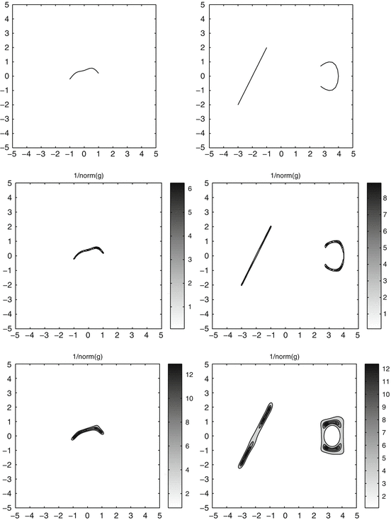
The true object (top), reconstruction with 0. 5 % noise (middle), and with 5 % noise (bottom). The wave number is k = 3
-
3.
The curve given by the parametric equation (Fig. 8.12, top left)
$$\displaystyle{\varGamma:= \left\{\varrho (s) = \left(s,0.5\cos \frac{\pi s} {2} + 0.2\sin \frac{\pi s} {2} - 0.1\cos \frac{3\pi s} {2} \right): -1 \leq s \leq 1\right\}.}$$ -
4.
Two disconnected curves described as in curves 1 and 2 above (Fig. 8.12, top right).


In all our examples, k = 3, and the far-field data are given for 32 incident directions and 32 observation directions equally distributed on the unit circle.
Notes
- 1.
Reprinted from F. Cakoni and D. Colton, The determination of the surface impedance of a partially coated obstacle from far-field data, SIAM J. Appl. Math. 64 (2004), 709–723. Copyright ©2004 Society for Industrial and Applied Mathematics. Reprinted with permission. All rights reserved.
- 2.
Reprinted from F. Cakoni, D. Colton, and P. Monk, The determination of the surface conductivity of a partially coated dielectric, SIAM J. Appl. Math. 65 (2005), 767–789. Copyright ©2005 Society for Industrial and Applied Mathematics. Reprinted with permission. All rights reserved.
- 3.
Reprinted from F. Cakoni and D. Colton, The linear sampling method for cracks, Inverse Problems 19 (2003), 279–295.
References
Aktosun T, Gintides D, Papanicolaou V (2011) The uniqueness in the inverse problem for transmission eigenvalues for the spherically symmetric variable-speed wave equation. Inverse Problems 27:115004.
Aktosun T, Papanicolaou V (2013) Reconstruction of the wave speed from transmission eigenvalues for the spherically symmetric variable-speed wave equation. Inverse Problems 29:065007.
Angell T, Kirsch A (1992) The conductive boundary condition for Maxwell’s equations. SIAM J. Appl. Math. 52:1597–1610.
Angell T, Kirsch A (2004) Optimization Methods in Electromagnetic Radiation. Springer, New York.
Arens T (2001) Linear sampling methods for 2D inverse elastic wave scattering. Inverse Problems 17:1445–1464.
Arens T (2004) Why linear sampling works. Inverse Problems 20:163–173.
Arens T, Lechleiter A(2009) The linear sampling method revisited. J. Integral Equations Appl. 21:179–203.
Boas Jr, Ralph P (1954) Entire Functions. Academic, New York.
Bonnet-BenDhia AS, Chesnel L, Haddar H (2011) On the use of t-coercivity to study the interior transmission eigenvalue problem. C. R. Acad. Sci., Ser. I 340:647–651.
Bonnet-BenDhia AS, Ciarlet P, Maria Zwölf C (2010) Time harmonic wave diffraction problems in materials with sign-shifting coefficients. J. Comput. Appl. Math 234:1912–1919.
Bressan A (2013) Lecture Notes on Functional Analysis with Applications to Linear Partial Differential Equations. American Mathematical Society, Providence, RI.
Buchanan JL, Gilbert RP, Wirgin A, Xu Y (2004) Marine Acoustics. Direct and Inverse Problems. SIAM, Philadelphia.
Cakoni F, Colton D (2003) A uniqueness theorem for an inverse electomagnetic scattering problem in inhomogeneous anisotropic media. Proc. Edinb. Math. Soc. 46:293–314.
Cakoni F, Colton D (2003) On the mathematical basis of the linear sampling method. Georgian Math. J. 10/3:411–425.
Cakoni F, Colton D (2003) The linear sampling method for cracks. Inverse Problems 19:279–295.
Cakoni F, Colton D (2003) Combined far field operators in electromagnetic inverse scattering theory. Math. Methods Appl. Sci. 26:413–429.
Cakoni F, Colton D (2004) The determination of the surface impedance of a partially coated obstacle from far field data. SIAM J. Appl. Math. 64:709–723.
Cakoni F, Colton D (2005) Open problems in the qualitative approach to inverse electromagnetic scattering theory. Eur. J. Appl. Math. to appear.
Cakoni F, Colton D, Gintides D (2010) The interior transmission eigenvalue problem. SIAM J. Math. Anal. 42:2912–2921.
Cakoni F, Colton D, Haddar H (2002) The linear sampling method for anisotropic media. J. Comp. Appl. Math. 146:285–299.
Cakoni F, Colton D, Haddar H (2009) The computation of lower bounds for the norm of the index of refraction in an anisotropic media. J. Integral Equations Appl. 21(2):203–227.
Cakoni F, Colton D, Haddar H (2010) On the determination of Dirichlet or transmission eigenvalues from far field data. C. R. Math. Acad. Sci. Paris, Ser I 348(7–8):379–383.
Cakoni F, Colton D, Monk P (2001) The direct and inverse scattering problems for partially coated obstacles. Inverse Problems 17:1997–2015.
Cakoni F, Colton D, Monk P (2004) The electromagnetic inverse scattering problem for partly coated Lipschitz domains. Proc. R. Soc. Edinb. 134A:661–682.
Cakoni F, Colton D, Monk P (2010) The determination of boundary coefficients from far field measurements. J. Int. Equations Appl. 42(2):167–191.
Cakoni F, Colton D, Monk P (2011) The Linear Sampling Method in Inverse Electromagnetic Scattering. CBMS-NSF Regional Conference Series in Applied Mathematics 80, SIAM, Philadelphia.
Cakoni F, Colton D, Monk P (2005) The determination of the surface conductivity of a partially coated dielectric. SIAM J. Appl. Math. 65:767–789.
Cakoni F, Colton D, Monk P, Sun J (2010) The inverse electromagnetic scattering problem for anisotropic media. Inverse Problems 26:074004.
Cakoni F, Darrigrand E (2005) The inverse electromagnetic scattering problem for a mixed boundary value problem for screens. J. Comp. Appl. Math. 174:251–269.
Cakoni F, Fares M, Haddar H (2006) Anals of two linear sampling methods applied to electromagnetic imaging of buried objects. Inverse Problems 42:237–255.
Cakoni F, Gintides D, Haddar H (2010) The existence of an infinite discrete set of transmission eigenvalues. SIAM J. Math. Anal. 42:237–255.
Cakoni F, Haddar H (2013) Transmission eigenvalues in inverse scattering theory Inverse Problems and Applications, Inside Out 60, MSRI Publications, Berkeley, CA.
Cakoni F, Haddar H (2008), On the existence of transmission eigenvalues in an inhomogeneous medium. Applicable Anal. 88(4):475–493.
Cakoni F, Haddar H (2003) Interior transmission problem for anisotropic media. Mathematical and Numerical Aspects of Wave Propagation (Cohen et al., eds.), Springer, 613–618.
Cakoni F, Kirsch A (2010) On the interior transmission eigenvalue problem (2010) Int. J. Comp. Sci. Math. 3:142–167.
Chanillo S, Helffer B, Laptev A (2004) Nonlinear eigenvalues and analytic hypoellipticity. J. Functional Analysis 209:425–443.
Charalambopoulos A, Gintides D, Kiriaki K (2002) The linear sampling method for the transmission problem in three-dimensional linear elasticity. Inverse Problems 18:547–558.
Charalambopoulos A, Gintides D, Kiriaki K (2003) The linear sampling method for non-absorbing penetrable elastic bodies. Inverse Problems 19:549–561.
Chesnel L (2012) Étude de quelques problémes de transmission avec changement de signe. Application aux métamatériaux. Ph.D. thesis. École Doctorale de l’École Polytechnique, France.
Chesnel L (2012) Interior transmission eigenvalue problem for Maxwell’s equations: the T-coercivity as an alternative approach. Inverse Problems 28:065005.
Cheng J, Yamamoto M (2003) Uniqueness in an inverse scattering problem within non-trapping polygonal obstacles with at most two incoming waves. Inverse Problems 19:1361–1384.
Collino F, Fares M, Haddar H (2003) Numerical and analytical studies of the linear sampling method in electromagnetic inverse scattering problems. Inverse Problems 19:1279–1298.
Colton D (2004) Partial Differential Equations: An Introduction. Dover, New York.
Colton D, Coyle J, Monk P (2000) Recent developments in inverse acoustic scattering theory. SIAM Rev. 42:369–414.
Colton D (1980) Analytic Theory of Partial Differential Equations. Pitman Advanced Publishing Program, Boston.
Colton D, Erbe C (1996) Spectral theory of the magnetic far field operator in an orthotropic medium, in Nonlinear Problems in Applied Mathematics, SIAM, Philadelphia.
Colton D, Haddar H (2005) An application of the reciprocity gap functional to inverse scattering theory. Inverse Problems 21:383–398.
Colton D, Haddar H, Monk P (2002) The linear sampling method for solving the electromagnetic inverse scattering problem. SIAM J. Sci. Comput. 24:719–731.
Colton D, Haddar H, Piana P (2003) The linear sampling method in inverse electromagnetic scattering theory. Inverse Problems 19:S105–S137.
Colton D, Kirsch A (1996) A simple method for solving inverse scattering problems in the resonance region. Inverse Problems 12:383–393.
Colton D, Kress R (1983) Integral Equation Methods in Scattering Theory. Wiley, New York.
Colton D, Kress R (1995) Eigenvalues of the far field operator and inverse scattering theory. SIAM J. Math. Anal. 26:601–615.
Colton D, Kress R (1995) Eigenvalues of the far field operator for the Helmholtz equation in an absorbing medium. SIAM J. Appl. Math. 55:1724–35.
Colton D, Kress R (2013) Inverse Acoustic and Electromagnetic Scattering Theory, 3rd edn. Springer, New York.
Colton D, Kress R (2001) On the denseness of Herglotz wave functions and electromagnetic Herglotz pairs in Sobolev spaces. Math. Methods Appl. Sci. 24:1289–1303.
Colton D, Leung YJ (2013) Complex eigenvalues and the inverse spectral problem for transmission eigenvalues. Inverse Problems. 29:104008.
Colton D, Kress R, Monk P. (1997) Inverse scattering from an orthotropic medium. J. Comp. Appl. Math. 81:269–298.
Colton D, Monk P. (1999) A linear sampling method for the detection of leukemia using microwaves. II. SIAM J. Appl. Math. 69, 241–255.
Colton D, Päivarinta L (1992) The uniqueness of a solution to an inverse scattering problem for electromagnetic wave. Arch. Rational Mech. Anal. 119:59–70.
Colton D, Päivärinta L, Sylvester J (2007) The interior transmission problem. Inverse Problems Imag. 1:13–28.
Colton D, Piana M, Potthast R (1997) A simple method using Morozov’s discrepancy principle for solving inverse scattering problems. Inverse Problems 13:1477–1493.
Colton D, Sleeman BD (1983) Uniqueness theorems for the inverse problem of acoustic scattering. IMA J. Appl. Math. 31:253–59.
Colton D, Sleeman BD (2001) An approximation property of importance in inverse scattering theory. Proc. Edinb. Math. Soc. 44:449–454.
Costabel M, Dauge M (2002) Crack singularities for general elliptic systems. Math. Nachr. 235:29–49.
Costabel M, Dauge M (1996) A singularly perturbed mixed boundary value problem. Comm. Partial Differential Equations 21:1919–1949.
Cossonnière A, Haddar H (2011) The electromagnetic interior transmission problem for regions with cavities. SIAM J. Math. Anal. 43:1698–1715.
Coyle J (2000) An inverse electromagnetic scattering problem in a two-layered background. Inverse Problems 16:275–292.
Engl HW, Hanke M, Neubauer A (1996) Regularization of Inverse Problems. Kluwer, Dordrecht.
Fredholm I (1903) Sur une classe d’équations fonctionelles. Acta Math. 27:365–390.
Friedman A (1969) Partial Differential Equations. Holt, Rinehart and Winston, New York.
Ghosh Roy DN, Couchman LS (2002) Inverse Problems and Inverse Scattering of Plane Waves. Academic, London.
Gilbarg D, Trudinger NS (1983) Elliptic Partial Differential Equations of Second Order, 2nd edn. Springer, Berlin.
Gintides D, Kiriaki K (2001) The far-field equations in linear elasticity – an inversion scheme. Z. Angew. Math. Mech. 81:305–316.
Griesmaier R, Hanke M, Sylvester J (to appear) Far field splitting for the Helmholtz equation.
Grinberg NI, Kirsch A (2002) The linear sampling method in inverse obstacle scattering for impedance boundary conditions. J. Inv. Ill-Posed Problems 10:171–185.
Grinberg NI, Kirsch A (2004) The factorization method for obstacles with a-priori separated sound-soft and sound-hard parts. Math. Comput. Simulation 66:267–279
Gylys-Colwell F (1996) An inverse problem for the Helmholtz equation. Inverse Problems 12:139–156.
Haddar H (2004) The interior transmission problem for anisotropic Maxwell’s equations and its applications to the inverse problem. Math. Methods Appl. Sci. 27:2111–2129.
Haddar H, Joly P (2002)Stability of thin layer approximation of electromagnetic waves scattering by linear and nonlinear coatings. J. Comp. Appl. Math. 143:201–236.
Haddar H, Monk P (2002) The linear sampling method for solving the electromagnetic inverse medium problem. Inverse Problems 18:891–906.
Hähner P (2000) On the uniqueness of the shape of a penetrable, anisotropic obstacle. J. Comp. Appl. Math. 116:167–180.
Hähner P (2002) Electromagnetic wave scattering: theory. in Scattering (Pike and Sabatier, eds.) Academic, New York.
Hartman P, Wilcox C (1961) On solutions of the Helmholtz equation in exterior domains. Math. Zeit. 75:228–255.
Hitrik M, Krupchyk K, Ola P, Päivärinta L (2010) Transmission eigenvalues for operators with constant coefficients. SIAM J. Math. Anal. 42:2965–2986.
Hitrik M, Krupchyk K, Ola P and Päivärinta L (2011) The interior transmission problem and bounds on transmission eigenvalues. Math Res. Lett. 18:279–293.
Hitrik M, Krupchyk K, Ola P, Päivärinta L (2011) Transmission eigenvalues for elliptic operators. SIAM J. Math. Anal. 43:2630–2639.
Hochstadt H (1973) Integral Equations. Wiley, New York.
Hooper AE, Hambric HN (1999) Unexploded ordinance (UXO): The problem. Detection and Identification of Visually Obscured Targets (Baum, ed.), Taylor and Francis, Philadelphia.
Hörmander L (1985) The Analysis of Linear Partial Differential Operators III. Springer, Berlin.
Hsiao G, Wendland WL (2008) Boundary Integral Equations. Springer, Berlin.
Ikehata M (1998) Reconstruction of the shape of an obstacle from scattering amplitude at a fixed frequency. Inverse Problems 14:949–954.
Ikehata M (1999) Reconstructions of obstacle from boundary measurements. Waves Motion 30:205–223.
Isakov V (1988) On the uniqueness in the inverse transmission scattering problem. Comm. Partial Differential Equations 15:1565–1587.
Isakov V (1998) Inverse Problems for Partial Differential Equations. Springer, New York.
John F (1982) Partial Differential Equations, 4th ed. Springer Verlag, New York.
Jones DS (1974) Integral equations for the exterior acoustic problem. Q. J. Mech. Appl. Math. 27:129–142.
Y. Katznelson (9168) An Introduction to Harmonic Analysis. Wiley, New York.
Kirsch A (2011) An Introduction to the Mathematical Theory of Inverse Problems, 2nd edn. Springer, New York.
Kirsch A (1998) Characterization of the shape of a scattering obstacle using the spectral data of the far field operator. Inverse Problems 14:1489–1512.
Kirsch A (1999) Factorization of the far field operator for the inhomogeneous medium case and an application in inverse scattering theory. Inverse Problems 15:413–29.
Kirsch A (2002) The MUSIC-algorithm and the factorization method in inverse scattering theory for inhomogeneous media. Inverse Problems 18:1025–1040.
Kirsch A (2004) The factorization method for Maxwell’s equations. Inverse Problems 20:S117-S134.
Kirsch A (2005) The factorization method for a class of inverse elliptic problems. Math. Nachr. 278:258–277.
Kirsch A (2008) An integral equation for the scattering problem for an anisotropic medium and the factorization method. Advanced Topics in Scattering and Biomedical Engineering, Proceedings of the 8th International Workshop on Mathematical Methods in Scattering Theory and Biomedical Engineering. World Scientific, New Jersey.
Kirsch A (2009) On the existence of transmission eigenvalues. Inverse Problems Imag. 3:155–172.
Kirsch A, Kress R (1993) Uniqueness in inverse obstacle scattering. Inverse Problems 9:81–96.
Kirsch A, Grinberg N (2008) The Factorization Method for Inverse Problems. Oxford University Press, Oxford.
Kirsch A, Ritter S (2000) A linear sampling method for inverse scattering from an open arc. Inverse Problems 16:89–105.
Kleinman RE, Roach GF (1982) On modified Green’s functions in exterior problems for the Helmholtz equation. Proc. R. Soc. Lond. A383:313–332.
Kress R (1995) Inverse scattering from an open arc. Math. Methods Appl. Sci. 18:267–293.
Kress R (1999) Linear Integral Equations, 2nd edn. Springer, New York.
Kress R, Lee KM (2003) Integral equation methods for scattering from an impedance crack. J. Comp. Appl. Math. 161:161–177.
Kress R, Rundell W (2001) Inverse scattering for shape and impedance. Inverse Problems 17:1075–1085.
Kress R, Serranho P (2005) A hybrid method for two-dimensional crack reconstruction. Inverse Problems 21:773–784.
Kreyszig E (1978) Introductory Functional Analysis with Applications. Wiley, New York.
Kusiak S, Sylvester J (2003) The scattering support. Comm. Pure Appl. Math. 56:1525–1548.
Kusiak S, Sylvester J (2005) The convex scattering support in a background medium. SIAM J. Math. Anal. 36:1142–1158.
Lakshtanov E, Vainberg B (2012) Bounds on positive interior transmission eigenvalues. Inverse Problems 28:105005.
Lakshtanov E, Vainberg B (2012) Remarks on interior transmission eigenvalues, Weyl formula and branching billiards. J. Phys. A 25 12:125202.
Lakshtanov E, Vainberg B (2012) Ellipticity in the interior transmission problem in anisotropic media. SIAM J. Math. Anal. 44 2:1165–1174.
Lebedev NN (1965) Special Functions and Their Applications. Prentice-Hall, Englewood Cliffs, NJ.
Leung YJ, Colton D (2012) Complex transmission eigenvalues for spherically stratified media. Inverse Problems 28:2944956.
Levin B Y (1996) Lectures on Entire Functions. American Mathematical Society. Providence, RI.
Lions J, Magenes E (1972) Non-homogeneous Boundary Value Problems and Applications. Springer, New York.
Magnus W (1949) Fragen der Eindeutigkeit und des Verhattens im Unendlichen für Lösungen von Δ u + k 2 u = 0. Abh. Math. Sem. Hamburg 16:77–94.
McLaughlin JR, Polyakov PL (1994) On the uniqueness of a spherically symmetric speed of sound from transmission eigenvalues. J. Differential Equations 107:351–382.
McLean W (2000) Strongly Elliptic Systems and Boundary Integral Equations. Cambridge University Press, Cambridge.
Mönch L (1997) On the inverse acoustic scattering problem by an open arc: the sound-hard case. Inverse Problems 13:1379–1392
Monk P (2003) Finite Element Methods for Maxwell’s Equations. Oxford University Press, Oxford.
Morozov VA (1984) Methods for Solving Incorrectly Posed Problems. Springer, New York.
Müller C (1952) Über die ganzen Lösungen der Wellengleichung. Math. Annalen 124:235–264
Nintcheu Fata S, Guzina BB (2004) A linear sampling method for near-field inverse problems in elastodynamics. Inverse Problems 20:713–736.
Norris AN (1998) A direct inverse scattering method for imaging obstacles with unknown surface conditions. IMA J. Applied Math. 61:267–290.
Päivärinta L, Sylvester J. (2008) Transmission eigenvalues. SIAM J. Math. Anal. 40 738–753.
Pelekanos G, Sevroglou V (2003) Inverse scattering by penetrable objects in two-dimensional elastodynamics. J. Comp. Appl. Math. 151:129–140.
Piana M (1998) On uniqueness for anisotropic inhomogeneous inverse scattering problems. Inverse Problems 14:1565–1579.
Potthast R (1999) Electromagnetic scattering from an orthotropic medium. J. Integral Equations Appl. 11:197–215.
Potthast R (2000) Stability estimates and reconstructions in inverse acoustic scattering using singular sources. J. Comp. Appl. Math. 114:247–274.
Potthast R (2001) Point Sourse and Multipoles in Inverse Scattering Theory. Research Notes in Mathematics, Vol 427, Chapman and Hall/CRC, Boca Raton, FL.
Potthast R (2004) A new non-iterative singular sources method for the reconstruction of piecewise constant media. Numer. Math. 98:703–730.
Potthast R, Sylvester J, Kusiak S (2003) A ’range test’ for determining scatterers with unknown physical properties. Inverse Problems 19:533–47.
Pöschel J, Trubowitz E (1987) Inverse Spectral Theory. Academic, Boston.
Rellich F (1943) Über das asymptotische Verhalten der Lösungen von △ u +λ u = 0 im unendlichen Gebieten. Jber. Deutsch. Math. Verein. 53:57–65.
Riesz F (1918) Über lineare Funktionalgleichungen. Acta Math. 41:71–98.
Robert D (2004) Non-linear eigenvalue problems. Mat. Contemp. 26:109–127.
Rondi L (2003) Unique determination of non-smooth sound-soft scatteres by finitely many far field measurements. Indiana University Math. J. 52:1631–62.
Rundell W, Sacks P (1992) Reconstruction techniques for classical inverse Sturm-Liouville problems. Math. Comput. 58:161–183.
Rynne BP, Sleeman BD (1991) The interior transmission problem and inverse scattering from inhomogeneous media. SIAM J. Math. Anal. 22:1755–1762.
Schechter M (2002) Principles of Functional Analysis, 2nd edn. American Mathematical Society, Providence, RI.
Sevroglou V (2005) The far-field operator for penetrable and absorbing obstacles in 2D inverse elastic scattering. Inverse Problems 21:717–738.
Stefanov P, Uhlmann G (2004) Local uniqueness for the fixed energy fixed angle inverse problem in obstacle scattering. Proc. Am. Math. Soc. 132:1351–54.
Stephan EP (1987) Boundary integral equations for screen problems in ℝ 3. Integral Equations Operator Theory 10:236–257.
Stephan EP, Wendland W (1984) An augmented Galerkin procedure for the boundary integral method applied to two-dimensional screen and crack problems. Appl. Anal. 18:183–219.
Sylvester J (2012) Discreteness of transmission eigenvalues via upper triangular compact operator. SIAM J. Math. Anal. 44:341–354.
Tacchino A, Coyle J, Piana M (2002) Numerical validation of the linear sampling method. Inverse Problems 18:511–527.
Ursell F (1978) On the exterior problems of acoustics II. Proc. Cambridge Phil. Soc. 84:545–548.
Vekua IN (1943) Metaharmonic functions. Trudy Tbilisskogo Matematichesgo Instituta 12:105–174.
Xu Y, Mawata C, Lin W (2000) Generalized dual space indicator method for underwater imaging. Inverse Problems 16:1761–1776.
You YX, Miao GP (2002) An indicator sampling method for solving the inverse acoustic scattering problem from penetrable obstacles. Inverse Problems 18:859–880.
You YX, Miao GP, Liu YZ (2000) A fast method for acoustic imaging of multiple three-dimensional objects. J. Acoust. Soc. Am. 108:31–37.
Young RM (2001) An Introduction to Nonharmonic Fourier Series. Academic, San Diego.
Author information
Authors and Affiliations
Rights and permissions
Copyright information
© 2014 Springer Science+Business Media New York
About this chapter
Cite this chapter
Cakoni, F., Colton, D. (2014). Mixed Boundary Value Problems. In: A Qualitative Approach to Inverse Scattering Theory. Applied Mathematical Sciences, vol 188. Springer, Boston, MA. https://doi.org/10.1007/978-1-4614-8827-9_8
Download citation
DOI: https://doi.org/10.1007/978-1-4614-8827-9_8
Published:
Publisher Name: Springer, Boston, MA
Print ISBN: 978-1-4614-8826-2
Online ISBN: 978-1-4614-8827-9
eBook Packages: Mathematics and StatisticsMathematics and Statistics (R0)