Verification of Sequential Programs

Abstract

A computer program is not very different from a logical formula. It consists of a sequence of symbols constructed according to formal syntactical rules and it has a meaning which is assigned by an interpretation of the elements of the language. In programming, the symbols are called statements or commands and the intended interpretation is the execution of the program on a computer. The syntax of programming languages is specified using formal systems such as BNF, but the semantics is usually informally specified.

These keywords were added by machine and not by the authors. This process is experimental and the keywords may be updated as the learning algorithm improves.

A computer program is not very different from a logical formula. It consists of a sequence of symbols constructed according to formal syntactical rules and it has a meaning which is assigned by an interpretation of the elements of the language. In programming, the symbols are called statements or commands and the intended interpretation is the execution of the program on a computer. The syntax of programming languages is specified using formal systems such as BNF, but the semantics is usually informally specified.

In this chapter, we describe a formal semantics for a simple programming language, as well as a deductive system for proving that a program is correct. Unlike our usual approach, we first define the deductive system and only later define the formal semantics. The reason is that the deductive system is useful for proving programs, but the formal semantics is primarily intended for proving the soundness and completeness of the deductive system.

The chapter is concerned with sequential programs. A different, more complex, logical formalism is needed to verify concurrent programs and this is discussed separately in Chap. 16.

Our programs will be expressed using a fragment of the syntax of popular languages like Java and C. A program is a statement S, where statements are defined recursively using the concepts of variables and expressions:

We assume that the informal semantics of programs written in this syntax is familiar. In particular, the concept of the location counter (sometimes called the instruction pointer) is fundamental: During the execution of a program, the location counter stores the address of the next instruction to be executed by the processor.

In our examples the values of the variables will be integers.

15.1 Correctness Formulas

A statement in a programming language can be considered to be a function that transforms the state of a computation. If the variables (x,y) have the values (8,7) in a state, then the result of executing the statement x = 2*y+1 is the state in which (x,y)=(15,7) and the location counter is incremented.

Definition 15.1

Let S be a program with n variables (x1,…,xn). A state s of S consists of an n+1-tuple of values (lc,x ₁,…,x _n ), where lc is the value of the location counter and x _i is the value of the variable xi. ■

The variables of a program will be written in typewriter font x, while the corresponding value of the variable will be written in italic font x. Since a state is always associated with a specific location, the location counter will be implicit and the state will be an n-tuple of the values of the variables.

In order to reason about programs within first-order logic, predicates are used to specify sets of states.

Definition 15.2

Let U be the set of all n-tuples of values over some domain(s), and let U′⊆U be a relation over U. The n-ary predicate P _U′ is the characteristic predicate of U′ if it is interpreted over the domain U by the relation U′. That is, v(P _U′(x ₁,…,x _n ))=T iff (x ₁,…,x _n )∈U′. ■

We can write {(x ₁,…,x _n )∣(x ₁,…,x _n )∈U′} as {(x ₁,…,x _n )∣P _U′}.

Example 15.3

Let U be the set of 2-tuples over $Z$ and let U′⊆U be the 2-tuples described in the following table:

$$ \begin{array}{*{20}r} {} & {} & {} & {} & \ldots & {} & {} & {} \\ \ldots & {( - 2, - 3)} & {( - 2, - 2)} & {( - 2, - 1)} & {( - 2,0)} & {( - 2,1)} & {( - 2,2)} & {( - 2,3)} \\ \ldots & {( - 1, - 3)} & {( - 1, - 2)} & {( - 1, - 1)} & {( - 1,0)} & {( - 1,1)} & {( - 1,2)} & {( - 1,3)} \\ \ldots & {(0, - 3)} & {(0, - 2)} & {(0, - 1)} & {(0,0)} & {(0,1)} & {(0,2)} & {(0,3)} \\ \ldots & {(1, - 3)} & {(1, - 2)} & {(1, - 1)} & {(1,0)} & {(1,1)} & {(1,2)} & {(1,3)} \\ \ldots & {(2, - 3)} & {(2, - 2)} & {(2, - 1)} & {(2,0)} & {(2,1)} & {(2,2)} & {(2,3)} \\ \end{array} $$

Two characteristic predicates of U′ are (x ₁=x ₁)∧(x ₂≤3) and x ₂≤3. The set can be written as {(x ₁,x ₂)∣x ₂≤3}. ■

The semantics of a programming language is given by specifying how each statement in the language transforms one state into another.

Example 15.4

Let S be the statement x = 2*y+1. If started in an arbitrary state (x,y), the statement terminates in the state (x′,y′) where x′=2y′+1. Another way of expressing this is to say that S transforms the set of states {(x,y)∣true} into the set {(x,y)∣x=2y+1}.

The statement S also transforms the set of states {(x,y)∣y≤3} into the set {(x,y)∣(x≤7)∧(y≤3)}, because if y≤3 then 2y+1≤7. ■

The concept of transforming a set of states can be extended from an assignment statement to the statement representing the entire program. This is then used to define correctness.

Definition 15.5

A correctness formula is a triple $\{p\}\:{\textup {\texttt {S}}}\:\{q\}$, where S is a program, and p and q are formulas called the precondition and postcondition, respectively. S is partially correct with respect to p and q, $\models \{p\}\:{\textup {\texttt {S}}}\:\{q\}$, iff:

If S is started in a state where p is true and if the computation of S terminates, then it terminates in a state where q is true. ■

Correctness formulas were first defined in Hoare (1969). The term is taken from Apt et al. (2009); the formulas are also called inductive expressions, inductive assertions and Hoare triples.

Example 15.6

$\models \{y\leq 3\}\:{\textup {\texttt {x = 2*y+1}}}\:\{(x\leq 7) \wedge (y \leq 3)\}$. ■

Example 15.7

For any S, p and q:

$$ \models \{\mathit{false}\}\:{\textup {\texttt {S}}}\:\{q\}, \qquad \models \{p\}\:{\textup {\texttt {S}}}\:\{\mathit{true}\}, $$

since false is not true in any state and true is true in all states. ■

15.2 Deductive System $HL$

The deductive system $HL$ (Hoare Logic) is sound and relatively complete for proving partial correctness. By relatively complete, we mean that the formulas expressing properties of the domain will not be formally proven. Instead, we will simply take all true formulas in the domain as axioms. For example, (x≥y)→(x+1≥y+1) is true in arithmetic and will be used as an axiom. This is reasonable since we wish to concentrate on the verification that a program S is correct without the complication of verifying arithmetic formulas that are well known.

Definition 15.8

(Deductive system $HL$)

Domain axioms :

$$\textrm{Every true formula over the domain(s) of the program variables.}$$

Assignment axiom :

$$\vdash \{p(x)\{x\leftarrow t\}\}\:{\textup {\texttt {x\ =\ t}}}\:\{p(x)\}. $$

Composition rule :

$$\frac{\vdash \{p\}\:{\textup {\texttt {S1}}}\:\{q\}\hspace{4em}\vdash \{q\}\:{\textup {\texttt {S2}}}\:\{r\}}{\vdash \{p\}\:{\textup {\texttt {S1 S2}}}\:\{r\}}.$$

Alternative rule :

$$\frac{\vdash \{p\wedge B\}\:{\textup {\texttt {S1}}}\:\{q\}\hspace{4em} \vdash \{p\wedge \neg \,B\}\:{\textup {\texttt {S2}}}\:\{q\}}{\vdash \{p\}\:{\textup {\texttt {if\ (B)\ S1\ else\ S2}}}\:\{q\}}.$$

Loop rule :

$$\frac{\vdash \{p\wedge B\}\:{\textup {\texttt {S}}}\:\{p\}}{\vdash \{p\}\:{\textup {\texttt {while\ (B)\ S}}}\:\{p\wedge \neg \,B\}}.$$

Consequence rule :

$$\frac{\vdash p_{1}\mathbin {\rightarrow }p\hspace{3em}\vdash \{p\}\:{\textup {\texttt {S}}}\:\{q\}\hspace{3em}\vdash q\mathbin {\rightarrow }q_{1}}{\vdash \{p_{1}\}\:{\textup {\texttt {S}}}\:\{q_{1}\}}.$$

 ■

The consequence rule says that we can always strengthen the precondition or weaken the postcondition.

Example 15.9

From Example 15.6, we know that:

$$ \models \{y\leq 3\}\:{\textup {\texttt {x = 2*y+1}}}\:\{(x\leq 7) \wedge (y \leq 3)\}. $$

Clearly:

$$ \models \{y\leq 1\}\:{\textup {\texttt {x = 2*y+1}}}\:\{(x\leq 10) \wedge (y \leq 3)\}. $$

The states satisfying y≤1 are a subset of those satisfying y≤3, so a computation started in a state where, say, y=0≤1 satisfies y≤3. Similarly, the states satisfying x≤10 are a superset of those satisfying x≤7; we know that the computation results in a value of x such that x≤7 and that value is also less than or equal to 10. ■

Since ⊢p→p and ⊢q→q, we can strengthen the precondition without weakening the postcondition or conversely.

The assignment axiom may seem strange at first, but it can be understood by reasoning from the conclusion to the premise. Consider:

$$\vdash \{?\}\:{\textup {\texttt {x\ =\ t}}}\:\{p(x)\}.$$

After executing the assignment statement, we want p(x) to be true when the value assigned to x is the value of the expression t. If the formula that results from performing the substitution p(x){x←t} is true, then when x is actually assigned the value of t, p(x) will be true.

The composition rule and the alternative rule are straightforward.

The formula p in the loop rule is called an invariant: it describes the behavior of a single execution of the statement S in the body of the while-statement. To prove:

$$\vdash \{p_{0}\}\:{\textup {\texttt {while\ (B)\ S}}}\:\{q_0\},$$

we find a formula p and prove that it is an invariant: $\vdash \{p\wedge B\}\:{\textup {\texttt {S}}}\:\{p\}$.

By the loop rule:

$$\vdash \{p\}\:{\textup {\texttt {while\ (B)\ S}}}\:\{p\wedge \neg \,B\}.$$

If we can prove p ₀→p and (p∧¬ B)→q ₀, then the consequence rule can be used to deduce the correctness formula. We do not know how many times the while-loop will be executed, but we know that p∧¬ B holds when it does terminate.

To prove the correctness of a program, one has to find appropriate invariants. The weakest possible formula true is an invariant of any loop since $\vdash \{\mathit{true}\wedge B\}\:{\textup {\texttt {S}}}\:\{\mathit{true}\}$ holds for any B and S. Of course, this formula is too weak, because it is unlikely that we will be able to prove (true∧¬ B)→q ₀. On the other hand, if the formula is too strong, it will not be an invariant.

Example 15.10

x=5 is too strong to be an invariant of the while-statement:

because x=5∧x>0 clearly does not imply that x=5 after executing the statement x = x - 1. The weaker formula x≥0 is also an invariant: x≥0∧x>0 implies x≥0 after executing the loop body. By the loop rule, if the loop terminates then x≥0∧¬ (x>0). This can be simplified to x=0 by reasoning within the domain and using the consequence rule. ■

15.3 Program Verification

Let us use $HL$ to proving the partial correctness of the following program P:

Be careful to distinguish between braces { } used in the syntax of the program from those used in the correctness formulas.

We have annotated P with formulas between the statements. Given:

$$\{p_{1}\}\textup {\texttt {S1}}\{p_{2}\}\textup {\texttt {S2}}\cdots\{p_{n}\}\textup {\texttt {Sn}}\{p_{n+1}\},$$

if we can prove $\{p_{i}\}\:{\textup {\texttt {Si}}}\:\{p_{i+1}\}$ for all i, then we can conclude:

$$\{p_{1}\}\:{\textup {\texttt {S1 $\cdots$ Sn}}}\:\{p_{n+1}\}$$

by repeated application of the composition rule. See Apt et al. (2009, Sect. 3.4) for a proof that $HL$ with annotations is equivalent to $HL$ without them.

Theorem 15.11

$\vdash \{\mathit{true}\}\:{\textup {\texttt {P}}}\:\{x=a\cdot b\}$.

Proof

From the assignment axiom we have $\{0=0\}\:{\textup {\texttt {x=0}}}\:\{x=0\}$, and from the consequence rule with premise true→(0=0), we have $\{\mathit{true}\}\:{\textup {\texttt {x=0}}}\:\{x=0\}$. The proof of $\{x=0\}\:{\textup {\texttt {y=b}}}\:\{(x=0) \wedge (y=b)\}$ is similar.

Let us now show that x=(b−y)⋅a is an invariant of the loop. Executing the loop body will substitute x+a for x and y−1 for y. Since the assignments have no variable in common, we can do them simultaneously. Therefore:

$$ \begin{array}{r@{\ \ \ }l@{\ \ \ }l} (x=(b-y)\cdot a )\{x\leftarrow x+a, y \leftarrow y-1\} &\mathrel {\equiv }& x+a=(b-(y-1))\cdot a\\[2pt] &\mathrel {\equiv }& x=(b-y+1)\cdot a - a\\[2pt] &\mathrel {\equiv }& x=(b-y)\cdot a +a - a\\[2pt] &\mathrel {\equiv }& x=(b-y)\cdot a. \end{array} $$

By the consequence rule, we can strengthen the precondition:

$$\{(x=(b-y)\cdot a)\wedge y\neq 0\}\:{\textup {\texttt {x=x+a;\ y=y-1;}}}\:\{x=(b-y)\cdot a\},$$

and then use the Loop Rule to deduce:

Since ¬ (y≠0)≡(y=0), we obtain the required postcondition:

$$ (x=(b-y)\cdot a) \wedge (y = 0) \mathrel {\equiv }(x=b\cdot a) \mathrel {\equiv }(x=a\cdot b). $$

 ■

15.3.1 Total Correctness *

Definition 15.12

A program S is totally correct with respect to p and q iff:

If S is started in a state where p is true, then the computation of S terminates and it terminates in a state where q is true. ■

The program in Sect. 15.3 is partial correct but not totally correct: if the initial value of b is negative, the program will not terminate. The precondition needs to be strengthened to b≥0 for the program to be totally correct.

Clearly, the only construct in a program that can lead to non-termination is a loop statement, because the number of iterations of a while-statement need not be bounded. Total correctness is proved by showing that the body of the loop always decreases some value and that that value is bounded from below. In the above program, the value of the variable y decreases by one during each execution of the loop body. Furthermore, it is easy to see that y≥0 can be added to the invariant of the loop and that y is bounded from below by 0. Therefore, if the precondition is b≥0, then b≥0→y≥0 and the program terminates when y=0.

$HL$ can be extended to a deductive system for total correctness; see Apt et al. (2009, Sect. 3.3).

15.4 Program Synthesis

Correctness formulas may also be used in the synthesis of programs: the construction of a program directly from a formal specification. The emphasis is on finding invariants of loops, because the other aspects of proving a program (aside from deductions within the domain) are purely mechanical. Invariants are hypothesized as modifications of the postcondition and the program is constructed to maintain the truth of the invariant. We demonstrate the method by developing two different programs for finding the integer square root of a non-negative integer $x=\lfloor \sqrt{a} \rfloor$; expressed as a correctness formula using integers, this is:

$$\{0\leq a\}\:{\textup {\texttt {S}}}\:\{0\leq x^{2} \leq a < (x+1)^{2}\}.$$

15.4.1 Solution 1

A loop is used to calculate values of the variable x until the postcondition holds. Suppose we let the first part of the postcondition be the invariant and try to establish the second part upon termination of the loop. This gives the following program outline, where E1(x,a), E2(x,a) and B(x,a) represent expressions that must be determined:

Let p denote the formula 0≤x ²≤a that is the first subformula of the postcondition and then see what expressions will make p an invariant:

• The precondition is 0≤a, so p will be true at the beginning of the loop if the first statement is x=0.

• By the loop rule, when the while-statement terminates, the formula p∧¬ B(x,a) is true. If this formula implies the postcondition:

  $$ (0\leq x^{2}\leq a) \wedge \neg \,B(x,a) \mathbin {\rightarrow }0\leq x^{2}\leq a < (x+1)^{2}, $$

  the postcondition follows by the consequence rule. Clearly, ¬ B(x,a) should be a<(x+1)², so we choose B(x,a) to be (x+1)*(x+1)<=a.

• Given this Boolean expression, if the loop body always increases the value of x, then the loop will terminate. The simplest way to do this is x=x+1.

Here is the resulting program:

What remains to do is to check that p is, in fact, an invariant of the loop: $\{p\wedge B\}\:{\textup {\texttt {S}}}\:\{p\}$. Written out in full, this is:

$$\{0\leq x^{2}\leq a \wedge (x+1)^{2}\leq a\}\:{\textup {\texttt {x=x+1}}}\:\{0\leq x^{2}\leq a\}.$$

The assignment axiom for x=x+1 is:

$$\{0\leq (x+1)^{2}\leq a\}\:{\textup {\texttt {x=x+1}}}\:\{0\leq x^{2}\leq a\}.$$

The invariant follows from the consequence rule if the formula:

$$(0\leq x^{2}\leq a \wedge (x+1)^{2}\leq a) \mathbin {\rightarrow }(0\leq (x+1)^{2}\leq a)$$

is provable. But this is a true formula of arithmetic so it is a domain axiom.

15.4.2 Solution 2

Incrementing the variable x is not a very efficient way of computing the integer square root. With some more work, we can find a better solution. Let us introduce a new variable y to bound x from above; if we maintain x<y while increasing the value of x or decreasing the value of y, we should be able to close in on a value that makes the postcondition true. Our invariant will contain the formula:

$$0\leq x^{2}\leq a < y^{2}.$$

Looking at the postcondition, we see that y is overestimated by a+1, so a candidate for the invariant p is:

$$(0\leq x^{2}\leq a < y^{2})\wedge (x < y\leq a+1).$$

Before trying to establish p as an invariant, let us check that we can find an initialization statement and a Boolean expression that will make p true initially and the postcondition true when the loop terminates.

• The statement y=a+1 makes p true at the beginning of the loop.

• If the loop terminates when ¬ B is y=x+1, then:

  $$ p \wedge \neg \,B \mathbin {\rightarrow }0\leq x^{2}\leq a < (x+1)^{2}. $$

The outline of the program is:

Before continuing with the synthesis, let us try an example.

Example 15.13

Suppose that a=14. Initially, x=0 and y=15. The loop should terminate when x=3 and y=x+1=4 so that 0≤9≤14<16. We need to increase x or decrease y while maintaining the invariant 0≤x ²≤a<y ². Let us take the midpoint ⌊(x+y)/2⌋=⌊(0+15)/2⌋=7 and assign it to either x or y, as appropriate, to narrow the range. In this case, a=14<49=7⋅7, so assigning 7 to y will maintain the invariant. On the next iteration, ⌊(x+y)/2⌋=⌊(0+7)/2⌋=3 and 3⋅3=9<14=a, so assigning 3 to x will maintain the invariant. After two more iterations during which y receives the values 5 and then 4, the loop terminates. ■

Here is an outline for the annotated loop body; the annotations are derived from the invariant $\{p \wedge B\}\:{\textup {\texttt {S1}}}\:\{p\}$ that must be proved and as well as from additional formulas that follow from the assignment axiom.

z is a new variable and Cond(x,y,z) is a Boolean expression chosen so that:

$$ \begin{array}{l@{\ \ \ }c@{\ \ \ }l} (p\wedge (y \neq x+1) \wedge (z = \lfloor (x+y)/2\rfloor) \wedge \mathit{Cond}(x,y,z)) &\mathbin {\rightarrow }& p\{x\leftarrow z\},\\[3pt] (p\wedge (y \neq x+1) \wedge (z = \lfloor(x+y)/2\rfloor) \wedge \neg \,\mathit{Cond}(x,y,z)) &\mathbin {\rightarrow }& p\{y\leftarrow z\}. \end{array} $$

Let us write out the first subformula of p on both sides of the equations:

$$ \begin{array}{l@{\ \ \ }c@{\ \ \ }l} (0\leq x^{2} \leq a < y^{2}) \wedge \mathit{Cond}(x,y,z) &\mathbin {\rightarrow }& (0\leq z^{2} \leq a < y^{2}),\\[3pt] (0\leq x^{2} \leq a < y^{2}) \wedge \neg \,\mathit{Cond}(x,y,z) &\mathbin {\rightarrow }& (0\leq x^{2} \leq a < z^{2}). \end{array} $$

These formulas will be true if Cond(x,y,z) is chosen to be z*z <= a.

We have to establish the second subformulas of p{x←z} and p{y←z}, which are z<y≤a+1 and x<z≤a+1. Using the second subformulas of p, they follow from arithmetical reasoning:

$$ \begin{array}{lrl@{\ \ \ }l@{\ \ \ }l} (x<y\leq a+1) \wedge& z =& \lfloor(x+y)/2\rfloor &\mathbin {\rightarrow }& (z < y \leq a+1),\\[3pt] (x<y\leq a+1) \wedge& (y \neq x+1) \wedge z =& \lfloor(x+y)/2\rfloor &\mathbin {\rightarrow }& (x < z \leq a+1). \end{array} $$

Here is the final program:

15.5 Formal Semantics of Programs *

A statement transforms a set of initial states where the precondition holds into a set of final states where the postcondition holds. In this section, the semantics of a program is defined in terms the weakest precondition that causes the postcondition to hold when a statement terminates. In the next section, we show how the formal semantics can be used to prove the soundness and relative completeness of the deductive system $HL$.

15.5.1 Weakest Preconditions

Let us start with an example.

Example 15.14

Consider the assignment statement x=2*y+1. A correctness formula for this statement is:

$$\{y\leq 3\}\:{\textup {\texttt {x=2*y+1}}}\:\{(x\leq 7) \wedge (y \leq 3)\},$$

but y≤3 is not the only precondition that will make the postcondition true. Another one is y=1∨y=3:

$$\{y=1 \vee y=3\}\:{\textup {\texttt {x = 2*y+1}}}\:\{(x\leq 7) \wedge (y \leq 3)\}.$$

The precondition y=1∨y=3 is ‘less interesting’ than y≤3 because it does not characterize all the states from which the computation can reach a state satisfying the postcondition. ■

We wish to choose the least restrictive precondition so that as many states as possible can be initial states in the computation.

Definition 15.15

A formula A is weaker than formula B if B→A. Given a set of formulas {A ₁,A ₂,…}, A _i is the weakest formula in the set if A _j →A _i for all j. ■

Example 15.16

y≤3 is weaker than y=1∨y=3 because (y=1∨y=3)→(y≤3). Similarly, y=1∨y=3 is weaker than y=1, and (by transitivity) y≤3 is also weaker than y=1. This is demonstrated by the following diagram:

which shows that the weaker the formula, the most states it characterizes. ■

The consequence rule is based upon the principle that you can always strengthen an antecedent and weaken a consequent; for example, if p→q, then (p∧r)→q and p→(q∨r). The terminology is somewhat difficult to get used to because we are used to thinking about states rather than predicates. Just remember that the weaker the predicate, the more states satisfy it.

Definition 15.17

Given a program S and a formula q, wp(S, q), the weakest precondition of S and q, is the weakest formula p such that $\models \{p\}\:{\textup {\texttt {S}}}\:\{q\}$. ■

E.W. Dijkstra called this the weakest liberal precondition wlp, and reserved wp for preconditions that ensure total correctness. Since we only discuss partial correctness, we omit the distinction for conciseness.

Lemma 15.18

$\models \{p\}\:{\textup {\texttt {S}}}\:\{q\}$ if and only if ⊨p→wp(S, q).

Proof

Immediate from the definition of weakest. ■

Example 15.19

wp(x=2*y+1, x≤7∧y≤3)=y≤3. Check that y≤3 really is the weakest precondition by showing that for any weaker formula p′, $\not\models \{p'\}\:{\textup {\texttt {x=2*y+1}}}\:\{x\leq 7\wedge y \leq3\}$. ■

The weakest precondition p depends upon both the program and the postcondition. If the postcondition in the example is changed to x≤9 the weakest precondition becomes y≤4. Similarly, if S is changed to x = y+6 without changing the postcondition, the weakest precondition becomes y≤1.

wp is a called a predicate transformer because it defines a transformation of a postcondition predicate into a precondition predicate.

15.5.2 Semantics of a Fragment of a Programming Language

The following definitions formalize the semantics of the fragment of the programming language used in this chapter.

Definition 15.20

wp(x=t, p(x))=p(x){x←t}. ■

Example 15.21

wp(y=y-1, y≥0)=(y−1≥0)≡y≥1. ■

For a compound statement, the weakest precondition obtained from the second statement and postcondition of the compound statement defines the postcondition for the first statement.

Definition 15.22

wp(S1 S2, q)=wp(S1, wp(S2, q)). ■

The following diagram illustrates the definition:

The precondition wp(S2, q) characterizes the largest set of states such that executing S2 leads to a state in which q is true. If executing S1 leads to one of these states, then S1 S2 will lead to a state whose postcondition is q.

Example 15.23

$$ \begin{array}{r@{\ \ \ }c@{\ \ \ }l} \mathit {wp}(\textup {\texttt {x=x+1;\ y=y+2}},\,x<y) &= &\mathit {wp}(\textup {\texttt {x=x+1}},\,\mathit {wp}(\textup {\texttt {y=y+2}},\,x<y))\\[2pt] &\mathrel {\equiv }&\mathit {wp}(\textup {\texttt {x=x+1}},\,x<y+2) \\[2pt] &\mathrel {\equiv }& x+1 < y+2 \\[2pt] &\mathrel {\equiv }& x < y + 1. \end{array} $$

 ■

Example 15.24

$$ \begin{array}{r@{\ \ \ }c@{\ \ \ }l} \mathit {wp}(\textup {\texttt {x=x+a;\ y=y-1}},\,x&=&(b-y)\cdot a)\\[2pt] &=&\mathit {wp}(\textup {\texttt {x=x+a}},\,\mathit {wp}(\textup {\texttt {y=y-1}},\,x=(b-y)\cdot a))\\[2pt] &\mathrel {\equiv }&\mathit {wp}(\textup {\texttt {x=x+a}},\,x=(b-y+1)\cdot a)\\[2pt] &\mathrel {\equiv }&x+a = (b-y+1)\cdot a\\[2pt] &\mathrel {\equiv }& x=(b-y)\cdot a. \end{array} $$

Given the precondition x=(b−y)⋅a, the statement x=x+a; y=y-1, considered as a predicate transformer, does nothing! This is not really surprising because the formula is an invariant. Of course, the statement does transform the state of the computation by changing the values of the variables, but it does so in such a way that the formula remains true. ■

Definition 15.25

A predicate I is an invariant of S iff wp(S, I)=I. ■

Definition 15.26

$$ \mathit {wp}(\textup {\texttt {if\ (B)\ S1\ else\ S2}},\,q) = (B \wedge \mathit {wp}(\textup {\texttt {S1}},\,q)) \vee (\neg \,B\wedge \mathit {wp}(\textup {\texttt {S2}},\,q)). $$

 ■

The definition is straightforward because the predicate B partitions the set of states into two disjoint subsets, and the preconditions are then determined by the actions of each Si on its subset.

From the propositional equivalence:

$$ (p \mathbin {\rightarrow }q) \wedge (\neg \,p \mathbin {\rightarrow }r) \mathrel {\equiv }(p \wedge q) \vee (\neg \,p \wedge r), $$

it can be seen that an alternate definition is:

$$ \mathit {wp}(\textup {\texttt {if\ (B)\ S1\ else\ S2}},\,q) = (B\mathbin {\rightarrow }\mathit {wp}(\textup {\texttt {S1}},\,q)) \wedge (\neg \,B\mathbin {\rightarrow }\mathit {wp}(\textup {\texttt {S2}},\,q)). $$

Example 15.27

$$ \begin{array}{*{20}l} {wp(\mathtt{if}\,} & {(\mathtt{y = 0)\,\,x = 0;\,else\,x = y + 1,x = y})} \\ {} & { = (y = 0 \to wp(\mathtt{x = 0},x = y)) \wedge (y \ne 0 \to wp(\mathtt{x = y + 1},x = y))} \\ {} & { \equiv ((y = 0) \to (0 = y)) \wedge ((y \ne 0) \to (y + 1 = y))} \\ {} & { \equiv true \wedge ((y \ne 0) \to false)} \\ {} & { \equiv \neg (y \ne 0)} \\ {} & { \equiv y = 0.} \\ \end{array} $$

 ■

Definition 15.28

$$ \mathit {wp}(\textup {\texttt {while\ (B)\ S}},\,q) = (\neg \,B \wedge q) \vee (B\wedge \mathit {wp}(\textup {\texttt {S; while\ (B)\ S}},\,q)). $$

 ■

The execution of a while-statement can proceed in one of two ways.

• The statement can terminate immediately because the Boolean expression evaluates to false, in which case the state does not change so the precondition is the same as the postcondition.

• The expression can evaluate to true and cause S, the body of the loop, to be executed. Upon termination of the body, the while-statement again attempts to establish the postcondition.

Because of the recursion in the definition of the weakest precondition for a while-statement, we cannot constructively compute it; nevertheless, an attempt to do so is informative.

Example 15.29

Let W be an abbreviation for while (x>0) x=x-1.

$$ \begin{array}{*{20}l} {wp} & {(\mathtt{W},x = 0)} \\ {} & { = [\neg (x > 0) \wedge (x = 0)] \vee [(x > 0) \wedge wp(\mathtt{x = x - 1};\,\,\mathtt{W},x = 0)]} \\ {} & { \equiv (x = 0) \vee [(x > 0) \wedge wp(\mathtt{x = x - 1},wp(\mathtt{W},x = 0))]} \\ {} & { \equiv (x = 0) \vee [x > 0) \wedge wp(\mathtt{W},x = 0)\{ x \leftarrow x - 1\} ].} \\ \end{array} $$

We have to perform the substitution {x←x−1} on wp(W, x=0). But we have just computed a value for wp(W, x=0). Performing the substitution and simplifying gives:

$$ \begin{array}{*{20}l} {wp} & {(\mathtt{W},x = 0)} & {} \\ {} & \equiv {(x = 0) \vee [(x > 0) \wedge } \\ {} & \equiv {\underline {wp(\mathtt{W},x = 0)} \{ x \leftarrow x - 1\} ]} \\ {} & \equiv {(x = 0) \vee [(x > 0) \wedge } \\ {} & \equiv {\underline {((x = 0) \vee [(x > 0) \wedge wp(\mathtt{W},x = 0)\{ x \leftarrow x - 1\} ])} \{ x \leftarrow x - 1\} ]} \\ {} & \equiv {(x = 0) \vee [(x - 1 > 0) \wedge } \\ {} & \equiv {((x - 1 = 0) \vee [(x - 1 > 0) \wedge wp(\mathtt{W},x = 0)\{ x \leftarrow x - 1\} \{ x \leftarrow x - 1\} ])\} } \\ {} & \equiv {(x = 0) \vee [(x > 1) \wedge } \\ {} & \equiv {((x = 1) \vee [(x > 1) \wedge wp(\mathtt{W},x = 0)\{ x \leftarrow x - 1\} \{ x \leftarrow x - 1\} ])]} \\ {} & \equiv {(x = 0) \vee (x = 1) \vee [(x > 1) \wedge } \\ {} & \equiv {wp(\mathtt{W},x = 0)\{ x \leftarrow x - 1\} \{ x \leftarrow x - 1\} ].} \\ \end{array} $$

Continuing the computation, we arrive at the following formula:

$$ \begin{array}{r@{\ \ \ }c@{\ \ \ }l} \mathit {wp}(\textup {\texttt {W}},\,x=0) &\mathrel {\equiv }&(x = 0) \vee (x = 1) \vee (x=2) \vee \cdots\\ &\mathrel {\equiv }& x \geq 0. \end{array} $$

 ■

The theory of fixpoints can be used to formally justify the infinite substitution but that is beyond the scope of this book.

15.5.3 Theorems on Weakest Preconditions

Weakest preconditions distribute over conjunction.

Theorem 15.30

(Distributivity)

⊨wp(S, p)∧wp(S, q)↔wp(S, p∧q).

Proof

Let s be an arbitrary state in which wp(S, p)∧wp(S, q) is true. Then both wp(S, p) and wp(S, q) are true in s. Executing S starting in state s leads to a state s′ such that p and q are both true in s′. By propositional logic, p∧q is true in s′. Since s was arbitrary, we have proved that:

$$\{s \mid \models \mathit {wp}(\textup {\texttt {S}},\,p)\wedge \mathit {wp}(\textup {\texttt {S}},\,q)\} \subseteq \{s \mid \models \mathit {wp}(\textup {\texttt {S}},\,p\wedge q)\},$$

which is the same as:

$$\models \mathit {wp}(\textup {\texttt {S}},\,p)\wedge \mathit {wp}(\textup {\texttt {S}},\,q)\mathbin {\rightarrow }\mathit {wp}(\textup {\texttt {S}},\,p\wedge q).$$

The converse is left as an exercise. ■

Corollary 15.31

(Excluded miracle)

⊨wp(S, p)∧wp(S, ¬ p)↔wp(S, false).

According to the definition of partial correctness, any postcondition (including false) is vacuously true if the program does not terminate. It follows that the weakest precondition must include all states for which the program does not terminate. The following diagram shows how wp(S, false) is the intersection (conjunction) of the weakest preconditions wp(S, p) and wp(S, ¬ p):

The diagram also furnishes an informal proof of the following theorem.

Theorem 15.32

(Duality)

⊨¬ wp(S, ¬ p)→wp(S, p).

Theorem 15.33

(Monotonicity)

If ⊨p→q then ⊨wp(S, p)→wp(S, q).

Proof

 ■

The theorem shows that a weaker formula satisfies more states:

Example 15.34

Let us demonstrate the theorem where p is x<y−2 and q is x<y so that ⊨p→q. We leave it to the reader to calculate:

$$ \begin{array}{l@{\ \ \ }c@{\ \ \ }l} \mathit {wp}(\textup {\texttt {x=x+1;\ y=y+2;}},\,x<y-2) &=& x < y - 1\\[2pt] \mathit {wp}(\textup {\texttt {x=x+1;\ y=y+2;}},\,x<y) &=& x < y + 1. \end{array} $$

Clearly ⊨x<y−1→x<y+1. ■

15.6 Soundness and Completeness of $HL$ *

We start with definitions and lemmas which will be used in the proofs.

The programming language is extended with two statements skip and abort whose semantics are defined as follows.

Definition 15.35

wp(skip, p)=p and wp(abort, p)=false. ■

In other words, skip does nothing and abort doesn’t terminate.

Definition 15.36

Let W be an abbreviation for while (B) S.

$$ \begin{array}{l@{\ \ \ }c@{\ \ \ }l} \textup {\texttt {W}}^0&=& \textup {\texttt {if (B) abort; else skip}}\\[2pt] \textup {\texttt {W}}^{k+1} &=& \textup {\texttt {if (B) S; \textup {\texttt {W}}$^{k}$ else skip}} \end{array} $$

 ■

The inductive definition will be used to prove that an execution of W is equivalent to W ^k for some k.

Lemma 15.37

$\mathit {wp}(\textup {\texttt { \textup {\texttt {W}}$^{0}$}},\,p) \mathrel {\equiv }\neg \,B \wedge (\neg \,B \mathbin {\rightarrow }p)$.

Proof

$$ \begin{array}{l@{\ \ \ }l} \mathit {wp}(\textup {\texttt { \textup {\texttt {W}}$^{0}$}},\,p) &\mathrel {\equiv }\\[2pt] \mathit {wp}(\textup {\texttt {if (B) abort; else skip}},\,p) &\mathrel {\equiv }\\[2pt] (B \mathbin {\rightarrow }\mathit {wp}(\textup {\texttt {abort}},\,p)) \wedge (\neg \,B \mathbin {\rightarrow }\mathit {wp}(\textup {\texttt {skip}},\,p)) &\mathrel {\equiv }\\[2pt] (B \mathbin {\rightarrow }\mathit{false}) \wedge (\neg \,B \mathbin {\rightarrow }p) &\mathrel {\equiv }\\[2pt] (\neg \,B \vee \mathit{false}) \wedge (\neg \,B \mathbin {\rightarrow }p) &\mathrel {\equiv }\\[2pt] \neg \,B \wedge (\neg \,B \mathbin {\rightarrow }p). \end{array} $$

 ■

Lemma 15.38

$\bigvee_{k=0}^{\infty} \mathit {wp}(\textup {\texttt { \textup {\texttt {W}}$^{k}$}},\,p) \mathbin {\rightarrow }\mathit {wp}(\textup {\texttt {\textup {\texttt {W}}}},\,p)$.

Proof

We show by induction that for each k, $\mathit {wp}(\textup {\texttt { \textup {\texttt {W}}$^{k}$}},\,p)\mathbin {\rightarrow }\mathit {wp}(\textup {\texttt {\textup {\texttt {W}}}},\,p)$.

For k=0:

For k>0:

  ■

As k increases, more and more states are included in $\bigvee^{k}_{i=0}\mathit {wp}(\textup {\texttt { \textup {\texttt {W}}$^{i}$}},\,p)$:

Theorem 15.39

(Soundness of $HL$)

If $\vdash_{\mathit{HL}} \{p\}\:{\textup {\texttt {S}}}\:\{q\}$ then $\models \{p\}\:{\textup {\texttt {S}}}\:\{q\}$.

Proof

The proof is by induction on the length of the $HL$ proof. By assumption, the domain axioms are true, and the use of the consequence rule can be justified by the soundness of MP in first-order logic.

By Lemma 15.18, $\models \{p\}\:{\textup {\texttt {S}}}\:\{q\}$ iff ⊨p→wp(S, q), so it is sufficient to prove ⊨p→wp(S, q). The soundness of the assignment axioms is immediate by Definition 15.20.

Suppose that the composition rule is used. By the inductive hypothesis, we can assume that ⊨p→wp(S1, q) and ⊨q→wp(S2, r). From the second assumption and monotonicity (Theorem 15.33),

$$\models \mathit {wp}(\textup {\texttt {S1}},\,q)\mathbin {\rightarrow }\mathit {wp}(\textup {\texttt {S1}},\,\mathit {wp}(\textup {\texttt {S2}},\,r)).$$

By the consequence rule and the first assumption, ⊨p→wp(S1, wp(S2, r)), which is ⊨p→wp(S1;S2, r) by the definition of wp for a compound statement.

We leave the proof of the soundness of the alternative rule as an exercise.

For the loop rule, by structural induction we assume that:

$$\models (p\wedge B) \mathbin {\rightarrow }\mathit {wp}(\textup {\texttt {S}},\,p)$$

and show:

$$\models p \mathbin {\rightarrow }\mathit {wp}(\textup {\texttt {\textup {\texttt {W}}}},\,p\wedge \neg \,B).$$

We will prove by numerical induction that for all k:

$$\models p \mathbin {\rightarrow }\mathit {wp}(\textup {\texttt { \textup {\texttt {W}}$^{k}$}},\,p\wedge \neg \,B).$$

For k=0, the proof of

$$\models \mathit {wp}(\textup {\texttt { \textup {\texttt {W}}$^{0}$}},\,p \wedge \neg \,B) = \mathit {wp}(\textup {\texttt {\textup {\texttt {W}}}},\,p \wedge \neg \,B)$$

is the same as the proof of the base case in Lemma 15.38. The inductive step is proved as follows:

By infinite disjunction:

$$\models p \mathbin {\rightarrow }\bigvee_{k=0}^{\infty} \mathit {wp}(\textup {\texttt { \textup {\texttt {W}}$^{k}$}},\,p \wedge \neg \,B),$$

and:

$$\models p\mathbin {\rightarrow }\mathit {wp}(\textup {\texttt {\textup {\texttt {W}}}},\,p \wedge \neg \,B)$$

follows by Lemma 15.38. ■

Theorem 15.40

(Completeness of $HL$)

If $\models \{p\}\:{\textup {\texttt {S}}}\:\{q\}$, then $\vdash_{\mathit{HL}} \{p\}\:{\textup {\texttt {S}}}\:\{q\}$.

Proof

We have to show that if ⊨p→wp(S, q), then $\vdash_{\mathit{HL}} \{p\}\:{\textup {\texttt {S}}}\:\{q\}$. The proof is by structural induction on S. Note that p→wp(S, q) is just a formula of the domain, so ⊢p→wp(S, q) follows by the domain axioms.

Case 1: :

Assignment statement x=t.

$$\vdash \{q\{x \leftarrow t\}\}\:{\textup {\texttt {x=t}}}\:\{q\}$$

is an axiom, so:

$$\vdash \{\mathit {wp}(\textup {\texttt {x=t}},\,q)\}\:{\textup {\texttt {x=t}}}\:\{q\}$$

by Definition 15.20. By assumption, ⊢p→wp(x=t, q), so by the consequence rule $\vdash \{p\}\:{\textup {\texttt {x=t}}}\:\{q\}$.

Case 2: :

Composition S1 S2.

By assumption:

$$\models p \mathbin {\rightarrow }\mathit {wp}(\textup {\texttt {S1 S2}},\,q)$$

which is equivalent to:

$$\models p \mathbin {\rightarrow }\mathit {wp}(\textup {\texttt {S1}},\,\mathit {wp}(\textup {\texttt {S2}},\,q))$$

by Definition 15.22, so by the inductive hypothesis:

$$\vdash \{p\}\:{\textup {\texttt {S1}}}\:\{\mathit {wp}(\textup {\texttt {S2}},\,q)\}.$$

Obviously:

$$\models \mathit {wp}(\textup {\texttt {S2}},\,q) \mathbin {\rightarrow }\mathit {wp}(\textup {\texttt {S2}},\,q),$$

so again by the inductive hypothesis (with wp(S2, q) as p):

$$\vdash \{\mathit {wp}(\textup {\texttt {S2}},\,q)\}\:{\textup {\texttt {S2}}}\:\{q\}.$$

An application of the composition rule gives $\vdash \{p\}\:{\textup {\texttt {S1 S2}}}\:\{q\}$.

Case 3: :

if-statement. Exercise.

Case 4: :

while-statement, W = while (B) S.

  ■

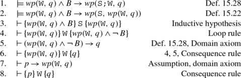
15.7 Summary

Computer programs are similar to logical formulas in that they are formally defined by syntax and semantics. Given a program and two correctness formulas—the precondition and the postcondition—we aim to verify the program by proving: if the input to the program satisfies the precondition, then the output of the program will satisfy the postcondition. Ideally, we should perform program synthesis: start with the pre- and postconditions and derive the program from these logical formulas.

The deductive system Hoare Logic $HL$ is sound and relatively complete for verifying sequential programs in a programming language that contains assignment statements and the control structures if and while.

15.8 Further Reading

Gries (1981) is the classic textbook on the verification of sequential programs; it emphasizes program synthesis. Manna (1974) includes a chapter on program verification, including the verification of programs written as flowcharts (the formalism originally used by Robert W. Floyd). The theory of program verification can be found in Apt et al. (2009), which also treats deductive verification of concurrent programs.

SPARK is a software system that supports the verification of programs; an open-source version can be obtained from http://libre.adacore.com/ .

15.9 Exercises

15.1

What is $wp(\textup {\texttt {S}},\:\mathit{true})$ for any statement S?

15.2

Let S1 be x=x+y and S2 be y=x*y. What is $wp(\textup {\texttt {S1 S2}},\:x < y)$?

15.3

Prove ⊨wp(S, p∧q)→wp(S, p)∧wp(S, q), (the converse direction of Theorem 15.30).

15.4

Prove that

$$\begin{array}{l} \mathit {wp}(\textup {\texttt {if (B) \{ S1 S3 \} else \{ S2 S3 \}}},\,q)=\\ \mathit {wp}(\textup {\texttt {\{if (B) S1 else S2\}\ S3}},\,q). \end{array} $$

15.5

* Suppose that wp(S, q) is defined as the weakest formula p that ensures total correctness of S, that is, if S is started in a state in which p is true, then it will terminate in a state in which q is true. Show that under this definition ⊨¬ wp(S, ¬ q)≡wp(S, q) and ⊨wp(S, p)∨wp(S, q)≡wp(S, p∨q).

15.6

Complete the proofs of the soundness and completeness of $HL$ for the alternative rule (Theorems 15.39 and 15.40).

15.7

Prove the partial correctness of the following program.

15.8

Prove the partial correctness of the following program.

15.9

Prove the partial correctness of the following program.

15.10

Prove the partial correctness of the following program.

15.11

Prove the partial correctness of the following program.

References

K.R. Apt, F.S. de Boer, and E.-R. Olderog. Verification of Sequential and Concurrent Programs (Third Edition). Springer, London, 2009.
D. Gries. The Science of Programming. Springer, New York, NY, 1981.
C.A.R. Hoare. An axiomatic basis for computer programming. Communications of the ACM, 12(10): 576–580, 583, 1969.
Z. Manna. Mathematical Theory of Computation. McGraw-Hill, New York, NY, 1974. Reprinted by Dover, 2003.
Author information
Authors and Affiliations
Rights and permissions
Copyright information
© 2012 Springer-Verlag London
About this chapter
Cite this chapter
Ben-Ari, M. (2012). Verification of Sequential Programs. In: Mathematical Logic for Computer Science. Springer, London. https://doi.org/10.1007/978-1-4471-4129-7_15
Download citation
DOI: https://doi.org/10.1007/978-1-4471-4129-7_15
Publisher Name: Springer, London
Print ISBN: 978-1-4471-4128-0
Online ISBN: 978-1-4471-4129-7
eBook Packages: Computer ScienceComputer Science (R0)