
Abstract
In this chapter, first, reliability is defined. Then, different ways of modeling reliability are discussed. Empirical models are based on field data and are easy to use. Physical models address a certain failure mechanism and are used to predict wearout. Physical models may be either analytical or they may be run by computer simulations. Other useful information on reliability may be obtained by testing either test vehicles or entire products. Comparing the test results with the test results obtained, when testing similar items with field data, gives a quite good idea on which kind of field reliability performance should be anticipated. Interconnection reliability must also be taken into account when checking the reliability of a component. Many times, the actual component may not represent a large risk, whereas solder interconnection may create risks that need to be mitigated. In the end of this chapter, some statistical distributions are discussed. Especially, practical advice on how to use Weibull distribution is revealed.
Access provided by Autonomous University of Puebla. Download chapter PDF
Keywords
These keywords were added by machine and not by the authors. This process is experimental and the keywords may be updated as the learning algorithm improves.
2.1 The Definition of Reliability
Reliability may be defined in several ways. The definition to be used here is the commonly used definition adapted from [1]:
Reliability is the probability that an item operating under stated conditions will survive for a stated period of time.
The above definition has its roots in military handbook MIL-STD-721C [2] and is valid for nonrepairable hardware items. The “item” may be a component, a subsystem, or a system. If the item is software instead of hardware, the definition will be somewhat different [3].
2.2 Empirical Models
Component-level reliability analysis conventions have their background in the military and space industries. As the components used in these applications were clearly safety critical, it was necessary to create qualification criteria and reliability prediction methods [4]. These reliability prediction models were typically based on large field failure databases. The empirical models give a generic estimate for a certain component or technology. Although also being based on empirical data, the effect of field environment was taken into account by “factors” responsible for the degradation effects related to temperature, voltage, or some other stress factor. The temperature dependence was taken into account by the so-called Arrhenius equation [5] that was originally developed when modeling the rate of chemical reactions.
However, although since the early 1970s the failure rates for micro devices have fallen approximately 50% every 3 years [6] and the handbook models were updated on the average every 6 years, the models became overly pessimistic. Finally, in 1994, the US Military Specifications and Standards Reform initiative led to the cancellation of many military specifications and standards [7]. This, coupled with the fact that the Air Force had redirected the mission of the Air Force Research Laboratory (the preparing activity for MILHDBK-217) away from reliability, resulted in MIL-HDBK-217 becoming obsolete, with no government plans to update it.
The cancellation of MIL-HDBK-217 was by no means the end of empirical models. Several similar kind of handbooks still exist, such as Bellcore Reliability Prediction Procedure [8], Nippon Telegraph and Telephone (NTT) procedure [9], British Telecom Handbook [10], CNET procedure [11], and Siemens procedure [12]. The predicted failure rates originating from different standards may, however, deviate from each other [13]. Empirical models can, in principle, also take into account early failures and random failures, which is not usually the case when considering physical models. Empirical models are also easy to use.
2.3 Physical Models
Each physical model [14, 15] is created to explain a specific failure mechanism. First, the testing is performed, the failed samples are analyzed, and the root cause for the failures is discovered [16]. Then, a suitable theory that would explain the specific failure mechanism is selected and used to calculate the acceleration factor and the predicted meantime-to-failure (MTTF) value. This means, that the acceleration factor relevant to the failure mechanism is not usually known prior to the testing and analysis of the root cause.
Physical modeling may be based either on an analytical model or on finite element analysis (FEA) simulations. Physical models are most widely applied in solder joint fatigue modeling. Some other phenomena that have been studied by physical models are electromigration [17], and other thermally induced failure mechanisms [18]. When applying physical models, it is possible to study the effects of material properties, dimensions, and field environment. The problem lies in the large parameter sensitivity of these models. Many models are applying exponential or power equations. The generic solutions to second-order differential equations, usually solved by running FEA simulations, are of exponential type. Therefore, even slightly inaccurate parameter values may result in tremendous errors. Despite this fact, proper error estimates are given far too seldom, although some examples of this do exist [19, 20].
Another aspect that may possibly degrade the level of confidence toward predictions based on physical models is the fact that the models are developed in a well-controlled laboratory environment and there is little reliability data originated in a real field environment [21]. Presently, there are still situations in which no model that would explain the failure mechanism encountered can be found. In those cases, no prediction based on physical models can be given. Physical models usually address to wearout phenomena and, therefore, are of little value if early failures or random failures are in question. The exception to this is overstress events that can be analyzed by stress–strength analysis. Also, methods to assess early failures of defective subpopulations are being developed [22].
2.4 Reliability Information
As discussed earlier in this chapter, there are different ways to estimate the reliability of microsystem components. In order to be able to evaluate the usefulness of such estimates, there should be some key criteria selected for this. One key issue is how much we can rely on the reliability data. Reliability prediction with no correlation to the actual field performance is of little value. It is also vital that the data are available at times when it is useful. After its service life, it is possible, at least in theory, to know exactly the reliability performance of a certain component population. However, this information may not be very useful, as the components have already failed and there is no means anymore to affect the retrofit costs. Therefore, timely information that is based on the best knowledge available would be most desirable for the majority of engineering purposes.
In Fig. 2.1, some reliability information sources are judged based on the two aforementioned criteria: the level of confidence on the reliability information and the time span when the information is available. The graph may be somewhat subjective but should still be quite illustrative. The ranking of the methods based on the level of confidence may be open for discussion. The term “level of confidence” is used here loosely to describe how accurate or trustworthy the information is. Level of confidence should not be confused with the confidence limits or confidence intervals that have exact definitions in statistics.

Reliability information sources: the level of confidence of the information and the time when the information is available
When a component is selected for use in a design, the first indication of its reliability can be based on similar item data. If a similar component has already been used for several years, it is probable that in-house field failure databases can estimate the forthcoming reliability of the introduced component. If the component has not been utilized in a similar product, it is still possible to obtain some generic estimate of its reliability based on the handbooks discussed earlier. However, it should be noted that such information might be based on out-of-date data.
If there is no field data available, physical modeling may also give an initial estimate. Physical modeling is comprised of the utilization of a suitable analytical model and/or a computer simulation analysis. As physical modeling without calibration information may not be very accurate, it is expected that in-house field data in the initial phase would be superior to physical predictions in terms of level of confidence. However, if the generic handbook values are based on old data, the physical models may give a more accurate lifetime prediction.
Only after the reliability testing has been performed is it possible to improve the quality of reliability predictions. The physical models can utilize the test results as an input (calibration data). After this, a more accurate lifetime prediction for the component can be obtained. Moreover, after the test has been concluded, it is possible to compare the test results of the component to similar items that have been tested in the same way and whose field failure data are available. This enables the reliability prediction to be based on concrete data; if the component has performed in the same way as the reference item, it is also probable that the component studied will have approximately similar field reliability behavior. If the component has performed worse than the item on which field data exist, it is expected that the field reliability performance will be somewhat worse than the reference, and vice versa.
The test itself also gives valuable information. If some early failures occur in a test it is a clear signal that there will most likely be early failures in the field as well. This is very important information, which may be very difficult to obtain unless one actually tests the component. Physical models usually predict the wearout of the components only and, therefore, may be of little value when it comes to predicting early failures. The exception to this is overstress events that can be analyzed by stress–strength analysis. Empirical models may be better at taking early failures into account. However, currently, they are not updated very often and, therefore, may be either pessimistic or they may not contain information on the new component type at all.
The shape of the test data curve resembles the bathtub curve used commonly within the reliability community. The early-failure, random-failure, and wearout regions are easily recognizable. However, as the level of confidence – instead of hazard rate – is the parameter monitored, it is expected that the shape of the curve deviates somewhat from the conventional bathtub curve. The occurrence of early failures in a test environment is a relatively reliable indicator that real concerns in the field environment are likely to take place. As the test continues, and failures occur, it may be more difficult to predict if these failures are going to be induced also by the real environment during the life span of the component. The random-failure region obtains a relatively small level of confidence value as it is expected that only a minor share of component population is going to fail during this period of time. After wearout phenomena start to occur, the confidence level is expected to rise again. This time, the level of confidence is, however, less than in case of early failures, as more time has elapsed since the test started. Therefore, it is more difficult to estimate if failures due to wearout are going to be recorded during the life span of the component.
Despite the lack of information on early failures, many times they are responsible for the majority of field failures. This is especially true when it comes to consumer products, whose expected lifetime of use is limited, and therefore, wearing out of components is not very probable. Early failures are due to design bugs, manufacturing faults, and quality problems. After the early-failure period in testing, there is usually a period of time, during which not many failures occur. This is often called the “random failure” section of the bathtub curve. As only a minor share of the equipment fail during this period, the level of confidence is usually low due to the limited number of failure observations. In order to gain an acceptable level of confidence, thousands of items should be tested [23]. This is, however, in conflict with the number of test items usually available and the limited test resources.
As discussed earlier, the information on the wearout period during the test can be used as input data for other prediction methods. After the product has been launched in the field, field failure data starts to accumulate. Ideally, field data would be the most accurate source of reliability information. Unfortunately, the field data may not always be very useful for reliability engineers. There are several reasons for this. The failure analysis is not always thoroughly performed. This is due to the fact that the primary interest of the repair personnel is to repair the product, not to analyze the cause of failure. The field data also contains some failures that are not actually due to the inherent reliability level of the components.
These failures include, for example, misuse of the product. Of course even this kind of information may be valuable, if it is considered that improving the durability of the product is needed. Also, the load history of the failed component is usually lacking, which makes it difficult to understand how the failure was actually initiated. Despite these words of caution, much can be gained if field failure data are utilized effectively. If constantly monitored, the field failure data can provide useful information on subjects of improvement. Improvements based on field data can usually be implemented during the lifetime of the product. However, field data are valid only for a limited time. Technological advances are mostly responsible for this. It may be that the reliability performance of the component improves very much when the technology gets more mature. This has occurred in conjunction with integrated circuit technology, where constant improvements take place. According to MILHDBK-217 version A, a 64-kB RAM would fail in 13 s [24].
This very pessimistic prediction is a most unfavorable example of empirical models. Nowadays, the RAM capacity is several thousand times larger than in the example given, and still, RAMs are not considered as reliability concerns. Another cause for field failure data becoming obsolete is the fact that components and component technologies have a natural life span. Due to the technology-obsolescence cycle, technologies will be replaced by some other technologies, and therefore, reliability estimates using the old technologies are of no interest.
Figure 2.2 shows a new interpretation of stress–strength distribution of a product population. The overlapping part describes the probability for the product failures and the strength of the product will gradually degrade (aging).

New interpretation of stress–strength distribution of a product population
Figure 2.3 shows a typical approach to product total failure estimates in time, with constant component hazard rate. The failures are based on randomly failed individual products that could be a result of quality variation within the product population. It gives somewhat adequate estimates of product failures, especially when the product component set is based on mature technology, the usage environment will be quite the same, and the stress levels do not exceed the strength of the product. In order to make reasonable credible predictions, the new system must be similar to well known existing system without involving significant technological risks.

Product failures- in-time (FIT) caused by components with constant hazard rate
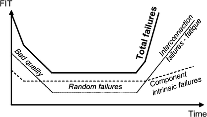
However, if any of the components hazard rates starts to increase during the design lifetime of the product, the constant hazard rate approach is not relevant anymore. In practice, the total hazard rate is a sum of a time-independent constant hazard rate and a time-dependent increasing hazard rate with infant mortality region included. So the product hazard rate would look more like the so-called bathtub curve shown in Fig. 2.4. The component intrinsic failures will increase in time, which will increase the hazard rate. If the total product hazard rate is presented, the other failure modes, e.g., the interconnection failures, should be included. This addition increases the hazard rate even further.

Product failures- in-time (FIT) caused by component intrinsic and interconnection failures. Material and system aging mechanisms are involved
2.5 Interconnection Reliability
In this section, interconnection reliability theories are introduced. The general reliability theories are utilized for this. Figure 2.5 shows different approaches to component reliability, where the component intrinsic and its second-level elements are shown. Approach 1 is the most often used approach, where only the component intrinsic failures are taken into account. These failures include the failures at an IC level as well as a component packaging level.

A diagram representation of different approaches (1–3) of component reliability, divided to component intrinsic (R component intrinsic) and its second-level interconnection elements (R int). O and M denote to the amount of elements to work to maintain the functionality of the system
Approach 1 does not cover the failures caused by second level interconnections, namely, the solder joints or mechanically pressed joints. This approach is relevant for components with robust interconnections. In such systems, the reliability of a component, R, is written simply as:
where R component is an intrinsic reliability of the component.
Approach 2 takes into account the reliability of the second level interconnections. This approach is applicable for components whose second level interconnections are one of the main failure sources. The reliability equation for a component is then written:
where R interconnection is the reliability of the second level interconnections of the component.
Approach 3 is based on Approach 2, but a redundancy of the interconnection elements is shown in detail. This is usually the case with many current component technologies, e.g., processors, where the supply voltage and ground are divided into many subnets. This is done to ensure the thermal and the electrical stability of a component. In spite of that, the most important interconnections, the signal inputs and outputs, do not usually have redundancy. The reliability function of a nonredundant interconnection element of Approach 3 is written as:
where M is the number of the interconnections, R i,interconnection is a reliability of particular nonredundant interconnection element. The redundant part of Approach 3, where the interconnection elements are in parallel, can mathematically be described as:
where M is the amount of parallel interconnection and R i,redundant_interconnection is the reliability of each redundant interconnection element. In the redundant solder joint system, there are multiple joints that have the same function in the system to improve the long-term stability and reliability of the system. In such systems, there is M pieces of interconnections of which a fraction of interconnections, denoted as O, must work to maintain the function of the system. This is referred to as an M-modular redundant system, which can mathematically be described as:
where R interconnection is the reliability of each interconnection element. In practice, every solder joint has its individual failure expectation, which would make the reliability calculation very complex in the M-module redundant systems. In spite of that, (2.5) gives more realistic reliability expectations for redundant systems than the conservative reliability equations for interconnection elements. Figure 2.6 shows the reliability of a redundant system as a function of reliability of each interconnection element, by using (2.5). There are ten solder joints in parallel. To achieve 90% reliability in the solder joint system, when two out of the ten solder joints must work to maintain the function of whole system, the reliability of one solder joint should be at least 34%. With the eight out of ten scenarios, the reliability of each solder joint should be at least 88%. As a reference, when ten solder joints are in series with respect to the reliability, a 98.95% reliability of each solder joint would be needed for 90% overall reliability.

Reliability of a redundant interconnection system as a function of the reliability of the interconnection elements. The interconnection system has ten interconnection elements in parallel, of which a fraction must work to maintain the function of the whole system. 2/10, 4/10, 6/10, and 8/10 fractions are shown
2.6 The Levels of Interconnections
There are numerous failure mechanisms involved in electronic systems, which can be roughly divided into hardware- and software-related failures and failure mechanisms. The hardware failure mechanisms are numerous, where one of the most common hardware failure mechanisms is related to component failure. Furthermore, the component failures could be divided into component intrinsic and component interconnection (extrinsic) failures.
Microsystems are made of different levels of components or subassemblies and their connections to each other. The amount of connections reduces when getting closer to the system level, as can be seen from Table 2.1. A closer look would result in about 1010 subelements and interconnections within a typical digital electronic system. In practice, it would be impossible to accurately predict the reliability of such systems in every packaging and interconnection hierarchy level. Despite that, the total reliability concept should consist of every reliability element of the system. Here the emphasis is on the second level interconnections, and in more detail in the solder joints.
The typical solder joint count in a digital electronics board is between 104 and 105. Failure in any of the solder joints will degrade the functionality of the product or in the worst case stop its function entirely. So there are up to 105 failing elements in the digital product, which are usually left out of the risk analyses. In the most straightforward designs, where no redundancy is used, the failure in any of the components or their connections will lead instantly to system failure. In current electronic devices, this vulnerability has been taken into account, and enough redundancy has been applied to maintain the product function at least for the designed lifetime.
Interconnection reliability analysis has not been a solid part of the product reliability concept. This is mainly due to the interconnection technologies and the set of components used in the through-hole and early surface mount technology era. Mainly in the 1970s to 1990s, the interconnection failures were not the main cause of the product failures. This can be verified from the MIL-HDBK-217F (1991), where the empirical data-based solder joint base hazard rates are given by 41 failures per 1012 h for through-hole assemblies and 69 failures per 1012 h for reflow solder joints. To put this in perspective, the hazard rates are roughly a thousand times lower than the typical component intrinsic failures for current processors. This is due to the stress-relieving leads together with relative high volume of solder and wide contact areas between lead and solder.
With the emphasis on miniaturization of the products, the components and their interconnections are getting smaller. This will lead inevitably to a situation where the interconnection failures will be playing a more significant role in product failures. New technologies are evolving continuously, and the product design time is getting shorter. Furthermore, new technologies that do not have field experience are taken in to the new product designs with accelerating pace. New technology implementation will usually mean an advantage in respect of the competitors and value adding to the customers. In order to gain the trust to the new technology, powerful and user-friendly applications for failure estimates must be taken into use. Ignoring the importance of the second-level interconnections would potentially result in catastrophic field performance at least in the very harsh usage environment and with so-called long-life high-reliability microsystems.
The standard surface mount components, which are being manufactured under standardized and mature process steps, have been in use for the past two decades. Despite the long experience of these components, their solder joint reliability performance has not been monitored under any specified or standardized procedure. With the ever increasing overall requirements for the electronics, the standard components may also become very risky. This development increases the need for a total reliability concept, where the interconnection elements are taken into account. This is emphasized with the higher risk component packages.
Before one can interpret reliability data in the literature, or compare results from different sources, it is necessary to develop a formal framework of reliability theory and definitions.
2.7 Reliability Function
Let us denote F(t) to be the failure function. Then the reliability function is:
Let us look at a simple test: we have 1,000 flip-chip joints. After 10 h, 103 joints are broken. Then the failure function is F(t) = 103/1,000 = 0.103 = 10.3% at 10 h. At 20 h, an additional 72 joints fail and so forth. We can then plot the failure function as shown in Fig. 2.7, where the last joint failed at 400 h.

Cumulative failure function [25]
Then the failure probability density function (PDF) is:
We can also define a complementary “unreliability” function Q(t), given by:
so from the failure PDF equation above:
and,
i.e., the “unreliability” Q(t) is actually the cumulative failure function F(t). Similarly:
and,
In many cases, the hazard rate λ(t) (sometimes termed the force of mortality) is more useful, or more convenient to use, than the failure PDF f(t). The hazard rate is the failure rate normalized to the number of surviving operational parts, i.e.,
from which we can readily relate the hazard rate λ(t) to the failure PDF f(t) by:
and determine the cumulative hazard rate H(t), [analogous to the cumulative failure function F(t)], to be:
since R(0) = 1.
Another commonly used reliability criterion is the mean time to failure (MTTF), defined as:
which reduces to:
after integration by parts, and provided that R(t) → 0 for t ≪ ∞.
These results and relationships are summarized for convenience in Table 2.2, which also includes additional information developed below. The example of a cumulative failure function shown in Fig. 2.8 corresponds to the bottom bathtub curve of Fig. 2.9.

Cumulative failure function

Bathtub curve changes with increased stress (e.g., temperature, voltage, etc.)
2.7.1 Exponential Distribution
The simplest practical failure PDF, and one with wide application in electronics, is the single parameter exponential distribution function:
where u(t) is the Heaviside step function [u(t) = 0 for t < 0, and u(t) = 1 for t > 0] and λ 0 is called the chance hazard rate. Applying the formula above:
Similarly, the hazard rate, λ e (t), and MTTF are given by:
and,
respectively, which suggest the interpretation of reliability as:
Note that the constant hazard rate result does not equate to the constant failure rate at the bottom of the bathtub curve, but there can be a functional approximate equivalence:
where n f (t) have failed and n s(t) survived at time t of sample size n 0, if n s (t) ≈ n 0, i.e., if most of the original sample survives.
In plotting failure data to determine the specific parameter (or parameters) to characterize the specific component set, one counts the failures as a function of time, and the accumulated (total number) of failures, Q(t), and uses the cumulative hazard rate, H(t), in the form:
For the exponential distribution, with Q e (t) = 1 − exp(−λt), the slope of the log-linear plot of 1/(1 − Q(t)) vs. t (which necessarily passes through the origin) gives λ = MTTF −1 (Fig. 2.10), from:

Exponential distribution: Schematic semilog plot
There is usually such an implicit assumption made of which mathematical distribution would apply in deciding how to plot the failure data (and hence implicitly of the failure mechanism).
2.7.2 Weibull Distribution
In fact, the exponential distribution is a special single parameter case of the more general three-parameter Weibull distribution:
which yields reliability:
The effects of shape parameter/factor β, scale parameter/factor η, and location parameter/factor γ, are shown in Fig. 2.11, with the Weibull hazard rate and cumulative hazard rate variations with shape factor illustrated in Fig. 2.12.

Weibull distribution: failure probability density function (PDF). (a) Effect of shape parameter β(γ = 0, η = 1); (b) Effect of scale parameter η(γ = 0, β = 2); (c) Effect of location parameter γ(η = 1, β = 2)

Weibull distribution: Effect of shape factor β (γ = 0, η = 1)
For the shape factor (β > 0):
-
β < 1 represents early failure (including burn-in)
-
β = 1 represents constant failure rate (e.g., the bottom of the bathtub curve)
-
β > 1 represents the wearout phase
For the location parameter, γ:
-
γ < 0 covers a preexisting failure condition before t = 0, e.g., from storage, transport, etc.
-
γ = 0 represents the usual condition where failure begins at t = 0
-
γ > 0 applies when there is a failure-free period until t = γ (Note that the symbol α is often used instead of η for the scale factor.)
For the usual case, where γ = 0, the three-parameter Weibull distribution reduces to the two-parameter Weibull distribution, which then reduces further to the exponential distribution above with β = 1 and η = 1/λ 0 (see Figs. 2.11a and 2.12); Note from Fig. 2.12 that β = 0.5, 1, and 3 can be seen as representative of the early failure, constant failure phase, and wearout sections of the bathtub curve, respectively (provided that n f < n 0, as explained above).
Again, the cumulative hazard rate, for Q w(t) = 1 − exp−(t/η)β, gives:
so, to find both β and η, one plots log{log[1/(1 − Q(t))]} vs. log t, and gets η from the intercept, and β from the slope (Fig. 2.13), as:

Weibull distribution: Schematic plot
and Weibull log.log vs. log graph paper is available to facilitate direct plotting.
Table 2.2 includes a summary of the Weibull and exponential distributions, and of the Rayleigh distribution, which is specified by γ = 0, and β = 2, where \( \eta = \sqrt {2/k} \).
In the context of the location parameter, it is worth noting that the assignment of t = 0 is clearly arbitrary, and we can define a conditional reliability, R(t, T), as the probability of the (nonrepairable) device or system to operate for time, t, having already operated for time, T, as:
2.7.3 Log-Normal Distribution
The other failure probability distribution with significance in microelectronics is the log-normal, given by:
where z = (ln t − μ)/σ, μ = ln T 50, and T 50 is defined as the time t f at which Q LN(t f) = R LN(t f) = 0.5 or 50%. Re-writing the expression for z:
where Φ−1(Q LN(t)) is a tabulated function of Q LN(t). This equation can be plotted readily on log-normal graph paper, where the log(time-to-failure) x-axis is labeled in terms of time, and the y-axis (which is actually Φ−1(Q LN(t))) is labeled as the cumulative failed percentage (or failure probability), Q(t). (Figure 2.14 shows such a plot, but with the axes reversed to match the form of the equation above. Since z = 0 at t = T 50, Q = 50%, and z = −1 at t = T 15.9, Q = 15.9%, the slope of this plot gives slope = σ = ln(T 50/T 15.9).) The log-normal parameters f LN(t), λ LN(t), and Q LN(t), are shown for completeness as functions of time in Fig. 2.15, with T 50 = eμ as the third parameter.

Log-normal distribution: Schematic plot

Log-normal distribution: schematic plots of distribution parameters (failure PDF, hazard rate, and cumulative failures) vs. time
2.7.4 Physical Basis of the Distributions
For β = 1, the Weibull distribution reduces to the exponential, with λ = constant = λ 0, corresponding to the bottom of the bathtub curve. In modern electronic systems, the apparently constant hazard rate actually masks many different and unrelated failure modes with different temporal rates. In this case, any attempt to model these varied physical failure processes with a single parameter set, as if they were all due to the same failure mechanism, would clearly be flawed. In particular, if one then tried to apply a single formula for thermal variation of these many different physical processes to predict failure rates under other circumstances, the results would be unlikely to match reality. This was the fundamental problem when Military Handbook Standard 217, which was developed to model and predict single constant hazard rate failure modes, began to be applied to the apparently constant rate of modern complex systems, which result from low random failure rates from diverse causes. For the Rayleigh distribution, where β = 2, λ(t) is directly proportional to t, and clearly this case corresponds to failure due to time-accumulated damage.
Where only one defect site causes the failures, and the damage susceptible population is removed, λ(t) decreases as time goes on, and corresponds to the early failure (burn-in) section of the bathtub curve, e.g., for the Weibull distribution with β = 0.5.
A log-normal distribution can arise in the following way, if failure occurs when a resistance, r, increases to the failure threshold r n . Assume that the resistance increases with each time step as r i+1 = r i (1 + δ) from the initial value r 0, then:
where δ i is an independently distributed random variable, and hence, log r n is normally distributed and r n (the end of life resistance) is log-normally distributed.
One might expect that at least the general nature of the physical origin of reliability failures might be determined by the fit or otherwise of the data to the distribution assumed for the graphical plots. However, the Weibull and log-normal plots of the same data shown in Fig. 2.16 demonstrate that the fit can be ambiguous.


2.8 A Generic Weibull Distribution Model to Predict Reliability of Microsystems
The classic two-parameter Weibull distribution has the following form:
Then the failure intensity function is in this case:
The traditional three-parameter Weibull distribution has the following form:
where α is the scale parameter, β is the shape parameter, which is a kind of wear characteristic or associated with different failure modes, and τ is the location parameter indicating the minimum life.
2.8.1 Failure-Criteria Dependence of the Location Parameter
Since α and β in the Weibull distribution are material dependent with α characterizing the strength of the material and β characterizing the aging effect of the material, it can be assumed that they are independent of the failure criterion in this case. However, the location parameter τ should depend on the failure criterion because of the cumulative damage leading to a failure. A new 4-parameter Weibull distribution is described below. The new distribution is able to handle the resistivity change as a failure criterion. We demonstrate this by looking into the reliability of anisotropic conductive adhesive joints.
Let the failure criterion be generally described as r > kr 0, where r 0 is the nominal level.
Let τ 0 be the location parameter at the nominal value. Here we assume that this location parameter τ 0 is greater than 0, which means that the material has a failure-free life until τ 0. Some preliminary analysis indicates that a model for τ could be:
where b is an empirical parameter to be estimated with test data. That is, the probability of failure at time t depends on the value of k in the following manner:
Hence, this is a model with four parameters, but it can be fitted to the datasets under different criteria at the same time. Such a model is useful in many aspects. Some are discussed in the following.
First, the minimum life defined as τ = τ 0 k b can be computed for any given failure criterion. This provides a theoretical explanation of the existence of the minimum life and its dependence of the failure criteria.
Second, fixing a minimum cycle time to failure, the failure criterion that meets this requirement can be determined. This is useful in a contractual situation when a minimum cycle time is to be guaranteed. That is, if the required or guaranteed minimum cycle life is τ r, from the inequality τ 0 k b ≥ τ r, we get that k ≥ (τ r/τ 0)1/b. In other words, the failure criteria can at least be set as k = (τ r/τ 0)1/b.
Furthermore, under any failure criterion, the cumulative failure probability can be computed at any time.
2.8.2 Least Squares Estimation
The general model contains four parameters that have to be estimated using the data from testing. Various methods can be used, and here the parameters can be estimated by a simple least square method. Here the cumulative distribution function is estimated by the mean ranking with the form:
and the sum of square deviation can be written as:
where m different failure criteria have been considered and n i samples are tested for each criterion i and k i is the criterion parameter of criterion i. For each sample group with n i samples, d i components have failed, and t ij is the time to failure for the jth failed component.
Since parameter τ 0 is defined as the location parameter at the nominal failure criterion, it is suggested to use the sample data under the nominal failure criterion to estimate the parameter τ 0.
Therefore, the minimization of SSE is accomplished by taking the partial derivatives of SSE with respect to the parameters and setting the resulting equations to zero, which leads to:
and,
The above equations can be solved using a computer spreadsheet or software. Also note that the location parameter model τ i = τ 0 k b should satisfy the condition that τ i ≤ τ i1 under each failure criterion i.
2.8.3 The Experiment and Data
The general approach above is verified for the analysis of conductive adhesive joining in flip-chip packaging.
A significant number of accelerated reliability tests under well-controlled conditions based on single joint resistance measurement to generate significant reliability data for using anisotropic conductive adhesive (ACA) flip-chip technology on FR-4 substrate have been generated in the literature [26]. Nine types of ACA and one nonconductive film (NCF) were used. In total, nearly one thousand single joints were subjected to reliability tests in terms of temperature cycling between −40 and 125°C with a dwell time of 15 min and a ramp rate of 110°C/min. The chip used for this reliability test had a pitch of 100 μm. Therefore, the test was particularly focused on evaluation of the reliability of ultrafine pitch flip-chip interconnections using ACA on a low-cost substrate.
The reliability was characterized by single contact resistance measured using the four-probe method during temperature cycling testing up to 3,000 cycles. The failure definitions are defined as 20% increase, larger than 50 mΩ, and larger than 100 mΩ, respectively, using the in situ electrical resistance measurement technique. Usually when tests are carried out in different conditions or when the data are from different failure criteria, the datasets are analyzed separately. This usually involves a large number of combined model parameters, and there is no clear relationship between the model parameters.
The test setup: To study the reliability of conductive adhesive joints, contact resistance of single joints is one of the most important parameters. Therefore, a test chip was designed for four-probe measurement of single joints. The configuration of the test chip contains 18 single joints and two daisy chains (18 joints for each). The pitch of the test chips is 100 μm. Bump metallization of the chips is electroless nickel and gold. Table 2.3 summarizes some characteristic parameters of the test chip. Here the reliability study focused on the reliability of ACA joining, i.e., the characteristics of ACA joints together with the usage environment. A temperature cycling test was applied for the evaluation. The reliability of ACA joints was characterized by the change of contact resistance in the cycled temperatures. A total of 954 joints (53 chips) with different ACA materials were tested. Two chips with 36 joints were measured in situ with the four-probe method during testing up to 3,000 cycles, and other joints were taken out from the equipment every several hundred cycles to manually measure the resistance change in room temperature.
Most ACA joints were manually measured every several hundred cycles because of the capacity of the cabinet. A total of 918 joints (51 chips) were tested. Some of them, 126 joints of 7 chips, failed after only 200 cycles due to bad alignment, so they were screened out. The remaining 792 joints (44 chips) were tested for 1,000 cycles. Cumulative failures of the ACA flip-chip joints were measured manually at room temperature. According to different criteria (i.e., the resistance increase was over 20%, contact resistance was over 50 and 100 mΩ).
Test results and discussions: Cumulative fails of the in situ testing are shown in Fig. 2.17. The number of fails is dependent on the definition of the failure. Figure 2.18 shows three statistics on the cumulative fails respectively based on the different criteria: >20% of contact resistance increase; >50 mΩ; >100 mΩ. When the criterion was defined at 20% of resistance increase, after 2,000 cycles all joints had failed. This definition might be too harsh for those joints only having a contact resistance of several mΩ. The 20% increase means only a few milliohms is allowed to vary. In some case, the limitation is still within the margin of error of the measurement.

Cumulative failure plot during temperature cycling test

A typical trend of resistance change as a function of the number of cycles
If we, in any case, allow 50 or 100 mΩ as the failure criteria, we will obtain a MTTF value of 2,500 and 3,500 cycles respectively from a simple Weibull probability plot. Therefore, it is reasonable that the criterion is defined according to the production requirements.
A problem in the analysis of this type of data is that failures under different criteria are usually analyzed separately. With a small number of data points and a large total number of model parameters, the analysis is usually inaccurate. It would be useful to develop an approach for joint analysis of the datasets. The following sections present a Weibull model with the analysis of the data in Fig. 2.18 as an example.
2.8.4 Analysis and the Results
Here we will follow the general model presented earlier. Data of the failure of adhesive flip-chip joints on an FR-4 substrate during the temperature cycling test are considered to illustrate the above new model and estimation. Under criterion II (failure if resistance >50 mΩ) and criterion III (Table 2.4) (failure if resistance >100 mΩ), the cumulative number of failures are summarized in the following table: The nominal level of the test (r 0) is 6 mΩ, thus the criterion parameters k 1 and k 2 are r 1/r 0 = 50/6 = 8.33 and r 1/r 0 = 100/6 = 16.67 respectively. Using simple spreadsheet, the traditional least square estimation of the parameters is given by:
α = 1,954, β = 4.076, τ 0 = 370, b = 0.409 and SSE = 0.1261.
The overall model is then given by:
where k is the failure criterion in terms of “failure when the resistance is k times the nominal value.” This above formula can be used for different failure criteria.
2.8.5 Application of the Results
From the above analysis, note that the minimum cycle life is given by: Minimum life = 370k 0.409. Hence, for any given failure criterion, we can obtain the minimum life with this formula. The estimated minimum life at failure definition of larger than 50 and 100 mΩ are respectively 880.68 and 1169.33. Table 2.5 shows the estimated minimum life and MTTF under some different failure conditions.
Furthermore, for fixed or agreed cycle to failure, we can obtain the maximum failure criteria as:
that is:
That is, to be sure that the minimum life is c 0, the failure criteria cannot be more stringent that “failure when the resistance is k 0 times the nominal value.” This is, for example, a statement that can be used together with the minimum life requirement and can be added in the contractual situation.
References
F. Jensen, “Electronic Component Reliability, Fundamentals, Modeling, Evaluation, and Assurance”, John Wiley & Sons, New York, 1995.
Military Standard MIL-STD-721C, Definitions for Terms for Reliability and Maintainability, June, 1981.
International Standard, Information technology – Software product quality, Part 1: Quality Model, ISO/IEC FDIS 9126-1, ISO/IEC 2000.
MIL-HDBK-217, Reliability Prediction of Electronic Equipment, Version E, October, 1986, 166.
S. Arrhenius, “On the Reaction Velocity of the Inversion of Cane Sugar by Acids,” Zeitschrift für Physikalische Chemie 4, 1889, 226ff.
D. L. Crook, “Evolution of VLSI Reliability Engineering”, Proc. Int. Reliability Physics Symposium, 1990, 2–11.
W. Perry, “Specifications and Standard – A New Way of Doing Business”, US Department of Defense Policy Memorandum, June, 1994.
TS-TSY-000332, Reliability Prediction Procedure for Electronic Equipment, Issue 2, Bellcore, July, 1988.
Standard Reliability Table for Semiconductor Devices, Nippon Telegraph and Telephone Corporation, March, 1985.
Handbook of Reliability Data for Components Used in Telecommunications Systems, Issue 4, British Telecom, January, 1987.
Recuiel De Donnes De Fiabilite Du CNET (Collection of Reliability Data from CNET), Centre National D’Etudes des Telecommunications (National Center for Telecommunication Studies), 1983.
SN29500, Reliability and Quality Specification Failure Rates of Components, Siemens Standard, 1986.
J. B. Bowles, “A Survey of Reliability-Prediction Procedures for Microelectronic Devices”, IEEE Transactions on Reliability, 41, 1992, 2–12.
CALCE. http://www.calce.umd.edu/
N. Kelkar, A. Fowler, M. Pecht and M. Cooper, “Phenomenological Reliability Modeling of Plastic Encapsulated Microcircuits”, International Journal of Microcircuits and Electronic Packaging, 19(1), 1996, 167.
T. Stadterman, B. Hum, D. Barker and A. Dasgupta, “A Physics-of-Failure Approach to Accelerated Life Testing of Electronic Equipment”, Proc. for the Test Technology Symposium ’96, US Army Test and Evaluation Command, John Hopkins University/Applied Physics Laboratory, 4–6, June, 1996.
J. R. Black, “Physics of Electromigration”, Proc. International Reliability Physics Symposium, 1974, 142–164.
J. Liu, L. Cao, M. Xie, T. N. Goh and Y. Tang, “A General Weibull Model for Reliability Analysis Under Different Failure Criteria – Application on Anisotropic Conductive Adhesive Joining Technology”, IEEE Component Packaging and Manufacturing Technology, 28(4), October 2005, 322–327.
J. P. Clech, “Solder Reliability Solutions, A PC-Based Design-For-Reliability Tool”, Proc. of Surface Mount International, SMTA, San Jose, CA, 1996.
A. Syed, “Predicting Solder Joint Reliability for Thermal, Power and Bend Cycle within 26% Accuracy”, Proc. of the 51st Electronics Components and Technology Conference, Orlando, 2001, 255–263.
J. Galloway, L. Li, R. Dunne and H. Tsubaki, “Analysis of Acceleration Factors Used to Predict BGA Solder Joint Field Life”, Proc. SMTA International, Chicago, 2001, 357–363.
M. S. Moosa and K. F. Poole, “Simulating IC Reliability with Emphasis on Process-Flaw Related Early Failures”, IEEE Transactions on Reliability, 44, 1995, 556–561.
E. Demko, “Commercial-Off-The-Shelf (COTS): A Challenge to Military Equipment Reliability”, Proc. Annual Reliability and Maintainability Symposium, Las Vegas, NV, 1996, 7–12.
T. Ejim, “High Reliability Telecommunications Equipment: A Tall Order for Chip-Scale Packages”, Chip Scale Review, 5, 1998, 44–48.
R. Tummala, “Fundamentals of Microsystems Packaging”, McGraw-Hill Professional, New York, 2001.
M. Ohring, “The Mathematics of Failure and Reliability” in “Reliability and Failure of Electronic Materials and Devices”, Academic Press, San Diego, CA, 1998, 200–201, Chapter 4.
Author information
Authors and Affiliations
Corresponding author
Exercises
Exercises
-
2.1
Explain the curve shown below. What is the reason for failures in the different regions?
-
2.2
Consider the following equation:
$$ {R_{O{/}M}}\,{ =\, 1} - \sum\limits_{{i = 0}}^{O - {1}} {\left\{ {\frac{{M{!}}}{{{(}M - i{)!}i{!}}}} \right\}} R_{\rm{interconnection}}^i{{(1} - {R_{\rm{interconnection}}}{)}^{M - i}}. $$What is the solder joint reliability if seven of ten components work to maintain 90% system reliability? Plot the whole reliability diagram.
-
2.3
Draw the curve of the following equation that shows the failure rate function.
$$ f(t) = \frac{\beta }{\alpha }{\left( {\frac{t}{\alpha }} \right)^{\alpha - 1}}\exp \{ - {[(t)/\alpha ]^\beta }\}. $$What conclusions can you draw from the curve?
-
2.4
The infant mortality and wear out sections of Fig. 2.9 are plotted for the sake of the example as simple cubic functions for t < 200 and t > 800 hours in the bottom curve. (a) Predict when the last component will die. (b) Verify that your result seems sensible by extrapolating the wear out section of Fig. 2.8.
-
2.5
Tables A and B below present failure time data for two sequences of lab experiments, each on 20 samples. (a) Plot the data for both Weibull and log-normal distributions. (b) Determine η and β for the Weibull plot, and σ for the log-normal plot. (c) What is the mean failure time for each? (d) Can you establish the appropriate reliability distribution model from the plots? (e) Compare the data sets, and discuss, noting the regular failure rate in Table A.
Table A
Failure
1
2
3
4
5
6
7
8
9
10
Time(hr)
40
98
150
210
255
295
351
402
445
503
Failure
11
12
13
14
15
16
17
18
19
20
Time(hr)
551
595
648
705
750
790
860
900
950
1008
Table B
Failure
1
2
3
4
5
6
7
8
9
10
Time(hr)
15
35
50
70
90
115
135
160
190
220
Failure
11
12
13
14
15
16
17
18
19
20
Time(hr)
255
290
335
380
440
510
600
730
950
1500

Rights and permissions
Copyright information
© 2011 Springer Science+Business Media, LLC
About this chapter
Cite this chapter
Liu, J., Salmela, O., Särkkä, J., Morris, J.E., Tegehall, PE., Andersson, C. (2011). Reliability Metrology. In: Reliability of Microtechnology. Springer, New York, NY. https://doi.org/10.1007/978-1-4419-5760-3_2
Download citation
DOI: https://doi.org/10.1007/978-1-4419-5760-3_2
Published:
Publisher Name: Springer, New York, NY
Print ISBN: 978-1-4419-5759-7
Online ISBN: 978-1-4419-5760-3
eBook Packages: EngineeringEngineering (R0)