
Abstract
Background
Photovoltaic (PV) array which is composed of modules is considered as the fundamental power conversion unit of a PV generator system. The PV array has nonlinear characteristics and it is quite expensive and takes much time to get the operating curves of PV array under varying operating conditions. In order to overcome these obstacles, common and simple models of solar panel have been developed and integrated to many engineering software including Matlab/Simulink. However, these models are not adequate for application involving hybrid energy system since they need a flexible tuning of some parameters in the system and not easily understandable for readers to use by themselves. Therefore, this paper presents a step-by-step procedure for the simulation of PV cells/modules/arrays with Tag tools in Matlab/Simulink. A DS-100M solar panel is used as reference model. The operation characteristics of PV array are also investigated at a wide range of operating conditions and physical parameters.
Result
The output characteristics curves of the model match the characteristics of DS-100M solar panel. The output power, current and voltage decreases when the solar irradiation reduces from 1000 to 100 W/m2. When the temperature decreases, the output power and voltage increases marginally whereas the output current almost keeps constant. Shunt resistance has significant effect on the operating curves of solar PV array as low power output is recorded if the value of shunt resistance varies from 1000 ohms to 0.1 ohms.
Conclusion
The proposed procedure provides an accurate, reliable and easy-to-tune model of photovoltaic array. Furthermore, it also robust advantageous in investigating the solar PV array operation from different physical parameters (series, shunt resistance, ideality factor, etc.) and working condition ( varying temperature, irradiation and especially partial shadow effect) aspects.
Background
Mathematical modeling of PV module is being continuously updated to enable researchers to have a better understanding of its working. The models differ depending on the types of software researchers used such as C-programming, Excel, Matlab, Simulink or the toolboxes they developed.
A function in Matlab environment has been developed to calculate the current output from data of voltage, solar irradiation and temperature in the study of (Walker 2001) and (Gonzalez-Longatt 2005). Here, the effect of temperature, solar irradiation, and diode quality factor and series resistance is evaluated. A difficulty of this method is to require readers programming skills so it is not easy to follow. Another method which is the combination between Matlab m-file and C-language programming is even more difficult to clarify (Gow and Manning 1999).
Among other authors, a proposed model is based on solar cell and array’s mathematical equations and built with common blocks in Simulink environment in (Salmi et al. 2012), (Panwar and Saini 2012), (Savita Nema and Agnihotri 2010), and (Sudeepika and Khan 2014). In these studies, the effect of environmental conditions (solar insolation and temperature), and physical parameters (diode’s quality factor, series resistance Rs, shunt resistance Rsh, and saturation current, etc.) is investigated. One disadvantage of these papers is lack of presenting simulation procedure so it causes difficulties for readers to follow and simulate by themselves later. This disadvantage is filled in by (Jena et al. 2014), (Pandiarajan and Muthu 2011). A step-by-step procedure for simulating PV module with subsystem blocks with user-friendly icons and dialog in the same approach with Tarak Salmi and Savita Nema is developed by Jena, Pandiarajan and Muthu et al. However, the biggest gap of the studies mentioned above is shortage of considering the effect of partially shading condition on solar PV panel’s operation.
In other researches, authors used empirical data and Lookup Table or Curve Fitting Tool (CFtool) to build P–V and I–V characteristics of solar module (Banu and Istrate 2012). The disadvantage of this method is that it is quite challenging or even unable to collect sufficient data if no experimental system be available so that modeling curves cannot be built and modeled.
From the work of (Ibbini et al. 2014) and (Venkateswarlu and Raju 2013), a solar cell block which has already been built in Simscape/Simulink environment is employed. With this block, the input parameters such as short circuit current, open circuit voltage, etc. is provided by manufacturers. The negative point of this approach is that some parameters including saturation current, temperature, and so on cannot be evaluated.
Solar model developed with Tag tools in Simulink environment is recorded in the research of (Varshney and Tariq 2014), (Mohammed 2011), etc. In these papers, only two aspects (solar irradiation and temperature) are investigated without providing step-by-step simulation procedure.
In overall, although having advantages and disadvantages, different methods have similar gaps as follows:
-
The proposed models are not totally sufficient to study all parameters which can significantly affect to I–V and P–V characteristics of solar PV array, including physical parameters such as saturation current, ideality factor, series and shunt resistance, etc. and environmental working conditions (solar insolation, temperature and especially shading effect).
-
Lack of presenting step-by-step simulation procedure and this causes difficulties for readers and researchers to follow and do simulation by themselves.
Therefore, the study proposes a robust model built with Tag tools in Simulink environment. The proposed model shows strength in investigating all parameters’ influence on solar PV array’s operation. In addition, a unique step-by-step modeling procedure shown allows readers to follow and simulate by themselves to do research.
Methods
Mathematical equivalent circuit for photovoltaic array
The equivalent circuit of a PV cell is shown in Fig. 1. The current source Iph represents the cell photocurrent. Rsh and Rs are the intrinsic shunt and series resistances of the cell, respectively. Usually the value of Rsh is very large and that of Rs is very small, hence they may be neglected to simplify the analysis (Pandiarajan and Muthu 2011). Practically, PV cells are grouped in larger units called PV modules and these modules are connected in series or parallel to create PV arrays which are used to generate electricity in PV generation systems. The equivalent circuit for PV array is shown in Fig. 2.

PV cell equivalent circuit (Salmi et al. 2012)

Equivalent circuit of solar array (Tu and Su 2008)
The voltage–current characteristic equation of a solar cell is provided as (Tu and Su 2008; Salmi et al. 2012): Module photo-current Iph:
Here, Iph: photo-current (A); Isc: short circuit current (A) ; Ki: short-circuit current of cell at 25 °C and 1000 W/m2; T: operating temperature (K); Ir: solar irradiation (W/m2).
Module reverse saturation current Irs:
Here, q: electron charge, = 1.6 × 10⁻¹⁹C; Voc: open circuit voltage (V); Ns: number of cells connected in series; n: the ideality factor of the diode; k: Boltzmann’s constant, = 1.3805 × 10⁻²³ J/K.
The module saturation current I0 varies with the cell temperature, which is given by:
Here, Tr: nominal temperature = 298.15 K; Eg0: band gap energy of the semiconductor, = 1.1 eV; The current output of PV module is:
With
and
Here: Np: number of PV modules connected in parallel; Rs: series resistance (Ω); Rsh: shunt resistance (Ω); Vt: diode thermal voltage (V).
Reference model
The 100 W solar power module is taken as the reference module for simulation and the detailed parameters of module is given in Table 1.
Step by step procedure for modeling of photovoltaic arrays with tags
A mathematical model of PV array including fundamental components of diode, current source, series resistor and parallel resistor is modeled with Tags in Simulink environment (http://mathwork.com). The simulation of solar module is based on equations given in the section above and done in the following steps.
Step 1
Provide input parameters for modeling:
Tr is reference temperature = 298.15 K; n is ideality factor = 1.2; k is Boltzmann constant = 1.3805 × 10⁻²³ J/K; q is electron charge = 1.6 × 10⁻¹⁹; Isc is PV module short circuit current at 25 °C and 1000 W/m2 = 6.11 A; Voc is PV module open circuit voltage at 25 °C and 1000 W/m2 = 0.6 V; Eg0 is the band gap energy for silicon = 1.1 eV. Rs is series resistor, normally the value of this one is very small, = 0.0001 Ω; Rsh is shunt resistor, the value of this is so large, = 1000 Ω (Fig. 3).

Input parameters for simulation model
Step 2
Module photon-current is given in Eq. (1) and modeled as Fig. 4 (Ir0 = 1000 W/m2).
Step 3

Modeled circuit for Eq. (1)
Module reverse saturation current is given in Eq. (2) and modeled as Fig. 5.

Step 4
Module saturation current I0 is given in Eq. (3) and modeled as Fig. 6.

Modeled circuit for Eq. (3)
Step 5
Modeled circuit for Eq. (6) (Fig. 7).

Modeled circuit for Eq. (6)
Step 6
Modeled circuit for Eq. (4) (Fig. 8).

a Modeled circuit for Eq. (4). b Solar subsystem simulation model
Step 7
The solar module simulation procedure is shown from Fig. 3 to Fig. 8b. The solar PV array includes six modules and each module has six solar cells connected in series. Therefore, the proposed model of solar PV array is given in Fig. 9.

Simulation model of solar PV array
Experimental test
In order to validate the Matlab/Simulink model, the PV test system of Fig. 10 is installed. It consists of a rheostat, a solar irradiation meter, two digital multi-meters and a solar system of two DS-100M panels connected in series, each panel has the key specifications listed in Table 1.

Setup of the experimental solar system
Result and discussion
Simulation scenario
With the developed model, the PV array characteristics are estimated as follows.
-
(i)
I–V and P–V characteristics under varying irradiation with constant temperature are given in Fig. 11a and b. Here, the solar irradiation changes with values of 100, 500 and 1000 W/m2 while temperature keeps constant at 25 °C.
Fig. 11 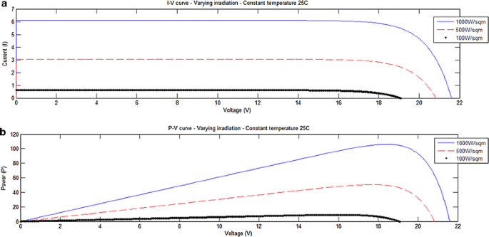
a Output I–V curve with varying irradiation. b Output P–V curve with varying irradiation
Summary when the irradiation increases, the current and voltage output increase. This results in rise in power output in this operating condition.
-
(ii)
I–V and P–V characteristics under varying temperature and constant irradiation are obtained in Fig. 12a and b. Here, the temperature varies from 25 to 50 and 75 °C respectively whereas the irradiation level keeps constant at 1000 W/m2.
Fig. 12 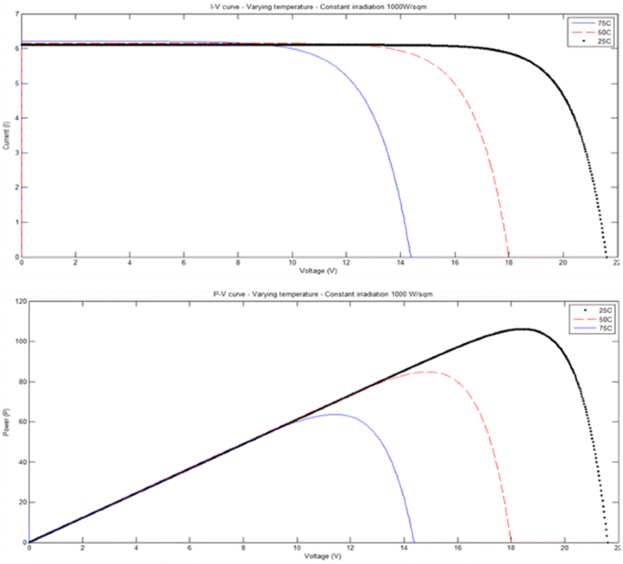
a Output I–V curve with varying temperature. b Output P–V curve with varying temperature
Summary when the operating temperature increases, the current output raises marginally but the voltage output decreases drastically. This leads to net reduction in power output with rise in temperature.
-
(iii)
I–V and P–V characteristics under varying shunt/parallel resistance Rsh, constant temperature and irradiation are shown in Fig. 13a and b. In this case, Rsh changes with three values of 0.1, 1 and 1000 Ω, respectively.
Fig. 13 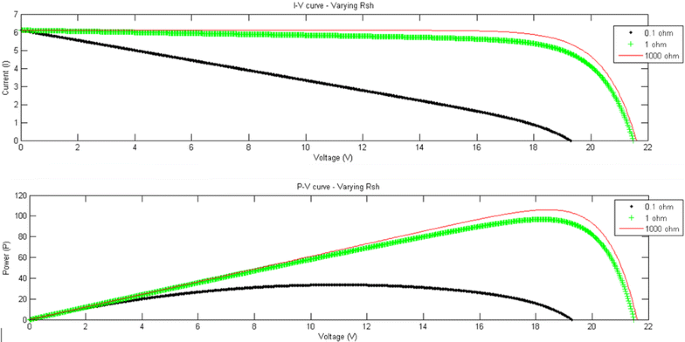
a Output I–V curve with varying Rsh. b Output P–V curve with varying Rsh
Summary when Rsh varies between 1000 and 1 Ω, the current output and voltage output decreases slightly and this results in slight net reduction in power output. However, a significant decrease in current, voltage and power output is recorded when the value of Rsh is 0.1 Ω.
-
(iv)
I–V and P–V characteristics under varying Ns and Np are obtained in Fig. 14a and b. In practice, PV cells are connected in series into PV module and these PV modules then are connected in series or parallel to form PV array for generating more electricity from sunlight. The reference model is 36-series-connected-cell array so two cases are studied: two modules are connected in series and two modules are connected in parallel.
Fig. 14 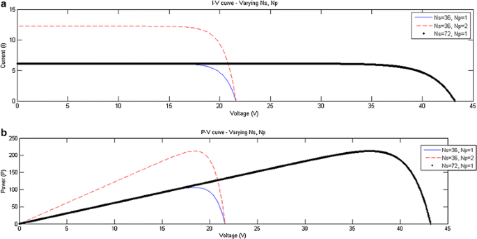
a I–V curve with varying Ns and Np. b P–V curve with varying Ns and Np
Summary
-
With two modules connected in series (Ns = 72, Np = 1), the value of current output is similar to that of it in case of one module (Ns = 36, Np = 1) but the voltage output doubles so the power output doubles.
-
In term of two modules connected in parallel (Ns = 36, Np = 2), the value of voltage output is similar to that of it in case of one module (Ns = 36, Np = 1) but the current output doubles so the power output doubles. Similar value of power output is experienced in both cases of two modules despite different ways in module connection (parallel or series).
The proposed model has advantages not only in studying effect of physical parameters such as series resistance Rs, shunt resistance Rsh, etc. but also in investigating impact of environmental condition like varying temperature, solar irradiation and especially shading effect. In this study, the evaluation of shading effect on solar PV array’s operation is carried out through following cases. The simulation results are given in Fig. 15a and b.
Fig. 15 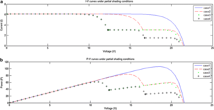
a I–V curves under partial shading condition. b P–V curves under partial shading condition
Case
Description
1
No shaded PV module (full irradiation on solar PV array): 1000 W/m2
2
One shaded module (receives irradiation of 500 W/m2), others receive full irradiation of 1000 W/m2
3
Two shaded modules (receive irradiation of 500 W/m2), others receive full irradiation of 1000 W/m2
4
Two shaded modules (receive irradiation of 500 and 250 W/m2), others receive irradiation of 1000 W/m2
Summary
-
The power output of PV array reduces noticeably when it works under partial shading condition.
-
The I–V curve experiences multiple steps whereas the P–V curve gives many local peaks along with the maximum power point (the global peak). In addition, more shaded modules are higher number of power output peaks is shown.
-


Experimental results and validation
The Matlab/Simulink model is evaluated for the experimental test system (two DS-100M panels are connected in series). The results are shown in Fig. 16. On the other hand, the empirical results with a solar irradiation of 520 W/m2 and operating temperature of 40 °C are given in Fig. 17. The I–V and P–V simulation and experimental results show a good agreement in terms of short circuit current, open circuit voltage and maximum power output.

Solar Matlab/SIMULINK results

Solar system experimental results
Conclusion
A step-by-step procedure for simulating a PV array with Tag tools, with user-friendly icons and dialogs in Matlab/Simulink block libraries is shown. This modeling procedure serves as an aid to help people to closer understand of I–V and P–V operating curves of PV module. In addition, it can be considered as a robust tool to predict the behavior of any solar PV cells, modules and arrays under varying environmental conditions (temperature, irradiation and partially shading condition) and physical parameters (series resistance, shunt resistance, ideality factor and so on). This research is the first step to study a hybrid system where a PV power generation connecting to other renewable energy production sources like wind or biomass energy systems.
References
Banu I-V, Istrate M (2012) Modeling and simulation of photovoltaic arrays. World energy system conference, p 6
Gonzalez-Longatt FM (2005) Model of photovoltaic module in Matab. II CIBELEC 2005, vol 2005, p 5
Gow JA, Manning CD (1999) Development of a photovoltaic array model for use in power-electronics simulation studies. IEEE Proc Electr Power Appl 146(2):8
Ibbini MS et al (2014) Simscape solar cells model analysis and design. In: Zaharim A, Sopian K, Bulucea A, Niola V, Skala V (eds) 8th International conference on renewable energy sources (RES’ 14), 2nd International conference on environmental informatics (ENINF’14), Kuala Lumpur, Malaysia, 23–25 April 2014, WSEAS Press
Jena C, Das A, Paniigrahi CK, Basu M (2014) Modelling and simulation of photovoltaic module with buck-boost converter. Int J Adv Eng Nano Technol 1(3):4
Mohammed SS (2011) Modeling and simulation of photovoltaic module using Matlab/Simulink. Int J Chem Environ Eng 2(5):6
Pandiarajan N, Muthu R (2011) Mathematical modeling of photovoltaic module with Simulink. International Conference on Electrical Energy Systems (ICEES 2011), p 6
Panwar S, Saini RP (2012) Development and simulation photovoltaic model using Matlab/Simulink and its parameter extraction. International conference on computing and control engineering (ICCCE 2012)
Salmi T, Bouzguenda M, Gastli A, Masmoudi A (2012) Matlab/simulink based modelling of solar photovoltaic cell. Int J Renew Energy Res 2(2):6
Savita Nema RKN, Agnihotri Gayatri (2010) Matlab/Simulink based study of photovoltaic cells/modules/arrays and their experimental verification. Int J Energy Environ 1(3):14
Sudeepika P, Khan GMG (2014) Analysis of mathematical model of PV cell module in Matlab/Simulink environment. Int J Adv Res Electr Electr Instrum Eng 3(3):7
Tu H-LT, Su Y-J (2008) Development of generalized photovoltaic model using MATLAB/SIMULINK. Proc World Congr Eng Comput Sci 2008:6
Varshney A, Tariq A (2014) Simulink model of solar array for photovoltaic power generation system. Int J Electr Electr Eng 7(2):8
Venkateswarlu G, Raju PS (2013) Simscape model of photovoltaic cell. Int J Adv Res Electr Electr Instrum Eng 2(5):7
Walker G (2001) Evaluating MPPT converter topologies using a Matlab PV model. J Electr Electr Eng Aust 21(1):7
Authors’ contributions
XHN initiated, proposed model developed in Matlab/Simulink and analyzed. He also prepared a draft manuscript for publication. MPN assisted in designing, data collection, analysis and reviewed the manuscript and edited many times and added his inputs. Finally, XHN decided finally the content of the research revised final manuscript. All authors read and approved the final manuscript.
Authors’ information
Xuan Hieu Nguyen is a lecturer in Department of Electric Power System, Faculty of Engineering, Vietnam National University of Agriculture, Hanoi, Vietnam. He had bachelor degree in electric power system, Hanoi University of Science and Technology, Vietnam in 2008. He received master degree in electrical engineering in University of Wollongong, Australia in 2012. Minh Phuong Nguyen is graduate student in Faculty of Engineering, Vietnam National University of Agriculture.
Acknowledgements
The authors are grateful to the support by this work through the project “Study, design and manufacture a solar PV system using SPV technology served for chicken farms in Faculty of Animal Science, Vietnam National University of Agriculture”, Vietnam (2014–2017).
Competing interests
The authors declare that they have no competing interests.
Author information
Authors and Affiliations
Corresponding author
Rights and permissions
Open Access This article is distributed under the terms of the Creative Commons Attribution 4.0 International License (http://creativecommons.org/licenses/by/4.0/), which permits unrestricted use, distribution, and reproduction in any medium, provided you give appropriate credit to the original author(s) and the source, provide a link to the Creative Commons license, and indicate if changes were made.
About this article

Cite this article
Nguyen, X.H., Nguyen, M.P. Mathematical modeling of photovoltaic cell/module/arrays with tags in Matlab/Simulink. Environ Syst Res 4, 24 (2015). https://doi.org/10.1186/s40068-015-0047-9
Received:
Accepted:
Published:
DOI: https://doi.org/10.1186/s40068-015-0047-9