International Trade

Abstract

Edgeworth (1894) opened his survey of the theory of international values with the provocative statement: ‘International trade meaning in plain English trade between nations, it is not surprising that the term should mean something else in Political Economy’. This could equally well be said today. What distinguishes international from domestic trade is the greater prevalence of barriers (both natural and artificial) to trade and factor movements in the former; different currencies; and (perhaps most important) autonomous governments, leading to a pattern of shocks which impact different countries in different ways. Because of these differences, a different type of theoretical model is called for. For example, international immobility of factors results in greater disparity in relative factor endowments among countries than among regions of the same country; these disparities may make it reasonable, as a first approximation, to ignore variations in supplies of factor services that come about in response to changes in factor rentals and commodity prices, if these variations are small in comparison with the differences in endowments. Likewise, great differences among resource endowments and productive techniques may make it reasonable to disregard differences in consumers’ tastes within and across countries, even though this might be a very inappropriate type of simplification for purposes of analysing domestic trade.

Edgeworth (1894) opened his survey of the theory of international values with the provocative statement: ‘International trade meaning in plain English trade between nations, it is not surprising that the term should mean something else in Political Economy’. This could equally well be said today. What distinguishes international from domestic trade is the greater prevalence of barriers (both natural and artificial) to trade and factor movements in the former; different currencies; and (perhaps most important) autonomous governments, leading to a pattern of shocks which impact different countries in different ways. Because of these differences, a different type of theoretical model is called for. For example, international immobility of factors results in greater disparity in relative factor endowments among countries than among regions of the same country; these disparities may make it reasonable, as a first approximation, to ignore variations in supplies of factor services that come about in response to changes in factor rentals and commodity prices, if these variations are small in comparison with the differences in endowments. Likewise, great differences among resource endowments and productive techniques may make it reasonable to disregard differences in consumers’ tastes within and across countries, even though this might be a very inappropriate type of simplification for purposes of analysing domestic trade.

The fact that national governments act independently leads to the need to analyse the effects of country-specific shocks, which take the form of intensification or liberalization of restrictions on trade or capital movements, unilateral transfers such as reparation payments, gifts, or loans, and disparities in monetary and fiscal policies. For this reason the emphasis in international-trade theory has from the beginning (Mill 1848; Marshall 1879) been on comparative statics: one wants to ascertain the qualitative, if not the quantitative, effect of a tariff or quota or transfer on the various quantities involved. To obtain unambiguous qualitative results one needs fairly drastic simplifications and strong assumptions. On the other hand, the emphasis in general-equilibrium theory (Walras 1874; Pareto 1896–97; Debreu 1959) has been on proving the existence, stability, and Pareto-optimality of competitive equilibrium, for which much milder assumptions are required. A good definition of international-trade theory as it has evolved would therefore be: ‘general-equilibrium theory with structure’.

The requirements of ‘simplicity’ in a theory are not absolute, but vary with the goals of the theory and the technical resources available to researchers at the time. There is not much virtue in simplicity if a result that holds in a model of two countries, two commodities, and two factors does not generalize in any meaningful way to higher dimensions. With the increasing possibilities of handling large-scale models and data sets and estimating their parameters numerically, it is natural to expect a movement of both general-equilibrium traditions towards each other.

Attention will be focused here on the neoclassical model developed by Haberler (1930, 1933), Lerner (1932, 1933, 1934), Ohlin (1928, 1933), Stolper and Samuelson (1941), Samuelson (1953), and Rybczynski (1955), which Baldwin (1982) has described as the ‘Haberler–Lerner–Samuelson model’ – an appellation which is more accurate than the usual ‘Heckscher–Ohlin theory’, since the model commonly employed makes the simplifying assumption – rejected by Ohlin (1933, ch. VII) except in his illustrative Appendix I – that factors of production are inelastic in supply and indifferent among alternative occupations, allowing one to define unambiguously a country’s production-possibility frontier. This model has in recent years come to lose some of its hold on the profession – just as the Ricardian theory had in the 1930s – in favour of models that stress imperfect competition (see, e.g. Helpman and Krugman 1985). However, these latter models have so far not been successfully formulated as general-equilibrium models, and are thus still in a formative stage. It goes without saying that, in the nature of the case, a partial-equilibrium model is incapable of explaining or predicting trade patterns or analysing the effect on prices and resource allocation of trade restrictions and transfers.

The material that follows is divided into two parts. Part 1 covers the mathematical foundations of the received theory, and deals with the duality between production functions and cost functions, the concept of a national-product function, the Stolper–Samuelson and Rybczynski relations between factor rentals and commodity prices and between commodity outputs and factor endowments, the concepts of trade-demand functions and trade-utility functions, world equilibrium and its dynamic stability. Part 2 covers the applications of these basic concepts to the most noteworthy problems that have been the object of attention in the theory of international trade since its beginnings: the explanation of trade flows, the effect of unilateral transfers on sectoral prices and resource allocation, and the effect of trade restrictions such as tariffs and quotas. The reader who is interested in substantive questions is advised to proceed directly to Part 2.

Part 1. The Mathematical Foundations

Duality of Cost Functions and Production Functions

Let an industry produce a positive amount y of output of a particular product, with the aid of non-negative amounts υ_j of m primary factors of production, determining the vector υ = (υ₁, υ₂,…, υ_m). A production function f is defined over the non-negative orthant ${E}_m^{+}$ of m-dimensional Euclidean space, with values y = f(υ) on the non-negative real line ${E}_1^{+}$. We assume that f has the following properties:

• (a) Upper semi-continuity: for each y the set

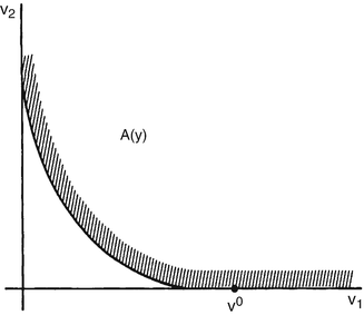
  $$ A(y)=\left\{\upsilon :f\left(\upsilon \right)>\right\} $$

  (1)

  is closed;

• (b) Quasi-concavity: for each y, the set A(y) defined by (1) is convex;

• (c) Monotonicity: if υ,υ´∈ ${E}_m^{+}$ are such that υ' ≧ υ, then f(υ') ≧ f(υ).

Further properties of f will be specified later on.

We shall denote by w = (w₁, w₂, …, w_m) a vector of factor rentals, i.e. prices of the services of the m factors of production. The following conventional notation will be adhered to:

$$ {\displaystyle \begin{array}{l}w\geqq 0\ \mathrm{means}\ {\mathrm{w}}_{\mathrm{i}}\geqq 0\ \mathrm{for}\ \mathrm{all}\ i=1,2,\dots, m;\\ {}w\geqq 0\ \mathrm{means}\ {\mathrm{w}}_{\mathrm{i}}\geqq 0\ \mathrm{for}\ \mathrm{all}\ i=1,2,\dots, m;\\ {}\kern4.56em and\ {w}_i>0\ \mathrm{for}\ \mathrm{some}\ i;\end{array}} $$

For each y > 0 and all w ≥ 0 we define the minimum total cost function G by

$$ G\left(w,y\right)=\underset{\upsilon }{\min}\left\{w\cdot \upsilon :f\left(\upsilon \right)\geqq y\right\}, $$

(2)

where w · υ denotes the inner product

$$ \sum_{j=1}^m{w}_j{\upsilon}_j $$

Mathematically, for each fixed y the function G(·, y) is the support function of the convex set A(y) (cf. Fenchel 1953). It has the following properties:

• (a*) Continuity in w: for each y, G(w, y) is continuous;

• (b*) Concavity in w: if 0 < θ < 1 then

  $$ \left(1-\theta \right)G\left({w}^o,y\right)+\theta G\left({W}^1,y\right)\leqq G\left[\left(1-\theta \right){w}^o+\theta {w}^1,y\right]; $$

• (c*) Monotonicity: y' ≧ y implies G(w, y') ≧ G(w, y) and w' ≧ w ≥ 0 implies G(w', y) ≧ G(w, y);

• (d*) positive homogeneity in w : G(λw, y) = λG(w, y) for all λ > 0.

Property (a*) follows from (a) and the definition of G; property (c*) follows the definition of G and the fact that y' ≧ y implies A(y') ⊆ A(y); property (d*) follows immediately from the definition of G. To prove (b*), let w⁰, w¹ ≥ 0 and denote w^θ = (1–θ)w⁰ + θw¹; from the definitions of G and A(y) in (2) and (1), we have

$$ {\displaystyle \begin{array}{l}G\left({w}^o,y\right)\leqq {w}^o\cdot \upsilon\ \mathrm{for}\ \mathrm{all}\ v\in A(y);\\ {}G\left({w}^1,y\right)\leqq {w}^1\cdot y\ \mathrm{for}\ \mathrm{all}\ v\in A(y);\end{array}} $$

consequently,

$$ \left(1-\theta \right)G\left({w}^o,y\right)+\theta G\left({W}^1,y\right)\leqq {w}^o\cdot v\ \mathrm{for}\ \mathrm{all}\ v\in A(y). $$

Hence, in particular,

$$ \left(1-\theta \right)G\left({w}^o,y\right)+\theta G\left({w}^1\cdot y\right)\leqq \min \left\{{w}^{\theta}\cdot \upsilon :\upsilon \in A(y)\right\}\equiv G\left({W}^{\theta },y\right), $$

which is the result sought (cf. Uzawa 1964b).

Of fundamental importance in international trade theory is the following duality theorem first proved by Shephard (1953). The formulation and proof contained in Theorem 1 to follow are due to Uzawa (1964b).

Theorem 1

(Duality Theorem). Define the set

$$ B(y)=\left\{\upsilon :\left(\forall w\ge 0\right)w\cdot \upsilon \geqq G\left(w,y\right)\right\}, $$

(3)

where G is defined by (2) and f satisfies properties (a), (b), (c). Then B(y) = A(y), where A(y) is defined by (1).

Proof:

Let υ⁰ ∈ A(y); then f(υ⁰) ≧ y, so for all w ≥ 0,

$$ w\cdot {\upsilon}^o\geqq \underset{\upsilon }{\min}\left\{w{\cdot}^u:f\left(\upsilon \right)\geqq y\right\}\equiv G\left(w,y\right) $$

that is, υ⁰ ∈ B(y).

Conversely, suppose υ⁰$\notin$A(y). Since A(y) is closed and convex by properties (a) and (b) of f, it follows from the separating hyperplane theorem of closed convex sets (cf. Fenchel 1953, p. 48) that there exists a vector w⁰ ≠ 0 such that

$$ {w}^0\cdotp {\upsilon}^0<\underset{\upsilon }{\min}\left\{{w}^0.\upsilon :\upsilon \in A(y)\right\} $$

(4)

(see Fig. 1). Now if w⁰ has a negative component, it follows from property (c) that the corresponding component of υ ∈ A(y) may be chosen to be arbitrarily large, hence no minimum of w⁰ · v over A(y) exists; consequently, w ≥ 0. But then the expression on the right of the inequality sign in (4) is just G(w⁰, y). From the definition of B(y) in (3), it follows that υ⁰$\notin$

International Trade, Fig. 1

B(y). q.e.d.

The duality theorem may be stated in words as follows: given the function G, the set A(y) may be identified with the set of all factor combinations υ which, at each constellation w ≥ 0 of factor rentals, are at least as expensive as the minimal total cost of producing output y at factor rentals w.

Let us now explore the consequences of imposing a further condition on the production function f:

• (d) Positive homogeneity: for all λ > 0, f(λυ) = λf(υ).

From the definition of G in (2), we now have

$$ {\displaystyle \begin{array}{c}G\left(w,y\right)=\underset{\upsilon }{\min \limits}\left\{w\cdot \upsilon :f\left(\frac{\upsilon }{y}\right)\geqq 1\right\}\\ {}=\underset{b}{\min \limits}\left\{ yw\cdot b:f(b)\geqq 1\right\}\left(b=\frac{u}{y}\right)\\ {}=y\cdot \underset{b}{\min \limits}\left\{w\cdot b:f(b)\geqq 1\right\}.\end{array}} $$

Thus, G(w, y) factors into two terms, of which the second depends only on w ≥ 0 and may be denoted

$$ g(w)=\underset{\upsilon }{\min}\left\{w\cdot \upsilon :f\left(\upsilon \right)\geqq 1\right\}. $$

(5)

We therefore have

Theorem 2.

If f satisfies properties (a), (b), (c), (d), then the function G of (3) factors into

$$ G\left(w,y\right)= yg(w) $$

(6)

where g is defined by (5) and is continuous, concave, monotone, and positively homogeneous of first degree.

The properties of g specified in Theorem 2 follow directly from those of the function G.

We may now state a special form of the duality theorem for the case of homogeneous production functions.

Theorem 3.

Let g be defined by (5) where f satisfies properties (a), (b), (c), (d), and let the function f* be defined by

$$ {f}^{\ast}\left(\upsilon \right)=\underset{\upsilon }{\min}\left\{w\cdot \upsilon :g(w)\geqq 1\right\}. $$

(7)

Then f * = f.

Proof:

Define the set

$$ C(y)=\left\{\upsilon :\left[\forall w\in {A}^{\ast }(1)\right]w\cdot \upsilon \geqq y\right\} $$

(8)

where for convenience we define

$$ {A}^{\ast }(p)=\left\{w:g(w)\geqq p\right\}. $$

(9)

(Since g is defined only for w ≥ 0, w ∈ A*(p) implies w ≥ 0). First we shall show that C(y) = B(y), where B(y) is defined by (3). From (3) and (6), if υ⁰ ∈ B(y) then for all w ∈ A*(1), w · v⁰ ≧ G(w, y) = yg(w) ≥ y, so B(y) ⊆ C(y). Conversely suppose v⁰ ∈ C(y) and take any w⁰ ≥ 0. Then from the homogeneity of g we have g[w⁰/g(w⁰)] = 1, hence from the definition (8) of C(y) it follows that

$$ \frac{w^o}{g\left({w}^o\right)}\cdot {\upsilon}^o\geqq y, $$

i.e., w⁰ · v⁰ ≧ yg(w⁰); thus v⁰ ∈ B(y). Therefore B(y) = C(y) and by Theorem 1, C(y) = A(y).

Now denote r = w/g(w) and consider the set

$$ {C}^{\prime }(y)=\left[\upsilon :\underset{r}{\min}\left\{r\cdot \upsilon :r\in {A}^{\ast }(1)\right\}\geqq y\right]. $$

(10)

If r · v ≧ y for all r ∈ A*(1), then a fortiori r · v ·≧ y for the r ∈ A*(1) which minimizes r · v; hence C(y) ⊆ C′(y). Conversely, for all r ∈ A*(1) we have r · υ ≧ min_r {r · υ : r ∈ A*(1)}, so C′(y) ⊆ C(y). Thus C′(y) = C(y) = A(y). But from (7), (9) and (10) we have

$$ {C}^{\prime }(y)=\left\{\upsilon :{f}^{\ast}\left(\upsilon \right)\geqq y\right\}. $$

(11)

Since A(y) = C′(y) for all y, therefore f and f * coincide.

q.e.d.

Let us consider the consequences of adding to the properties (a), (b), (c) of f given in §1.1 the following further properties:

• (b₁) Strict quasi-concavity: for each y, the set A(y) defined by (1) is strictly convex;

• (e) Differentiability: f has continuous first-order partial derivatives (Fig. 2).

  

  International Trade, Fig. 2

For the time being, property (d) of §1.2 will not be used, but will be introduced again later on.

The problem of deriving the minimum total cost function G(w, y) may be posed in terms of the following non-linear programming problem:

$$ \mathrm{minimize}\;\sum_{j=I}^m{w}_j{\upsilon}_j\ \mathrm{subject}\ \mathrm{to}\ f\left(\upsilon \right)\geqq y,u\geqq 0 $$

(12)

Form the Lagrangean function

$$ L\left({p}^{\ast },u;y,w\right)=\sum_{j=I}^m{w}_j{\upsilon}_j-{p}^{\ast}\left[f\left(\upsilon \right)-y\right] $$

(13)

where y, w are parameters and p* is a Lagrangean multiplier. In accordance with the Kuhn–Tucker theorem (cf. Kuhn and Tucker 1951, p. 486) in order for ${\upsilon}^0=\left({\upsilon}_1^0,{\upsilon}_2^0,\dots, {\upsilon}_m^0\right)$ to be a solution of the minimum problem (12), it is necessary and sufficient that υ⁰ and some p* ≧ 0 satisfy

$$ {\left.\frac{\partial L}{\partial {\upsilon}_j}\right|}_{\upsilon ={\upsilon}^0}= wj-{p}^{\ast }{\left.\frac{\partial f}{\partial {v}_j}\right|}_{\upsilon ={\upsilon}^0}\geqq 0: uj\frac{\partial L}{\partial {\upsilon}_j}=0 $$

(14)

and

$$ \sum_{j=1}^m{\upsilon}_j^0{\left.\frac{\partial L}{\partial {\upsilon}_j}\right|}_{\upsilon j={\upsilon}_j^0}=\sum_{j=1}^m{\upsilon}_j^0\left({w}_j-{p}^{\ast }{\left.\frac{\partial L}{\partial {\upsilon}_j}\right|}_{\upsilon j={\upsilon}_j^0}\right)=0 $$

(15)

as well as

$$ \frac{\partial L}{\partial {p}^{\ast }}=-\left[f\left({\upsilon}^0\right)-y\right]\geqq 0;{p}^{\ast}\frac{\partial L}{\partial {p}^{\ast }}=0. $$

(16)

In the above we have used (e), but so far property (b₁) has not yet been used: Let us introduce the further properties:

• (f) indispensability: f(0) = 0.

• (f₁) strict indispensability: if υ has a component υ_j = 0 then f(υ) = 0.

Now suppose the solution υ⁰ to (12) is such that f(υ)⁰ > y (see Fig. 2). This violates (b₁), since strict quasi-concavity requires that if υ⁰, υ¹ ∈ A(y) and 0 < θ < 1, the point υ⁰ = (1 – θ)v⁰ + θυ¹ should be in the interior of A(y). Suppose, however, that property (b₁) is not assumed, and that f(υ⁰) > y > 0; then p* = 0 from (16) hence w · υ⁰ = 0 from (15), and since w ≥ 0 this implies that υ⁰ has a zero component. Thus, if (f₁) is assumed, we have 0 = f(υ⁰) > y > 0 – a contradiction. Thus, either (b₁) or (f₁) is sufficient – in conjunction with (a), (c), (e), to guarantee f(υ⁰) = y. If w > 0, a similar argument shows that (f) implies f(υ⁰) = y.

Now suppose that υ⁰ is such that strict inequality holds in (14) for some j. Then υ⁰_j = 0 from (15) If (f₁) holds this would lead to a contradiction, since then 0 = f(υ⁰)≧ y > 0. If (f₁) is not assumed, but if (b₁) holds, then strict inequality in (14) implies that υ⁰ has a zero component, so υ⁰ is on the boundary of A(y); but 2υ⁰ is also on the boundary of A(y), by property (c), and consequently the mid-point $1\frac{1}{2}{\upsilon}^0$ is as well, contradicting (b₁). Thus, if (a), (b), (c), (e) hold, then either (b₁) or (f₁) implies that equality holds in (14) for all j = 1, 2,…, m.

Consider a solution υ⁰ to (12) corresponding to a w⁰ which has some zero components. Let J = {j: w⁰_j = 0}. Then if w⁰ · υ⁰ = C⁰, certainly A(y) ⊆ {υ: w⁰ · υ⁰ ≧ C⁰}. Let υ¹ be such that υ¹_j > υ⁰_j for j ∈ J and υ¹_j = υ⁰_j for j$\notin$J. Then w⁰ · υ¹ = w⁰ · υ⁰, hence υ¹ ∈ {υ: w⁰ · υ = C⁰}. But by condition (c), υ¹ ∈ A(y); thus υ¹ and υ⁰ are both on the boundary of A(y), as is (1 –θ)υ⁰ + θυ¹ for 0 < θ < 1 (see Fig. 3). This contradicts (b₁). Therefore under (b₁), a solution to (12) exists only if w > 0.

International Trade, Fig. 3

It should be noted that even if the function G(w, y) of (2) is well defined in the sense

$$ G\left(w,y\right)=\underset{v}{\inf}\left\{w\cdot \upsilon :f\left(\upsilon \right)\geqq y\right\}, $$

(17)

a solution of (12) need not exist. For example, if

$$ f\left({\upsilon}_1,{\upsilon}_2\right)=\frac{1}{\frac{1}{\upsilon_1}+\frac{1}{\upsilon_2}} $$

Then

$$ G\left(0,{w}_2;y\right)=y{w}_2 $$

but the infimum is achieved as (υ₁, υ₂) → (∞, y). On the other hand a solution to (12) always exists if w > 0; for, choosing any υ⁰ ∈ int A(y) and w⁰ > 0, the set

$$ A(y)\cap \left\{\upsilon :{w}^0\cdot \upsilon \leqq {w}^0{\upsilon}^0,\upsilon \geqq 0\right\} $$

is compact by virtue of condition (a), and from (b) and (c) the minimum of w⁰· υ over this set is the minimum over A(y).

An immediate consequence of (b₁) is that if (12) has a solution, it is unique. Since (12) need not have a solution unless w > 0, it is of some advantage to replace (b₁) by a weaker condition which still ensures uniqueness provided w > 0. Such a condition is

(b₂) if υ⁰ ≠ υ¹ and neither υ⁰ ≥ υ¹ nor υ¹ ≥ υ⁰, and if 0 < θ < 1, then f [(1 – θ)υ⁰ + θυ¹] > min[f(υ⁰), f(υ¹)].

The above discussion may now be summarized in the following theorem.

Theorem 4.

Let conditions (a), (b), (c), (e), (f) hold. Then if either (b₁) or (f₁) holds, any solution υ⁰ to (12) has the property (Fig. 3)

$$ {w}_j={p}^{\ast }{\left.\frac{\partial f}{\partial {\upsilon}_j}\right|}_{\upsilon ={\upsilon}^0}\left(j=1,2,\dots, m\right);f\left({\upsilon}^0\right)=y. $$

(18)

If (b₁) holds, this solution is unique. If (b₂) holds and if w > 0, then a unique solution to (12) exists, and it satisfies (18).

We now proceed with an analysis of the solution υ of the programming problem (12) regarded as a function of the parameters y > 0, w > 0, when conditions (a), (b₂), (c), (e), (f) are assumed to hold.

In accordance with Theorem 4, the solution satisfies (18) and is unique, given y and w. Thus we have the functions

$$ {\upsilon}_j=\upsilon \left(w,y\right)\kern2.25em \left(j=1,2,\dots, m\right). $$

(19)

It is shown in Fenchel (1953, pp. 102–4) that these functions are differentiable. Substituting (19) into (18) we obtain

$$ {p}^{\ast }={w}_j/\frac{\partial }{\partial {\upsilon}_j}f\Big[{\tilde{\upsilon}}_1\left(w,y\right),\kern1em {\tilde{\upsilon}}_2\left(w,y\right),\dots {\tilde{\upsilon}}_m\left(w,y\right)={\tilde{p}}^{\ast}\left(w,y\right). $$

The system of equations (18) defines a mapping $\mathrm{F}$ from the non-negative orthant of (m + 1)-dimensional space into itself:

$${\mathrm{F}}^{-1}\left(\upsilon ,p^{*}\right)=\left(w,y\right)\text{.}$$

(20)

Equations (19) and (1.13b) define the inverse mapping:

$${\mathrm{F}}^{-1}\left(w,y\right)=\left(\upsilon ,p^{*}\right)\text{.}$$

(21)

In accordance with (2) we define

$$ G\left(w,y\right)=\sum_{k=1}^m{w}_k{\tilde{\upsilon}}_k\left(w,y\right). $$

(22)

We shall also define the indirect production function f by

$$ \tilde{f}\left(w,y\right)=f\left[{\tilde{\upsilon}}_1\left(w,y\right),{\tilde{\upsilon}}_2\left(w,y\right)\right],\dots, {\tilde{\upsilon}}_m\left(w,y\right)\Big] $$

(23)

which satisfies the identity

$$ \tilde{f}\left(w,y\right)=y\ \mathrm{for}\ \mathrm{all}\ w,y. $$

(24)

Theorem 5.

(Fundamental Envelope Theorem of Production Theory). The functions G,${\tilde{\upsilon}}_l$, ${\tilde{p}}^{\ast }$ of (22), (19), (1.13b) are related by

$$ \frac{\partial G\left(w,y\right)}{\partial {w}_j}={\tilde{\upsilon}}_j\left(w,y\right)\kern1em j=1,2,\dots, m $$

(25)

and

$$ \frac{\partial G\left(w,y\right)}{\partial {w}_j}={\tilde{p}}^{\ast}\left(w,y\right) $$

(26)

Proof:

Differentiating (15) with respect to w_j, we obtain

$$ \frac{\partial G\left(w,y\right)}{\partial {w}_j}={\tilde{\upsilon}}_j\left(w,y\right)+\sum_{k=1}^m{w}_k\frac{\partial {\tilde{\upsilon}}_k\left(w,y\right)}{\partial {w}_j} $$

(27)

To prove (25) we must show that the second term on the right of (27) vanishes. Differentiating (23) with respect to w_j and making use of the identity (24) and the chain rule, we obtain upon substitution of (1.13b),

$$ 0=\frac{\partial f\left(w,y\right)}{\partial {w}_j}=\sum_{k=1}^m{\left.\frac{\partial f}{\partial {\upsilon}_k}\right|}_{\upsilon k=\tilde{\upsilon}k\left(w,y\right)}\cdot \frac{\partial {\tilde{\upsilon}}_k\left(w,y\right)}{\partial {w}_j}=\frac{1}{{\tilde{p}}^{\ast}\left(w,y\right)}\sum_{k=1}^m{w}_k\frac{\partial {\tilde{\upsilon}}_k\left(w,y\right)}{\partial {w}_j}. $$

and (25) follows. Likewise, differentiating (23) with respect to y and using the identity (24) and the chain rule, we have upon making use once again of (1.13b),

$$ 1=\frac{\partial \tilde{f}\left(w,y\right)}{\partial y}=\sum_{k=1}^m{\left(\frac{\partial f}{\partial {\upsilon}_k}\right)}_{\upsilon k=\tilde{\upsilon}k\left(w,y\right)}\cdot \frac{\partial {\tilde{\upsilon}}_k\left(w,y\right)}{\partial y}=\frac{1}{{\tilde{p}}^{\ast}\left(w,y\right)}\sum_{k=1}^m{w}_k\frac{\partial {\tilde{\upsilon}}_k\left(w,y\right)}{\partial y}. $$

Thus, from this result and (22),

$$ \frac{\partial G\left(w,y\right)}{\partial y}=\sum_{k=1}^m{w}_k\frac{\partial {\tilde{\upsilon}}_k\left(w,y\right)}{\partial y}={\tilde{p}}^{\ast}\left(w,y\right), $$

establishing (26).

q.e.d.

It may be noted immediately from (22) and (25) that

$$ G\left(w,y\right)=\sum_{k=1}^m{w}_k\frac{\partial G\left(w,y\right)}{\partial {w}_k}, $$

providing the necessary and sufficient condition, by Euler’s theorem, that G be homogeneous of degree 1 in w – a result already obtained in §1.1. Using (25) again it follows that ${\tilde{\upsilon}}_j$ is homogeneous of degree zero in w.

Now let us introduce condition (d): the positive homogeneity (of degree 1) of the production function f. Using (22) and (1.13b) we have, by Euler’s theorem,

$$ {\displaystyle \begin{array}{c}G\left(w,y\right)=\sum \limits_{k=1}^m{w}_k{\tilde{\upsilon}}_k\left(w,y\right)\\ {}={\tilde{p}}^{\ast}\left(w,y\right)\sum \limits_{k=1}^m{\left(\frac{\partial f}{\partial {\upsilon}_k}\right)}_{\upsilon k=\tilde{\upsilon}k\left(w,y\right)}\cdot {\tilde{\upsilon}}_k\left(w,y\right)\\ {}=y{\tilde{p}}^{\ast}\left(w,y\right)\end{array}} $$

whence from (6)

$$ {\tilde{p}}^{\ast}\left(w,y\right)=\frac{G\left(w,y\right)}{y}=g(w). $$

(28)

Defining

$$ {b}_j(w)=\frac{\partial g(w)}{\partial {w}_j}\kern1em \left(j=1,2,\dots, m\right) $$

(29)

we have from (25), (28), and (29),

$$ {\tilde{\upsilon}}_j\left(w,y\right)=\frac{\partial G\left(w,y\right)}{\partial {w}_j}=y\frac{\partial g(w)}{\partial {w}_j}=y{b}_j(w) $$

(30)

hence the optimal factor-product ratios are given by

$$ \frac{\upsilon_j}{y}={b}_j(w). $$

(31)

From the differentiability assumption (e) imposed on the function f we can derive a strict quasi-concavity property of the function g. For suppose w⁰ > 0, w¹ > 0, and w⁰ ≠ λw¹; then from (b₂) and (e), we have b(w⁰) ≠ b(w¹), where

$$ b(w)=\left[{b}_1(w),{b}_2(w),\dots, {b}_a(w)\right]. $$

(32)

Now by definition of g [see (5)]

$$ {\displaystyle \begin{array}{l}g\left({w}^0\right)\leqq {w}^0\cdot \upsilon\ \mathrm{for}\ \mathrm{all}\ \upsilon \in A(1)\\ {}g\left({w}^1\right)\geqq {w}^1\cdot \upsilon\ \mathrm{for}\ \mathrm{all}\ \upsilon \in A(1)\end{array}} $$

(33)

and moreover

$$ {\displaystyle \begin{array}{l}g\left({w}^0\right)={w}^0\cdot \upsilon\ \mathrm{if}\ \mathrm{and}\ \mathrm{only}\ \mathrm{if}\ \upsilon \in b\left({w}^0\right)\\ {}g\left({w}^1\right)\geqq {w}^1\cdot \upsilon\ \mathrm{if}\ \mathrm{and}\ \mathrm{only}\ \mathrm{if}\ \upsilon \in b\left({w}^0\right)\end{array}} $$

(34)

Furthermore, b(w⁰) ≠ b(w¹), so strict inequality must hold in one of the inequalities (33); thus if 0 < θ < 1,

$$ \left(1-\uptheta \right)g\left({w}^0\right)+\uptheta g\left({w}^1\right)<\left[\left(1-\uptheta \right){w}^0+\uptheta {w}^1\right]\cdot v\ \mathrm{for}\ \mathrm{all}\ v\in A(1) $$

and therefore in particular

$$ {\displaystyle \begin{array}{l}\left(1-\theta \right)g\left({w}^0\right)+\theta g\left({w}^1\right)\\ {}<\underset{v}{\min \limits}\left\{\left[\left(1-\theta \right){w}^0+\theta {w}^1\right]\cdot v:v\in A(1)\right\}\\ {}=g\left[\left(1-\theta \right){w}^0+\theta {w}^1\right].\end{array}} $$

So we have

(b*) if w⁰ > 0, w¹ > 0, and w⁰ ≠ λw¹, and if 0 < θ < 1, then g[(1 – θ)w⁰ + θw¹] > (1 – θ)g(w⁰) + θg(w¹).

If is not hard to see that a corresponding property (b₃) holds for f as well. Failure of $\left({b}_3^{\ast}\right)$ when f is not differentiable, allowing b(w⁰) = b(w¹) for w⁰ ≠ λw¹, is illustrated in Fig. 4.

International Trade, Fig. 4

In general, a flat segment on a production isoquant goes over into a kink on the dual cost isoquant, and vice versa. There is another still more subtle relationship, illustrated by the following function found in Katzner (1970, p. 54):

$$ f\left({\upsilon}_1,{\upsilon}_2\right)={\left({\upsilon}_1^3{\upsilon}_2+{\upsilon}_1{\upsilon}_2^3\right)}^{1/4} $$

Its dual minimum-unit-cost function is found to be

$$ g\left({w}_1,{w}_2\right)={2}^{-1/4}{\left[{\left({w}_1+{w}_2\right)}^{4/3}-{\left({w}_1\ {w}_2\right)}^{4/3}\right]}^{4/3}. $$

The isoquants of f are extremely flat at υ₁ = υ₂, and as a result g is once but not twice differentiable at w₁ = w₂. A graph of

$$ g\left({w}_1,{w}_2\right)={w}_1{b}_1\left({w}_1,{w}_2\right)+{w}_2{b}_2\left({w}_1\ {w}_2\right) $$

for ${w}_2={\overline{w}}_2$ is shown in Fig. 5. At ${w}_1={\overline{w}}_2,{\overline{w}}_2{b}_2\left({w}_1,{\overline{w}}_2\right)$ has a slope of +∞ and ${w}_1{b}_1\left({w}_1,{\overline{w}}_2\right)$ has a slope of –∞, yet their sum is differentiable. When the bordered Hessian of the production function f is invertible, its inverse is the bordered Hessian of the cost function g; in the above example, it is not invertible at υ₁ = υ₂.

International Trade, Fig. 5

A useful illustration of the duality of cost and production functions is given by the case of CES (constant-elasticity-of-substitution) production functions (cf. Arrow et al. 1961; Uzawa 1962):

$$ f\left(\upsilon \right)={\left[\sum_{i=1}^m{\alpha}_i{\upsilon}_i^{1-1/\sigma}\right]}^{\sigma /\left(\sigma -1\right)} $$

The corresponding cost functions have the form

$$ f(w)={\left[\sum_{i=1}^m{\alpha}_i^{\sigma }{w}_i^{1-\sigma}\right]}^{1/\left(1-\sigma \right)} $$

whose elasticity of substitution is σ* = 1/σ.

The Production-Possibility Set

Suppose a country to be capable of producing n commodities with the aid of m primary factors of production. Denoting the output of commodity j by y_j, and the input of factor i into the production of commodity j by υ_ij, the production function may be written

$$ {y}_j={f}_i\left({\upsilon}_{1j},{\upsilon}_{2j},\dots, {v}_{mj}\right)={f}_j\left({\upsilon}_j\right)\kern1.5em \left(j=1,2,\dots, n\right), $$

(35)

where

$$ {\upsilon}_{.j}=\left({\upsilon}_{1j},{\upsilon}_{2j},\dots, {\upsilon}_{mj}\right). $$

(36)

It will be assumed that f_j is:

• (a) Continuous; i.e.,

  $$ \underset{\upsilon_j\to {\upsilon}_j^0}{\lim}\;{f}_j\left({\upsilon}_j\right)={f}_j\left({\upsilon}_j^0\right); $$

• (b) Weakly monotone; i.e., if ${\upsilon^1}_{.j}\geqq {\upsilon^2}_{.j}$ (meaning that ${\upsilon^1}_{ij}\geqq {\upsilon^2}_{ij}$ for i = 1, 2,…,m) then ${f}_i\left({\upsilon^1}_{.j}\right)\geqq {f}_j\left({\upsilon^2}_{.j}\right)$, and if ${\upsilon^1}_{.j}>{\upsilon^2}_{.j}$ (i.e., ${\upsilon^1}_{ij}>{\upsilon^2}_{ij}$ for i = 1, 2,…, m) then ${f}_i\left({\upsilon^1}_{.j}\right)>{f}_j\left({\upsilon^2}_{.j}\right);$

• (c) Concave; i.e., if υ⁰_{. j} and υ¹_{. j} are any two vectors of primary inputs into the production of commodity j, then for any t in the interval 0 < t < 1, (Fig. 5)

  $$ {f}_j\Big[\left(1-t\right){\upsilon}_j^0+t{\upsilon}_j^1\geqq \left(1-t\right){f}_j\left({\upsilon}_j^0\right)+t{f}_j\left({\upsilon}_j^1\right) $$

  (37)

• (d) Positively homogeneous of degree 1; i.e., for any λ > 0,

  $$ {f}_j\left(\lambda {\upsilon}_{.j}\right)=\lambda {f}_j\left({\upsilon}_{.j}\right). $$

  (38)

It will be convenient to introduce the m × n allocation matrix

$$ V=\left[\begin{array}{cccc}\hfill {\upsilon}_{11}\hfill & \hfill {\upsilon}_{12}\hfill & \hfill \cdots \hfill & \hfill {\upsilon}_{1n}\hfill \\ {}\hfill {\upsilon}_{21}\hfill & \hfill {\upsilon}_{22}\hfill & \hfill \cdots \hfill & \hfill {\upsilon}_{2n}\hfill \\ {}\hfill \cdot \hfill & \hfill \cdot \hfill & \hfill \cdot \hfill & \hfill \cdot \hfill \\ {}\hfill {\upsilon}_{m1}\hfill & \hfill {\upsilon}_{m2}\hfill & \hfill \cdots \hfill & \hfill {\upsilon}_{mn}\hfill \end{array}\right] $$

(39)

The element υ_ij is the input of factor i into the production of commodity j. The j the column of V will be donoted υ_j; according to this notation, υ_j is the transpose of υ_{. j}, denoted υ_j = v′_.j.

Let l_i denote the country’s total endowment of factor i. Then for each i the following resource constraint holds:

$$ \sum_{j=1}^m{\upsilon}_{ij}\leqq {l}_j\kern1em \left(i=1,2,\dots m\right). $$

(40)

Using (39) this can be written in matrix notation as

$$ \left[\begin{array}{cccc}\hfill {\upsilon}_{11}\hfill & \hfill {\upsilon}_{12}\hfill & \hfill \cdots \hfill & \hfill {\upsilon}_{1n}\hfill \\ {}\hfill {\upsilon}_{21}\hfill & \hfill {\upsilon}_{22}\hfill & \hfill \cdots \hfill & \hfill {\upsilon}_{2n}\hfill \\ {}\hfill \cdot \hfill & \hfill \cdot \hfill & \hfill \cdots \hfill & \hfill \cdot \hfill \\ {}\hfill {\upsilon}_{m1}\hfill & \hfill {\upsilon}_{m2}\hfill & \hfill \cdots \hfill & \hfill {\upsilon}_{mn}\hfill \end{array}\right]\left[\begin{array}{c}\hfill 1\hfill \\ {}\hfill 1\hfill \\ {}\hfill \vdots \hfill \\ {}\hfill 1\hfill \end{array}\right]\leqq \left[\begin{array}{c}\hfill {l}_1\hfill \\ {}\hfill {l}_2\hfill \\ {}\hfill \vdots \hfill \\ {}\hfill {l}_m\hfill \end{array}\right], $$

(41)

or simply

$$ {V}_i\leqq l, $$

(42)

where l is the column vector of n ones and l = (l₁, l₂,…,l_m)′ is the column vector of factor endowments.

In the absence of any additional restrictions, condition (40) expresses the perfectly mobility of factors among industries.

The country’s production–possibility set is the set of all possible output combinations y = (y₁, y₂,…,y_n) that can be produced with the production functions (35) under the resource constraints (40). Formally, it may be denoted

$$\begin{array}{l}\mathrm{Y}\left(l\right)\hfill \\ =y:\mathrm{there}\mathrm{exist}\mathrm{allocations}{\upsilon }_{ij}\geqq 0\mathit{such}\mathit{that}{y}_j=f_j\left({\upsilon }_j\right)\left(j=1,2,\dots n\right)\mathrm{and}{\displaystyle \sum _{j=1}^n{\upsilon }_{ij}}\leqq l_j\left(i=1,2,\dots m\right)\text{.}\hfill \end{array}$$

(43)

For notational convenience we may define the function f(V) as the vector-valued function

$$ f(V)={\left({f}_1\left({\upsilon}_1^{\hbox{'}}\right),{f}_2\left({\upsilon}_2^{\hbox{'}}\right),\dots, {f}_n\left({\upsilon}_n^{\hbox{'}}\right)\right)}^{\prime } $$

(44)

and write (43) in the more compact form

$$ y(l)=\left\{y:\left(\exists V\geqq 0\right)y=f(V)\&{V}_l\geqq l\right\}. $$

(45)

Note that with this notation, condition (37) can be written (for t = t_j) in the form

$$ f\left({V}^0\left(I-T\right)+{V}^1T\right)\geqq \left(I-T\right)f\left({V}^0\right)+ Tf\left({V}^1\right) $$

(46)

where T = diag(t₁, t₂,…,t_n) is an n × n diagonal matrix with 0 < t_j < 1. Likewise, (38) may be written (for λ = λ_j) in the form

$$ f\left( V\varLambda \right)=\varLambda f(V), $$

(47)

where Λ = diag(λ₁, λ₂,…,λ_n) is an n × n diagonal matrix with λ_j > 0.

Theorem 6.

If assumptions (a), (b), and (c) hold, the production-possibility set $\mathrm{Y}$(l) is convex.

Proof:

Let y⁰, y¹ both belong to $\mathrm{Y}$(l); we are to show that for any t in the interval 0 < t < 1, the output combination y^t = (l – t) y⁰ + ty¹ also belongs to $\mathcal{Y}$(l) (see Fig. 6).

International Trade, Fig. 6

Since y⁰, y^ty ∈ $\mathrm{Y}$(l), this means that there exist two allocation matrices V⁰, V¹ each satisfying (42), such that y⁰ = f(V⁰) and y¹ = f(V¹). Denote V^t = (1 –t)V⁰ + tV⁰. Then from (42),

$$ {V}^tl=\left(1-t\right){V}^0t+t{V}^1l\leqq \left(1-t\right)l+ tl=l, $$

(48)

so V^t is a feasible allocation, and by concavity,

$$ f\left({V}^t\right)\geqq \left(1-t\right)f\left({V}^0\right)+ tf\left({V}^1\right)={y}^t, $$

(49)

i.e., for each j = 1, 2,…, n, denoting ${\upsilon^t}_{.j}={{\left(1-t\right)}^{\mathrm{V}}}_{.j}+t{\upsilon^1}_{.j},$

$$ {f}_j\left({\upsilon^t}_{.j}\right)\geqq \left(1-t\right){f}_j\left({\upsilon^0}_{.j}\right)+t{f}_j\left({\upsilon^1}_{.j}\right)={y^t}_j. $$

(50)

By continuity and monotonicity of f_j, there exist ${\uplambda^t}_j\leqq 1$ such that

$$ {f}_j\left({\uplambda}_j^t{\upsilon}_j^t\right)={y}_j^t\kern1em \left(j=1,2,\dots, n\right). $$

(51)

(In particular, (51) follows if the stronger homogeneity condition (d) holds, by taking ${\lambda^t}_j={y}_j^t/{f}_j\left({\upsilon}_{.j}^t\right)$ if ${y^t}_t>0$, and 0 otherwise.) Equivalently,

$$ f\left({V}^t{\varLambda}^t\right)={y}^t. $$

(52)

It remains only to verify that the matrix V^tΛ of allocations λ^t_j υ^t_ij satisfies the constraint (42).

This is immediate from the fact that $0\leqq {\uplambda}_j^t\leqq \kern1em 1$, whence from (48),

$$ {V}^t{\varLambda}_l^t={V}^t{\lambda}^t\leqq {V}_l^t\leqq l. $$

(53)

q.e.d.

Note that homogeneity of production functions is not needed for the above result (Fig. 7).

International Trade, Fig. 7

The National-Product Function

Letp = (p₁, p₂,…, p_n)′ denote a vector of prices. Thenational-product function(cf. Samuelson 1953; Chipman 1972, 1974) is defined as the function

$$\Pi \left(p,l\right)=\underset{y{\in }_{\mathrm{Y}}\left(l\right)}{max}p\cdot y\text{.}$$

(54)

[See also Dixit and Norman (1980), who use the terminology ‘revenue function’.]

For any fixed p, this has all the properties of a production function, but with some special peculiar features. These are illustrated in Fig. 7 to be explained shortly.

For each commodity, j =1, 2,…,n, define the uppercontour set

$$ {A}_j\left({y}_j\right)=\Big\{{l}^j=\left\{{l}_1^j=\left({l}_1^j,{l}_2^j,\dots {l}_m^j\right):{f}_j\left({l}^j\right)\geqq {y}_j\right\}. $$

(55)

Then in particular,

$$ {A}_j\left(Y/{p}_j\right)=\left\{{l}^j:{p}_j{f}_j\left({l}^j\right)\geqq Y\right\} $$

(56)

is the set of factor-input combinations that will yield, at the given price p_j an amount of commodity j worth at least Y. Throughout this section it will be assumed that each f_j satisfies properties (a)–(d) of the preceding section.

Let us now introduce a stronger monotonicity condition that refers to the entire vector-valued function (63). It may be stated as follows: f is

• (e) Strictly monotone, i.e., for each V = [υ_ij] and each i = 1, 2,…, m, there is a j = 1, 2,…, n such that δ > 0 implies

  $$ {\displaystyle \begin{array}{l}{f}_j\left({\upsilon}_{1j},{\upsilon}_{2j},\dots, {\upsilon}_{ij}+\delta, \dots, {\upsilon}_{mj}\right)\;\hfill \\ {}\kern6em >{f}_j\left({\upsilon}_{1j},{\upsilon}_{2j},\dots, {\upsilon}_{ij},\dots, {\upsilon}_{mj}\right).\hfill \end{array}} $$

  (57)

In words, if there is an increase in the amount of any one of the m endowments, it is possible to find an industry where this additional input will lead to increased output.

For any family of sets S₁, S₂,…,S_n, each a subset of m-dimensional Euclidean space E^m, the arithmetic mean of this family (which is, for convex S_j, also the convex hull of ${{\cup^n}_j}_{=1}{S}_j\Big)$ is defined and denoted

$$ \underset{j=1}{\overset{n}{\mathrm{M}}}\;{S}_j=\left\{s\in {E}^m:\left(\exists {s}^j\in {S}_j,{\lambda}_j\geqq 0,j=1,2,\dots, n\right)\sum_{j=1}^n{\lambda}_j=1\;\mathrm{and}\;s=\sum_{j=1}^n{\lambda}_j{s}^j\right\} $$

(58)

Analogously to (55) we define the upper-contour set of the national-product function by

$$ A\left(p,Y\right)=\left\{l\in {E}_{+}^m:\prod \left(p,l\right)\geqq Y\right\}. $$

(59)

The following theorem characterizes the isoquants of the function Π(p,^.) (see Fig. 7).

Theorem 7.

Let all prices p_j, be positive, j = 1,2,…, n, and let f satisfy conditions (a)–(d) of section “The Production-Possibility Set”, as well as the strict montonicity condition (e). Then

$$ A\left(p,Y\right)=\underset{j=1}{\overset{n}{\mathrm{M}}}{A}_j\left(Y/{p}_j\right), $$

(60)

i.e., the upper-contour set consisting of all factor combinations l that give rise to a national product of at least Y, is the arithmetic mean of the n upper-contour sets consisting, for each commodity j, of all factor combinations l^j that, when allocated entirely to industry j, give rise to a national product of at least Y.

Proof

(a) let us first prove that

$$ \underset{j=1}{\overset{n}{\mathrm{M}}}{A}_j\left(Y/{p}_j\right)\subseteq A\left(p,Y\right) $$

(61)

Let

$$ l\in \underset{j=1}{\overset{n}{\mathrm{M}}}{A}_j\left(Y/{p}_j\right). $$

Then, by definition (58), there exist l^j ∈ A (Y/p_j) and λ_j ≧ 0 such that

$$ \sum_{j=1}^n{\lambda}_j=1\kern1em \mathrm{and}\kern1em \sum_{j=1}^n{\lambda}_j{l}^j=l. $$

By definition (56), each l^j satisfies p_jf_j(l^j) ≧ Y, hence from the definition (54) of Π and the homogeneity of degree 1 of each f_j, we have

$$ \varPi \left(p,l\right)\geqq \sum_{j=1}^n{p}_j{f}_j\left({\lambda}_j{l}^j\right)=\sum_{j=1}^n{p}_j{f}_j\left({l}^i\right)\geqq y\sum_{j=1}^n{\lambda}_j=Y. $$

From definition (59) it follows that l ∈ A (p, Y), and (61) follows.

(b) We now show that

$$ A\left(p,Y\right)\subseteq \underset{j=1}{\overset{n}{\mathrm{M}}}{A}_j\left(Y/{p}_j\right). $$

(62)

Let l ∈ A (p, Y); then by definitions (59), (54) and (43), there exist allocations υ_{. j} ∈ E^m+ such that

$$ \sum_{j=1}^n{\upsilon}_j\leqq l\kern1em \mathrm{and}\kern1em \sum_{j=1}^n{p}_j{f}_j\left({\upsilon}_j\right)=\varPi \left(p,l\right)\geqq Y. $$

(63)

By the strict monotonicity of f, the first inequality of (63) must be an equality; for, if for some i = i’ we have

$$ \sum_{j=1}^n{v}_{i^{\prime }j}<{l}_{i^{\prime }} $$

then for some

$$ j={j}^{\prime}\kern1em \mathrm{and}\kern1em 0<\delta \leqq {l}_{i^{\prime }}-\sum_{j=1}^n{\upsilon}_{i^{\prime }j} $$

the inequality (57) is satisfied, violating the definition (54) of Π(p, l). Now define

$$ {\lambda}_j={p}_j{f}_j\left({\upsilon}_{.j}\right)/\varPi \left(p,l\right),\kern1em {l}^j={u}_{.j}/{\lambda}_j\kern1em \left(j=1,2,\dots, n\right). $$

(64)

Then

$$ \sum_{j=1}^n{\lambda}_j{l}^j=1\kern1em \mathrm{where}\kern1em \sum_{j=1}^n{\lambda}_j=1 $$

(65)

By homogeneity we have

$$ {p}_j{f}_j\left({l}^i\right)={p}_j{f}_j\left({\upsilon}_{.j}\right)/{\lambda}_j=\varPi \left(p,l\right)\geqq Y, $$

hence l^j ∈ A_j(Y/p_j) from (56). Together with (63) this implies that (62) holds.

q.e.d.

Since for each fixed p the national-product function Π(p, ) has the properties of a production function (i.e. it is continuous, concave, monotone, and positively homogeneous of degree 1), we may associate with it a corresponding minimum-unit cost function Γ(p, ) defined by

$$ \varGamma \left(p,w\right)=\underset{l}{\min}\left\{w\cdot l:\prod \left(p,l\right)\geqq \right\}. $$

(66)

This will be called the national-cost function. Letting g_j(w) = min_{υ. j} {w. υ._{. j}:f_j (υ_{. j}) ≧ 1} denote the minimum-unit cost function dual to the production function f_j(υ_{. j})}, we may define the upper-contour sets

$$ {A}_j^{\ast}\left({p}_j\right)=\left\{w:{g}_j(w)\geqq {p}_j\right\} $$

(67)

And

$$ {A}^{\ast }(p)=\left\{w:\varGamma (w)\geqq 1\right\} $$

(68)

The boundary of the intersection of all the sets (67) for j = 1, 2,…,n is known as the ‘factor-rental frontier’ (or ‘factor-price frontier’-cf. Woodland 1982, pp. 49–52). The following theorem shows that it is also the contour of the corresponding national-cost function. Its shape will be similar to that depicted in Fig. 4.

Theorem 8.

Let the prices p_j be positive, j = 1, 2, …,n and let f satisfy conditions (a) to (e) of section 1.2. Then

$$ A\ast (p)=\underset{j=1}{\overset{n}{\cap }}{A}_j^{\ast}\left({p}_j\right). $$

(69)

Proof

Let w ∈ A*(p); then Γ (p, w) ≧ 1, i.e., w l ≧ 1, for all l ∈ A (p, l). Choose such an l and let V be the optimal resource-allocation matrix: then

$$ \varPi \left(p,l\right)=\sum_{j=1}^n{p}_j{f}_j\left({\upsilon}_j\right)\geqq 1. $$

(70)

Defining λ_j and l^j as in (64), this gives (by homogeneity)

$$ \sum_{j=1}^n{p}_j{f}_j\left({\lambda}_j{l}^j\right)=\sum_{j=1}^n{\lambda}_j{p}_j{f}_j\left({l}^j\right)\geqq 1, $$

(71)

and since

$$ {\lambda}_j>0\ \mathrm{and}\ \sum_{j=1}^n{\lambda}_j=1 $$

this implies p_jf_j(l^j) ≧ 1, i.e., l^j ∈ A_j(1/p_j), for each j. Now by hypothesis, (70) implies w$\geqq$l ≧ 1 hence

$$ \sum_{j=1}^n{\lambda}_jw\cdot {l}^j\geqq 1, $$

(72)

and by the same reasoning as above this implies w.l^j ≧ 1 for all j, i.e.,

$$ {g}_j(w)/{p}_j=\underset{l^j}{\min}\left\{w\cdot {l}^j:{l}^j\in {A}_j\left(1/{p}_j\right)\right\}\geqq 1 $$

(73)

or g_j(w) ≧ p_j. From the definition (67) this shows that $w\in {A}_j^{\ast}\left({p}_j\right)$for j = 1, 2,…,n.

Conversely, let $w\in {\cap}_{j=1}^n{A}_j^{\ast}\left({p}_j\right)$; then g_j(w) ≧ p_j for j = 1, 2,…,n. From the definition of g_j, this implies w l^j ≧1 for all l^j∈A_j(l/p_j), j = 1, 2,…,n. Choosing l^j∈ A_j (1/p_j) such that

$$ {\displaystyle \begin{array}{l}\sum \limits_{j=1}^n{\lambda}_j{l}^j=l,\varPi \left(p,l\right)\geqq \sum \limits_{j=1}^n\hfill \\ {}\kern1em {p}_j{f}_j\left({\lambda}_j{l}^j\right)=\sum \limits_{j=1}^n{\lambda}_j{p}_j{f}_j\left({l}^i\right)\geqq \sum \limits_{j=1}^n{\lambda}_j=1,\hfill \end{array}} $$

(74)

Hence

$$ w\cdot l=w\cdot \sum_{j=1}^n{\lambda}_j{l}^j=\sum_{j=1}^n{\lambda}_jw\cdot {l}^j\geqq 1, $$

(75)

From the definition (66) this implies Γ(p, w)≧ 1, and thus by (68) it follows that w ∈ A^*(p). q.e.d.

Let us introduce a further assumption, that each f_j is

• (f) Differentiable.

Then from Theorem 7 it follows that Π(p, .) is differentiable. Its partial derivative with respect to l_iis defined as the Stolper–Samuelson Function

$$ {\widehat{w}}_i\left(p,l\right)\equiv \frac{\partial }{\partial {l}_i}\varPi \left(p,l\right)\left(i=1,2,\dots, m\right), $$

(76)

and the corresponding vector-valued function ${\widehat{w}}_i\left(p,l\right)\equiv \partial \prod \left(p,l\right)/\partial l$ is called the Stolper-Samuelson mapping. The values of this function are the shadow or implicit factor rentals of the respective factors.

Setting up the Lagrangean function

$$ L\left(V,w;p,l\right)=\sum_{j=1}^n{p}_j{f}_j\left({\upsilon}_j\right)-\sum_{i=1}^m{w}_i\left(\sum_{j=1}^n{\upsilon}_{ij}-{l}_i\right) $$

(77)

corresponding to the definition of the national-product function, we obtain the Kuhn-Tucker conditions

$$ \frac{\partial L}{\partial \upsilon {i}_j}={p}_j\frac{\partial {f}_i}{\partial {\upsilon}_{ij}}-{w}_i\leqq 0;\kern1em \left({p}_j\frac{\partial {f}_i}{\partial {\upsilon}_{ij}}-{w}_i\right){\upsilon}_{ij}=0; $$

(78)

$$ \frac{\partial L}{\partial {w}_i}={l}_i-\sum_{j=1}^n{\upsilon}_{ij}\geqq 0,\kern1em \left({l}_i-\sum_{j=1}^n{\upsilon}_{ij}\right){w}_i=0. $$

(79)

It will be observed that conditions (78) constitute, for each j = 1,2,…,n, precisely the Kuhn–Tucker conditions for costminimization in industry j, where w_i, is the ith factor rental. The rentals defined by the Stolper–Samuelson mapping are therefore the market rentals that will obtain in competitive equilibrium.

Let us now explore the consequences of assuming that the function Π is differentiable with respect to p as well as l. Given p⁰, l⁰, let y⁰ maximize p⁰ y⁰. Define the function

$$ H\left(p,{l}^0\right)=\varPi \left(p,{l}^0\right)-p\cdot {y}^0. $$

Then H(p⁰, l⁰) =0 and H(p,l⁰)≧ 0 for p ≠ p⁰ (by the definition of Π), hence H reaches a minimum with respect to p at p = p⁰. Since differentiability of Π implies differentiability of H, we have

$$ \frac{\partial H\left({p}^0,{l}^0\right)}{\partial {p}_j}=\frac{\partial \varPi \left({p}^0,{l}^0\right)}{\partial {p}_j}-{y}_j^0=0. $$

This shows that y⁰ is the unique y which maximizes p⁰. y subject to y∈$\mathrm{Y}$ (l⁰). This is equivalent to saying that the production-possibility frontier$\widehat{\mathrm{Y}}$ (l) – i.e., the set of all y∈$\mathrm{Y}$ (l⁰) which maximize p.y for some p > 0 – is strictly concave to the origin. The apparently innocuous assumption that Π is differentiable with respect to p has thus led to an important substantive conclusion.

When Π is differentiable with respect to p, the function

$$ {\widehat{y}}_j\left(p,l\right)=\frac{\partial }{\partial {p}_j}\varPi \left(p,l\right)\kern1em \left(j=1,2,\dots, n\right) $$

(80)

is called the Rybczynski function for commodity j. The corresponding vector-valued function ŷ(p, l) is called the Rybczynski mapping.

In general, we may define the Rybczynski correspondence by

$$ \widehat{y}\left(p,l\right)=\left\{y\in y(l):p\cdot y=\prod \left(p,l\right)\right\}. $$

(81)

The above result shows that if Π is differentiable with respect to p, this correspondence is a singleton-valued mapping. We shall now obtain a necessary and sufficient condition for this single-valuedness, i.e., for the strict concavity to the origin of y (1).

Let the factor–output coefficients be denoted

$$ {b}_{ij}(w)=\frac{\partial {g}_j(w)}{\partial {w}_i}\left(i=l,2,\dots, m;\kern1em j=1,2,\dots, n\right) $$

(82)

where g_j is the minimum-unit-cost function dual to the production function f_j. The following result was obtained by Khang (1971) and Chipman (1972).

Theorem 9.

Let p⁰, l⁰ be such that there exists a y⁰ > 0 which maximizes p⁰·y subject to y ∈$\mathrm{Y}$(l⁰), and let w⁰= ŵ (p⁰, l⁰) = ∂Π(p⁰, l⁰)/∂l. Let f satisfy the strict monotonicity condition (e).

Then in order that y⁰ should be the unique maximizer of p⁰y subject to y∈$\mathrm{Y}$(l⁰), it is necessary and sufficient that the n columns of the factor-output matrix

$$ B\left({w}^0\right)=\left[\begin{array}{cccc}\hfill {b}_{11}\left({w}^0\right)\hfill & \hfill {b}_{12}\left({w}^0\right)\hfill & \hfill \cdots \hfill & \hfill {b}_{1n}\left({w}^0\right)\hfill \\ {}\hfill {b}_{21}\left({w}^0\right)\hfill & \hfill {b}_{22}\left({w}^0\right)\hfill & \hfill \cdots \hfill & \hfill {b}_{2n}\left({w}^0\right)\hfill \\ {}\hfill \hfill & \hfill \hfill & \hfill \hfill & \hfill \hfill \\ {}\hfill {b}_{m1}\left({w}^0\right)\hfill & \hfill {b}_{m2}\left({w}^0\right)\hfill & \hfill \cdots \hfill & \hfill {b}_{mn}\left({w}^0\right)\hfill \end{array}\right] $$

be linearly independent.

Proof:

For convenience, denote B⁰ = B(w⁰). Then from strict monotonicity of f we have

$$ {B}^0{y}^0={l}^0. $$

(83)

First we show that if rank B⁰ < n then y⁰ is not unique. Since rank B⁰ < n there exists a vector z⁰ ≠ 0 such that

$$ {B}^0{z}^0=0. $$

(84)

Choose ε⁰ > 0 such that

$$ {y}^0\pm {\varepsilon}^0{z}^0>0; $$

then y⁰ ± ε z⁰ > 0 for 0 < ε < ε⁰. From (83) and (84) we have B⁰(y⁰ ± ε⁰z⁰) = l⁰ whence y⁰ ± ε⁰z⁰ ∈ $\mathrm{Y}$ (l⁰). Since y⁰ maximizes p⁰ · y over $\mathrm{Y}$ (l⁰),

$$ {p}^0\cdot {y}^0\geqq {p}^0\cdot \left({y}^0\pm {\varepsilon}^0{z}^0\right), $$

i.e., 0≧ ε⁰p⁰ · z⁰≧ 0. This implies p⁰ · z⁰ = 0, hence p⁰ · (y⁰ ± εz⁰) = p⁰y⁰ for 0 < ε < ε⁰, i.e.,

$$ {y}^0\pm \varepsilon {z}^0\in y\left({l}^0\right)\ \mathrm{for}\ 0<\varepsilon <{\varepsilon}^0. $$

This shows that y⁰ is not unique.

Conversely we show that if y⁰ is not unique then rank B⁰ < n. Suppose y⁰, y¹ > 0 both maximize p⁰·y subject to y ∈ = (l⁰), where y¹ ≠ y⁰. Then B⁰y⁰ = B⁰y¹ = l, hence B⁰(y⁰ – y¹) = 0; since y⁰ – y¹ ≠ 0, this implies that rank B⁰ < n.

q.e.d.

From this result it follows that a necessary condition for the production-possibility frontier to be strictly concave to the origin is that m ≧ n. If m < n, it is ruled surface. However, the condition m ≧ n is certainly not sufficient; one example is the case m = n = 2 when two isoquants for a dollar’s worth of output are mutually tangent at a point along the endowment ray (cf. Lerner 1933, p. 13). For further discussion of these points see Kemp et al. (1978), and for an interesting characterization, see Inoue (1986) and Inoue and Wegge (1986).

To gain an intuitive understanding of the meaning of the differentiability of Π (.,l), let us assume that the f_j are differentiable and that the functions ${\widehat{\upsilon}}_{ij}$ (p, l), obtained with the ŵ_i (p, 1) by solving the above constrained-maximum problem, are also single-valued and differentiable. Then from

$$ \varPi \left(p,l\right)=\sum_{j=1}^n{p}_j{f}_j\left({\upsilon}_j\right) $$

(85)

we have

$$ \frac{\partial \varPi }{\partial {p}_k}={y}_k+\sum_{j=1}^n\sum_{i=1}^m\left[{p}_j\frac{\partial {f}_j}{\partial {\upsilon}_{ij}}-{w}_i\right]\frac{\partial {\widehat{\upsilon}}_{ij}}{\partial {p}_k}+\sum_{i-1}^m{w}_i\sum_{j=1}^n\frac{\partial {\widehat{\upsilon}}_{ij}}{\partial {p}_k}. $$

(86)

If w_i > 0 then

$$ \sum_{j=1}^n{\widehat{\upsilon}}_{ij}\left(p,l\right)={l}_i $$

$$ \sum_{j=1}^n\partial {\widehat{\upsilon}}_{ij}/\partial {p}_k=0, $$

hence the last term of (86) must vanish. If υ_ij > 0 then the bracketed term in (86) vanishes (by the Kuhn-Tucker conditions). If the bracketed term is negative then ${\widehat{\upsilon}}_{ij}$ by the Kuhn-Tucker conditions, and thus $\partial {\widehat{\upsilon}}_{ij}/\partial {p}_k=0$. In either case, the second term on the right in (86) vanishes. The trouble occurs in the intermediate case in which factor i is on the verge of being employed in industry j, hence p_j∂f_j/∂υ_ij–w_i = 0 and υ_ij = 0; it is precisely in this case that ${\widehat{\upsilon}}_{ij}\left(\cdot, l\right)$ will not be differentiable at that point. Formula (80) therefore fails at switching points where factors are on the verge of being employed in particular industries; a small price change in one direction will lead to their continued unemployment, but in the other direction to their being employed. Thus, Π(·,l) is non-differentiable at such switching points. Likewise, it is non-differentiable when the conditions of Theorem 9 fail, in which case a small price change may lead to a country’s switching from specialization in one commodity to specialization in another. All this would become clearer if the theory were to be recast in terms of subdifferentials (cf. Rockafellar 1970).

Since Π (p, $\cdot$) has the properties of a production function, from Theorem 7, it is concave; and since, as was seen above, H(P,l⁰) = Π(p, l⁰)–p · y⁰ is a minimum at p = p⁰, where Π(p⁰, l⁰) = p⁰ · y⁰, H (·, l) is convex, hence Π (·,l) is convex. That is, Π (p, l) is convex in p and concave in l. If it is twice continuously differentiable then Samuelson’s (1953) ‘reciprocity theorem’ holds:

$$ \frac{\delta {\widehat{y}}_j}{\delta {l}_j}=\frac{\partial \prod }{\partial {p}_j\partial {l}_i}=\frac{\partial^2\prod }{\partial {l}_i\partial {p}_j}=\frac{\partial {\widehat{w}}_i}{\partial {p}_j}. $$

(87)

The Stolper–Samuelson And Rybczynski Mappings

When a country diversifies its production, by which we shall mean that it produces all n consumable commodities, as long as it is not on the verge of specializing, its factor-endowment vector will lie in the interior of a diversification cone – the convex cone whose extreme rays pass through the factor-input vectors in the n industries which minimize costs at the given factor rentals (cf. McKenzie 1955; Chipman 1966). As is clear from Fig. 7, the factor rentals will remain unchanged as the factor endowment vector varies within the interior of this cone; i.e. the function ŵ(p, l) is independent of l for endowments l in this cone. Now if all n commodities are to be producted, costs cannot exceed prices; and competitive equilibrium requires that prices not exceed costs. Hence, from the homogeneity of degree 1 of the minimum-unit-cost functions, and by Theorem 5, we have

$$ {p}_j={g}_j(w)=\sum_{i=l}^m\frac{\partial {g}_j(w)}{\partial {w}_i}{w}_i=\sum_{i=l}^m{b}_{ij}(w){w}_i, $$

(88)

or in matrix notation, where w and p denote column vectors of m factor rentals and n commodity prices respectively,

and thus

$$ p=g(w)=B{(w)}^{\prime }w $$

(89)

$$ g\left[w\hat{\mkern6mu} \left(p,l\right)\right]=p, $$

(90)

i.e., ŵ(·,l) is a local inverse of the mapping g. Since the Jacobian matrix of g,B(w)′, must have rank m if the diversification cone has a non-empty interior (hence n ≧ m), the range of g is an m-dimensional manifold, hence (89) implies that the vector p of world prices cannot be varied arbitrarily (if the country is to continue to diversify) unless n = m.

Even when n = m, the mapping g is in general not globally univalent. Gale and Nikaido (1965) obtained strong sufficient conditions for global univalence, namely that the principal minors of B(w) be positive (this condition can be slightly weakened). Inada (1971) obtained some alternative conditions. In a controversy with Pearce (1967), McKenzie (1967) showed that it did not suffice to assume that B(w) had a non-vanishing determinant for all positive w. The condition that |B(w)| ≠ 0 for some w = w⁰ is of course sufficient for local invertibility of g, but this inverse mapping depends on l. If two countries with identical technologies have their endowment vectors l in the same diversification cone, their factor rentals will be equalized even if g is not globally univalent. Nikaido (1972) showed that a modification of conditions originally suggested by Samuelson (1953) is sufficient for global univalence of g (Fig. 8).

International Trade, Fig. 8

Of particular interest is the nature of the Stolper-Samuelson mapping in regions where it is locally independent of l, i.e., the nature of the local inverses of g. For the reasons given above, discussion of this is effectively limited to the case n = m. Defining the diagonal matrices W = diag w and P = diag p, and the matrix B = WBP⁻¹, by dividing (88) through by p_j, one sees that B is column-stochastic (i.e., has unit column sums in addition to having non-negative elements); denoting its elements by β_ij = w_ib_ij/p_j = ∂ log g_j/∂ log w_i, these satisfy

$$ \sum_{i=l}^m{\beta}_{ij}=1. $$

Denoting the elements of B⁻¹ by b^ij and those of B⁻¹ = PB⁻¹W⁻¹ by β^ij = p_ib^ij/w_j, these are equal to β^ij = ∂ log ŵ_j/∂ log p_i. Denoting by l_m the column vector of m 1 s, from l′_m B = l′_m we have l′_m B⁻¹ = l′_m BB⁻¹ = l′_m, hence B⁻¹ also has unit column sums (cf. Chipman 1969, p. 402).

In the case m = n = 2, if we follow the convention of numbering commodities and factors in such a way that, at the initial equilibrium, | B(w)| > 0, i.e.,

$$ \mid {\displaystyle \begin{array}{cc}\hfill {b}_{11}(w)\hfill & \hfill {b}_{12}(w)\hfill \\ {}\hfill {b}_{21}(w)\hfill & \hfill {b}_{22}(w)\hfill \end{array}}\mid ={b}_{11}(w){b}_{12}(w)\left[\frac{b_{22}(w)}{b_{12}(w)}-\frac{b_{21}(w)}{b_{11}(w)}\right]>0 $$

(91)

(which means that industry 2 uses a higher ratio of factor 2 to factor 1 than industry 1), then B⁻¹, which has non-positive diagonal elements and unit column sums, must have diagonal elements greater than or equal to unity. If B has its elements all positive, then the off-diagonal elements of B⁻¹ are negative and the diagonal elements greater than unity. This, in substance, is the Stolper-Samuelson (1941) theorem. In words, for some association of commodities and factors, a rise in

one commodity price will lead to a more than proportionate rise in the corresponding factor rental (Fig. 9).

International Trade, Fig. 9

A simple proof is illustrated in Fig. 8, in the space of factor rentals. A rise in p₁ is shown by an upward shift in the isoquant g₁(w₁, w₂) = p₁ and a new intersection point with the isoquant g₂(w_i, w₂) = p₂ with lower w₂ and the rise in w₁ proportionately higher than that of p₁ (as long as the elasticities of substitution of the cost functions are positive, i.e., as long as the elasticities of substitution of the production functions are finite).

The Stolper-Samuelson theorem clearly does not generalize to higher dimensions. Either much stronger assumptions or much weaker conclusions are required. See Chipman (1969), Kuhn (1968), Inada (1971), Uekawa (1971), Ethier (1974), Jones and Scheinkinan (1977) and Neary (1985).

The Rybczynski functions ŷ_j(p,l) exist as single-valued functions only for the case m ≧ n. If all n commodities are produced, and all m factors are fully employed, they satisfy the resource allocation equation

$$ B\left[\widehat{w}\left(p,l\right)\right]\widehat{y}\left(p,i\right)=l. $$

(92)

When m = n, since then w is locally independent of l, ŷ(p,l) is locally linear in l for any fixed p and may be written as

$$ \widehat{y}\left(p,l\right)=B\left[{g}^{-1}(p)\right]l $$

(93)

(cf. Chipman 1971, p. 214, 1972, p. 216). The curious shapes of the Rybczynski functions are illustrated in Fig. 9.

As in the case of the Stolper-Samuelson mapping, one can consider the elasticities of outputs with respect to factor endowments when m = n. Denoting L = diag l and Y = diagy y (not to be confused with the national-income variable Y of section “The National-Product Function” above), we may define the matrix Λ = L⁻¹BY with elements of λ_ij = b_ijy_j/l_i = ∂ logl_i/∂ log y_j (interpreting l_i in this relationship as requirements or demand for factor i, rather than supply). Its inverse Λ⁻¹ = Y⁻¹B⁻¹L has elements λ^ij = b^ijl_j/y_i = ∂ log ŷ_i/log l_j. From the resource-allocation constraint

$$ \sum_{j=1}^n{b}_{ij}{y}_j={l}_i $$

(94)

it follows that

$$ \sum_{j=1}^n{\lambda}_{ij}=1, $$

i.e., Λ is row-stochastic (its elements are non-negative and its row sums are equal to unity). By the same reasoning as before, the row sums of Λ⁻¹ are equal to unity. In the case n = m = 2, adhering to the convention (91) it follows that, when B has positive elements, the off-diagonal elements of Λ⁻¹ are negative, and thus its diagonal elements are greater than unity. Thus, ∂ log ŷ_i/∂log l_i > 1 and ∂ log ŷ_i/∂ log l_i < 0 for j ≠ i; in words, a rise in the ith factor endowment will, at given world prices, lead to a more than proportionate rise in the output of the ith commodity, and a fall in the output of the jth commodity (j ≠ i). As in the case of the Stolper-Samuelson theorem, this obviously does not generalize to higher dimensions unless stronger assumptions are made or weaker conclusions reached. A discussion of the nature of such generalized results will be found in Kemp and Wegge (1969), Wegge and Kemp (1969), Ethier (1974), Jones and Scheinkman (1977) and Neary (1985).

Interindustrial Relationships and other Refinements

The formal model treated so far assumes that production is completely integrated, contrary to fact. Indeed, a large part of international trade is in intermediate products. The main justification for not allowing for intermediate inputs at the very beginning is that it may obscure the logic of the analysis with inessential details. However, in view of the importance of the phenomenon it is desirable at this point to see how the formal framework needs to be modified (cf. McKinnon 1966; Melvin 1969a, 1969b; Khang and Uekawa 1973).

In place of (35) one needs to substitute the production function

$$ {q}_j={f}_j\left({u}_{1j},{u}_{2j},\dots, {u}_{nj},{\upsilon}_{1j},{\upsilon}_{2j},\dots, {\upsilon}_{mj}\right)={f}_j\left({u}_j,{\upsilon}_j\right) $$

(95)

(assumed homogeneous of degree 1) where q_j denotes gross output of commodity j, and u_ij denotes the amount of commodity i used as input to the production of commodity j. Its dual minimum-unit-cost function – equal to the price of commodity j when that commodity is produced – is denoted

$$ {p}_j={g}_j\left({p}_1,{p}_2,\dots, {p}_j,{w}_1,{w}_2,\dots, {w}_m\right)={g}_j\left(p,w\right), $$

(96)

and the input–output and factor–output coefficients are, in accordance with Theorem 5,

$$ {a}_{ij}\left(p,w\right)=\partial {g}_j\left(p,w\right)/\partial {p}_i;\kern0.6em {b}_{ij}\left(p,w\right)=\partial {g}_j\left(p,w\right)/\partial {w}_i. $$

(97)

The production–possibility set (43) is now replaced by the net-output-possibility set

defined by

$$ {y}_j={f}_i\left({u}_j,{\nu}_j\right)-\sum_{k=1}^n{u}_{jk}\kern0.48em \mathrm{and}\kern0.48em \sum_{j=1}^n{\nu}_j\leqq l $$

(98)

(cf. Khang and Uekawa 1973). This set is convex. Khang and Uekawa (1973) developed a generalization of Theorem 9 (section “The National-Product Function” above); see also Kemp et al. (1978) and Färe (1979). The concept of a national-product function can also be generalized to this case (cf. Chipman 1985a, pp. 405–6), allowing one to define net supply (Rybczynski) functions.