
Abstract
In recent years, low-dose computed tomography (LDCT) scans have surpassed traditional CT scans in popularity as people grow more health conscious. However, the resulting CT images are full of noise and artifacts, therefore a growing number of researchers are trying to figure out how to make better images. Recently, there has been a lot of research done on deep learning to eliminate artifacts in low-dose computed tomography (LDCT). But in comparison to traditional denoising techniques, it performs better thanks to data-driven execution and fast performance. The majority of the recently suggested UNet based approaches, however, have issues with residual noise, over-smoothed structures and leads to more and more complex networks. Thus, we have proposed a new approach that combines the per-pixel feedback capability of the U-Net architecture with the ResNextify and inverted bottleneck (IB) from ConvNeXt model to enhance the denoising network. One of the two sub-networks in this novel generator, processes the decomposed high-frequency components of an LDCT picture. Data from the entire LDCT image is processed using a different one. When tested on a publicly available dataset, experimental results clearly show that the proposed approach surpasses other approaches such as BM3D, K-SVD, CCADN, CycleGAN, and SKFCycleGAN in terms of protecting structure information with reducing noises at satisfactory level. This is evident from the model's ability to achieve the highest values for PSNR and SSIM. This research paper aims to elucidate the UNet embedded with Resnextify and inverted bottleneck modules for CT image denoising.
1 Introduction
X-ray radiation from normal CT scans may cause unavoidable damage to the health of human beings and induce cancer, increase DNA damage, cells death and metabolic abnormalities in later life [1]. As a result, limiting the radiation dose of CT as low as practically practicable (also known as ALARA- as low as reasonably achievable) has been a widely acknowledged tenet in CT-related research during the last decade [2]. Diagnostic difficulties are exacerbated by the noisier CT pictures produced by lower dosages. There is a lot of effort going into finding ways to make reconstructed low-dose CT images better. In recent years, several deep learning-based approaches for LDCT elimination have been successfully developed, with promising results [3]. There are various network topologies, including 2-D convolutional neural networks (CNNs), 3-D CNNs [4], and residual encoder-decoder CNNs [5], been investigated for LDCT denoising, and the body of research has shown that the loss function holds a substantially higher degree of significance compared to the network architecture, as it directly influences the quality of images [6, 7]. The expeditious advancement of deep neural networks presents novel perspectives on the approach to tackle the issue of LDCT image denoising [8]. To process the deep learning model’s large dataset requirement is a major issue hence this article used an enhanced generative adversarial network (GAN) approach to enrich the dataset. Images were separated using region of interest (ROI) cropped U-Net segmentation based on pixel grouping and classified using an ensemble deep attention recurrent neural network classifier [9]. Residual Network (RED-Net), architecture which is capable of restoring natural images that have been deteriorated by various noise levels, was designed [10]. This model was based on Residual convolution neural network (RED-CNN), which was designed by integrating an autoencoder with CNN for LDCT restoration. This RED-CNN model, in contrast to the reference model in [11]. To avoid the positive limitation on learning residuals, the Rectified Linear Unit (ReLU) layers were eliminated from the residual summing step. This was carried out to increase denoising efficiency. We model the noise reduction problem in low-dose CT pictures using the following formulation. The quantum noise in the sinogram domain will morph into complex noise and artifacts in the image domain, which will render the existing denoising algorithms ineffective [12].
Let x ϵ Rm×n and y ϵ Rm×n are low dose computed tomography image and normal dose CT images then the relationship between these are:
where σ: Rm×n → Rm×n quantum noise in normal dose CT images. R is the image space and m, n are the height and width of the both images [13].
To achieve a function \(f\) that can reduce the noise from low dose CT images:
where \(f\) is the best approximation of σ–1.
There are other studies where it examined that deep learning-based COVID-19 diagnosis model with an average accuracy of 94.56% on clean test data is constructed using EfficientNet-B2 transfer learning on a public dataset. However, an untargeted FGSM attack with different epsilon values reduces model accuracy to 21.72% at 0.008. Fully accurate attacks misclassify adversary COVID-19 pictures as normal. To overcome these constraints and increase deep learning model COVID-19 diagnosis accuracy, this study suggests more research [14]. Learning-based methods are not vulnerable to this concern as they rely on training samples rather than being influenced by extraneous factors. The main innovations of this research paper include, U-Net model which processes LDCT's high-frequency component, boosts the generator's sensitivity to high-frequency input and performance of model (image processing) is enhanced by using the modules resnextify and inverted bottleneck from ConvNeXt due to its ability to replace two normalization layers by a single layer before the Conv layers and replaces the batch normalisation by the simple Layer Normalization. Along with this, U-Net high-frequency image is superimposed on top of the low-frequency component of the original LDCT using ConvNeXt’ modules to create the denoised image [15]. To strengthen the discriminator's supervision capabilities, an inception module was included to extract multi-scale image features. To test the overall denoising performance of the proposed network architecture, the experiment uses Mayo data with noise pollution on radiation doses [16]. It has been confirmed that our denoising network surpasses cutting-edge networks in terms of noise removal using PSNR and SSIM to obtain greater detail and texture in images.
2 Related work
Significant amount of work has been put into developing improved methods of image reconstruction and image processing with the goals of lowering the level of LDCT noise and eliminating artifacts. Deep learning-based methods for LDCT denoising have produced outstanding results [16]. This research paper used Incorporating local information into the Transformer's operation with neighbourhood feature enhancement (NEF) module for LDCT image denoising process but this here generalization ability of network structure is not up to the mark [17]. Black Widow optimization enhances medical image quality and diagnostic accuracy as a denoiser. This study added Tent mapping to the Black Widow optimization algorithm to handle complex medical images. Combining numerous filters improved the algorithm's denoising performance for diverse noise types [18]. This study utilized an expert system-based ensemble model to diagnose type-II diabetes with 98.60% accuracy, combining different AI-based algorithms and outperforming individual algorithms. The following methods with superior accuracy include Artificial Neural Network (ANN), Naïve Bayes, Support Vector Machine (SVM), and K-Nearest Neighbour (K-NN) [19]. Reverse U-Net model is proposed in this paper where a innovative edge-enhancing component and multi-scale extraction of features is developed for LDCT reconstruction and provided better results [20]. The RED30 CNN, Momentum-Net (MemNet) CNN, Block matching 3D random noise filtering (BM3D-Net) CNN, multilevel wavelet convolutional neural network (MWCNN), and Fast and Flexible denoising network (FFDNet) have all been developed recently and show promising denoising performance [21,22,23]. This article is used for brain tumour segmentation using hybrid filters and 3D medical images automatically using UNet model in different levels of two dimensions—axial, sagittal, and coronal—in 2D MRIs derived from 3D MRIs using highly features extraction modules [24]. This paper examines how a deep learning network may distinguish Chronic Obstructive Pulmonary Disease (COPD) from other lung disorders using electromyography lung sound. The model involves noise removal, data augmentation, combined weighted feature extraction, and learning. With and without augmentation, accuracy, precision, recall, F1-score, kappa coefficient, and Matthew's correlation coefficient (MCC) assessed the model's performance [25]. An image's context and attention information can be used by a multi-scale residual dense attention network [26]. Strong CNN-U-Net agreement, specific to its noise resistance. This network has three interconnected networks that learn together. Convolutional neural networks (CNNs) flattened helical projections, and analytical linear operators projected projection domain data to the image domain. To boost image quality, an additional CNN is created at final stage [27]. Blockchain may provide current and pandemic data. It analyses how data-sharing fights COVID-19. Blockchain has pros and cons, according to this analysis. Blockchain can create a decentralized data-sharing network for future pandemics that all hospitals and labs may use [28]. This article used DL pneumonia detection and classification are shown in this article. CAD-HHODL diagnoses CXR pneumonia with Harris Hawks Optimizer and Deep Learning. By CXR, Computer Aided Diagnosis using Harris Hawks Optimizer with Deep Learning (CAD-HHODL) classifies pneumonia. For pre-processing it uses median filters and to extract features this paper used ResNet50 where HHO model hyperparameter tuning helps LSTM pneumonia detection from the images [29]. In this network, high-resolution network is supplemented with dilated convolution, dense connection, and attention approaches for LDCT reconstruction. Upgraded dual-domain U-net (MDD-U-Net) used a mix of losses from the sinogram domain and the image domain for LDCT reconstruction [30]. This study compares CNNs with and without dilation to remove noise from images. CNNs with dilation were used to remove noise, while CNNs without dilation were employed with larger kernel size and the same receptive field. Modern results benefit from an optimized receptive field [31]. FBP and the deep learning U-net (DLFBP) used the projection sinogram domain is closely related to FBP and U-net deep learning. Four parts make up this structure: Reconstructing the incomplete sinogram with FBP is preliminary. Step two applies the forward projection operator to the reconstructed image to create the tainted sinogram. Third is the deep learning convolutional neural network U-net. The last component of the framework is sinogram-wide FBP reconstruction [32]. An alternative methodology employed the residual learning technique to enhance the denoising process of low dose computed tomographic images. This strategy substituted pooling layers with convolutional layers and made the down-sampling process trainable [33]. which consists of 39 layers and around 125.8 million parameters. The effectiveness of providing high-quality Cone beam computed tomography (CBCT) images was assessed by the implementation of a five-fold cross-validation methodology in this model [34]. The feasibility of learning a single model for Gaussian denoising has been demonstrated by numerous studies. However, blind models may overfit Additive white Gaussian noise (AWGN) and cannot handle noise [35]. It is recommended that the initial step in the denoising process be the expansion of the size of the image feature map, and the model that has been proposed makes it easier to denoise LDCT images. Researchers have tried to increase the dimensions of the features manifold in both transform as well as spatial domains [36]. For superior PSNR and structural similarity index results (SSIM), a unique residual block was adopted, which boasts robust correlation between multi-path neural units thanks to generous cross-connections [37]. By exploiting the global spatial correlation and local smoothness qualities of CT images, a low-rank approximation- based strategy was presented, and alternating direction method of multipliers (ADMM) technique was applied for optimization [38]. In this article, denoising techniques contain steps where first step measured the fuzziness of an artifact- degraded LDCT images and in the next step it presented an adaptive TGV regularized LDCT image restoration with a particle swarm optimization (PSO) algorithm [39].
3 Methodology
Our goal in this study is to create a basic efficient network architecture for denoising LDCT images. Drawing from U-Net [40] and ConvNeXt [15], we created UNet network with the resnextify (RN) and inverted bottleneck (IB) modules from the ConvNeXt architecture. The representation of basic U-Net model and proposed architecture is shown in Figs. 2 and 3. The main procedure to achieve effective denoised low-dose CT images is represented in Fig. 1 (Fig. 2).

Block diagram of the LDCT reconstruction

U-Net architecture with some hyper-parameters [40]
3.1 Problem statement
LDCT images use less radiation during the scanning phase to capture the images that are beneficial for patient’s health but due to this noise gets introduced in the computed tomography images. The presence of noise in images can lead to a decline in image quality, hence potentially compromising the accuracy of medical diagnosis. Numerous noise reduction techniques and algorithms have been employed in order to enhance the quality of medical images. The fundamental concept driving our architectural design is that the model has the capability to effectively represent intricate features.
3.2 UNet model with ResNextify and IB modules from ConvNeXt
3.2.1 Overall architecture
Taking inspiration from the benefits offered by ConvNeXt for global interactions and by the U-Net paradigm for local processing. This research paper proposed a flexible network topology as a means of cutting down on the noise that is present in low-dose CT images. Finding the fine-grained features effectively without sacrificing meaningful information that could be further useful for medical diagnosis is the purpose of the LDCT reconstruction task. The overall architecture is shown in Fig. 6. ConvNeXt, the new model, follow a process in which many inductive biases were incorporated into the fundamental design of the model ConvNet. This strategy is highly effective when it comes to reconstructing low-dose CT images. ConvNeXt's primary characteristics were added to an already existing U-Net model to improve the model's performance. ConvNeXt is used to make two separate adjustments to the U-Net model. These adjustments are referred to as the "focal step" and the "tiny step".
Focal step: Amendments to the network's training performance can be achieved by adjusting parameters such as the size of the input image, the number of channels, the size of the Kernel, and the orientation of the bottleneck. The network's batch normalizer and optimizer took into account the subtle variances in network architecture while updating the activation function. These modifications to the architecture enhance convergence and lessen overfitting, as well as boost model performance. In the focal step, there are a few primary considerations:
-
Patchify:
During training process small size images are preferred for producing better results. So, in the new architecture, input images are scaled down to half their original size.
-
ResNextify:
Depth wise Convolution networks (DNNs) have replaced standard ConvNets, and the number of channels has been increased by a factor of 1.5. As a result, the number of floating-point operations that require an increased network width to make up for the capacity drop is drastically diminished.
-
Inverted Bottleneck:
For the sake of efficiency and reduced parameters, inverted bottleneck is employed for image models that employ an inverted structure. In a multilayer perceptron (MLP), the number of hidden layers is typically four times the number of input layers. The first block's concealed output will look like this after this investigation is complete: 96 → 384 → 96 (Fig. 3).
Fig. 3 
Inverted bottleneck
-
Kernel Size:
Getting fine-grained structures like edges, corners, and textures from images is greatly aided by using a convolution with a high kernel size, which allows for a greater number of parameters to be encoded during training. This architecture's convolution layers use a kernel size of 7 × 7.

Tiny Step: These explorations are done at layer level including activation function and normalization layer.
-
GELU:
Gaussian error linear unit is an activation function. It is used as a smoother variant of ReLU because it helps to randomly drop some neurons to create regularization effect in architecture [41]. Figure 4 is showing the difference between RELU and GELU functions.
$${\text{GELU}} \to {\text{x }}\Phi \, \left( {\text{x}} \right)$$(3)where Ф (x) standard gaussian cumulative distribution function multiply neuron input x by
$${\text{m}}\ {\text{Bernoulli }}\left( {\Phi \, \left( {\text{x}} \right)} \right).$$(4)$$\Phi \, \left( {\text{x}} \right) \, = {\text{ P }}\left( {{\text{X }} \le {\text{ x}}} \right)\;{\text{ and}}\;{\text{ X}}\ N \, \left( {0,{ 1}} \right)$$(5)Fig. 4 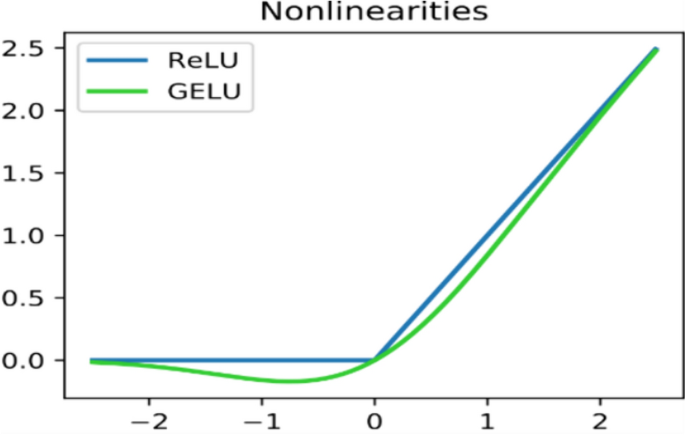
ReLU (coefficient of leakage α = 1) and GELU (learnable hyperparameters μ = 0, σ = 1) activation functions

This distribution is chosen after normalization layer since neuron’s input follow a normal distribution.
To make out it deterministic, expected value of transformation.
So
[41].
The graphical representation is depicting the nonlinearities of RELU and GELU in Fig. 4.
3.2.2 Normalization
Here, we have removed the batch normalization that was previously used in the U-Net architecture and replaced it with layer normalization in order to get around the drawbacks of batch normalization. It normalizes the activations in the feature direction rather than the mini-batch direction, which causes the network to pay more attention to the length of input to a particular layer. Because of this, the same procedures can be employed during the training process as well as during the inference process.
The computation shown below is carried out in order to normalize the layers of 2D images [42].
where x is the feature that a layer has computed and I(i, j) represent an index in the 2D image.
There is a four-dimensional vector indexing for the batch size N, the channel axis C, and the spatial height- H and breadth-B, respectively.
where layer normalization computes the \(\mu\) and \(\sigma\) along the C, H, W axis for each sample (Fig. 5).

Layer normalization along C, H and W axis [42]
The proposed architecture made use of AdamW optimizer to achieve competitive performance across denoising benchmarks while keeping the regular U-Net model's ease of use and efficacy intact (Figs. 6, 7).

UNet with Resnextify and IB modules architecture for low-dose CT image denoising

Internal multilayer perceptron (MLP) block procedure of convolution layer
4 Experiment and analysis
This section provides a detailed representation of the experimental setting including the implementation methodology, algorithm, datasets, evaluation metrics, ablation study and complexity.
4.1 Implementation details
Here, the proposed model’s performance is analyzed alongside that of many other state-of-the-art baselines. The training of the proposed method utilizes the following hardware environment on the experimental platform: The CPU is an Intel Core i9-9900 K@3.60 GHz and the operating system is Linux, memory is 15.3 GB for colab, 15.9 GB for Kaggle and graphic card is NVIDIA -SMI. CUDA version:12.0. In the Linux system environment, the Pytorch framework-2.0.0 with GPU: Tesla T4(Colab) is used to build and write the network framework. For training, 2378 distinct 512 × 512 pixel CT scans from the Mayo dataset were chosen by the experiment, testing and validation respectively 75%, 12% and 13%.
4.2 Algorithm
The following algorithm is used to implement the UNet with Resnextify and inverted bottleneck (IB) model for low dose computed tomography denoising, which results in significantly higher PSNR and SSIM values.

Algorithm: UNet with Resnextify and IB modules algorithm
4.3 Dataset
The dataset for this study was gathered from the TCIA- (The Cancer Imaging Archive) library that uses Digital Imaging and Communications in Medicine (DICOM) as its primary data storage format and for implementation purposes, these are converted to portable network graphics (PNG) for display [43]. This experiment made use of publicly available files from the 2016 NIH-AAPM Mayo Clinic LDCT Grand Challenge (https://www.apm.org/GrandChallenge/LowDoseCT/) [44]. This database contains information from 299 CT scans of the head, chest, and belly, 150 of which were performed on scanners manufactured by Siemens and 149 by GE scanners. In this dataset full dose (FD) data is achieved using 120kv and 200 quality reference mAs (QRM) and simulated data corresponding to 120 kv and 50 QRM for quarter dose data. This dataset has low- dose CT images with a slice diameter of 1 mm and 3 mm. It is frequently utilized for training and testing. For the experiment, 512 × 512-pixel CT images totaling 1819 are chosen as training data [44]. Data pertaining to images, such as patient outcomes, treatment information, genomes, and in-depth analysis, are also included. The TCIA collection contains a wealth of medical imaging resources that are put to good use in the study and treatment of illness [44].
4.4 Evaluation metrices
The experimental parameters for CT images based on UNET with resnextify and inverted bottleneck architecture are set as follows: the base learning rate α = 10–3, the convolution kernel in all layers has a size of 7 × 7.Number of epochs set to 120 and model is optimized using AdamW optimizer. In this architecture, weight Initialization is set as trunc. normal (0.02) for all the modules. To better assess the denoising effect of an algorithm on noisy CT images. We employed the peak signal-to-noise ratio (PSNR) measure as well as structural similarity. Description of each parameter is given below.
-
PSNR:
PSNR calculates peak signal to noise ratio between targeted image and calculated image. Higher value of PSNR indicates better quality of reconstructed images that is shown in Eq. (1) [45].
$$PSNR = 20\log_{10} \frac{255}{{\sqrt {{\frac{1}{mn}\sum_{i = 0}^{m - 1} \sum_{j = 1}^{n - 1} \left[ {I\left( {i,j} \right) - k\left( {i,j} \right)} \right]^2 }} }}$$(12)where I(i,j) = Real CT image of size m × n and K = Image after noise removal.
-
SSIM:
Structure similarity index for measuring similarity between two given images, it ranges from 0 to 1 where close to 1 means perfect match.
$$SSIM = \frac{{\left( {2\mu_x u_x , + C_1 } \right)\left( {2\sigma_{xx} , + C_2 } \right)}}{{\left( {\mu_x^2 + \mu_{x{\prime} }^2 + C_1 } \right)\left( {\sigma_x^2 + \sigma_{x{\prime} }^2 + C_2 } \right)}}$$(13)where \(\mu_{x{ }} ,u_x ,\) are mean values of images x and x′. \(\sigma_{x{ }} ,{ }\sigma_{x{^{\prime}}}\) are standard deviation of images x and x′. C1, C2 are constants (Fig. 8).
Fig. 8 
Figure a–c are low dose computed tomography Images before applying denoiser and after applying proposed model results are illustrated in figure d–f

4.5 Comparison with state-of -the art work
The shortcut link connects to convolutional and deconvolutional layers to increase the convergence speed. To verify the performance of proposed network, it is compared to standard algorithms, such as BM3D, K- K-singular value decomposition (SVD), Cycle-GAN and Cycle consistent adversial denoising network (CCADN) and semantic-aware knowledge-guided framework cycle generative adversarial network (SKFCycleGAN) [45, 46]. The experimental results on the Mayo dataset are illustrated in Table 1. This table is depicting the Comparison of different existed model’s result associated with the Mayo dataset. While the model on the S.no. 6 also used the U-Net with modified ConvNeXt model but the overall structure of the proposed model is completely different from the existing one to improve the performance such as: UNeXt model modified the dataset into 10 equal sized subsets by cross validation technique and only used one subset for the testing and remaining used for training while we have used 75% for training, 12% for testing and 13% for validation from the total image set. UNeXt model is divided into three modules shallow feature extraction – used sobel edge detector layer with fixed weighted kernel and combined into multi feature extraction block, Main feature extraction – In this module it has used CTNeXt where they have removed depth wise convolution layer by consecutive convolution layers with different kernel size (5,7,9…) while we have used resnextify for depth wise convolution to improve the performance of model (D-Conv 7 × 7) along with this to preserve the main features we have used inverted bottleneck structure. UNeXt reduced parameters while we have used some hyper parameters to enhance the network performance. UNeXt model used resolution of feature map—56,28,14,7 while we have used 256,128,64,32,16 and existing model used same structure of some blocks in down sampling and up sampling (conv and conv_Transpose) while we have applied different. UNeXt model didn’t provide the model complexity detail.
Proposed method gave the best performance for PSNR and SSIM with the values of 43.60 and 0.9761 respectively (Fig. 9).

Showing the growth of PSNR values and SSIM values over the different methodology
4.6 Ablation study
To demonstrate the effectiveness of each component, this research paper is conducted a series of ablation studies on a dataset. Major three factors are considered: 7 × 7 kernel (Increased kernel size with Patchify and linear normalization), Resnextifying and Inverted_bottelneck. This model consists of the U-Net branch and ConvNeXt branch with some hyperparameters. Each module contributes to the process of medical denoising in some way. In this work, several ablation analysis experiments were carried out in order to determine the relative importance of each contributing element to this model. The Mayo Dataset was subjected to an ablation analysis. As can be seen in Table 2, the modules belonging to the ConvNeXt branch had a more substantial impact than those belonging to the U-Net branch. Using this in-depth research, it has been seen that ConvNeXt-UNet was superior to U-Net + 7 × 7, which was superior to U-Net + Inverted_bottelneck, which was superior to U-Net + Resnextify. There are two major inferences to be made from this: First, in the context of low-dose computed tomography denoising, the whole model is an efficient and reliable approach to model selection. Second, the model versions proposed in this work are quite competitive in LDCT denoising tasks, proving once again the usefulness of the novel strategy taken (Fig. 10).

These figures a, b showing the ablation study evaluation using different modules added to U-Net model
4.7 Complexity
The network complexity E can be defined by the following equation [15].
where \(n_l\) is number of feature maps output by the \(l\) layer of the architecture and \(f_l\) is the size of layer convolution kernel. The complexity of ConvNeXt-UNet network in terms of parameters is depicting in Table 3 and it can be further improved. In this research, complexity is measured by using the number of parameters and size of parameters in megabyte. Complexity is quantified in this study by assessing the quantity and size of parameters, measured in megabytes. The UNet architecture utilizes depth-wise convolutions with 3 × 3 kernels, followed by ReLU activation, to perform spatial filtering on higher-dimensional pictures. Added best features of ConvNeXt model to base UNet mode. The complexity is determined by considering four stages. In the first level, a U-Net model with an enlarged kernel size of 7 × 7 is employed. The models are trained for approximately 120 epochs. It is worth noting that, for convolutional neural networks, the picture size does not affect the number of parameters. The size of the filter has a significant impact. That is clearly shown in the Table 4 with highest 156,739,715 parameters. In the subsequent stage, the utilization of the Inverted_bottelneck technique results in reduced memory usage and improved performance. In the third level, complexity is determined by considering only the resnextify feature, which significantly contributes to improving accuracy. Similar to an Inception module, it combines numerous transformations using a "split-transform-merge" approach, with branched routes within a single module. Furthermore, despite reducing parameters, relying solely on this approach fails to produce adequate results. However, in the fourth level, our model, employing concentrated and micro steps, achieved performance that reached the desired standard while maintaining an average level of complexity in terms of parameter count and size consumption (Fig. 11).

Figure a, b representing the complexity in terms of parameters and size in megabytes
5 Conclusion and future work
We studied ways to make the classic U-Net model more effective and came up with a revolutionary module adding up with it for the medical denoising of low-dose CT images. We chose the most useful aspects of the original resnextify—bottleneck from ConvNeXt model and adapted them so that they work with the U-Net architecture. Finally, this architecture is created by integrating the updated versions of modules and U-Net. By analysing the performance of each node in the network, we can determine that the following four factors contribute to the proposed method's ability to produce satisfactory outcomes: To extract more features and textures, we first create a lightweight U-Net contacting path using a modified convolutional block. Second, Resnext improves the trade-off between precision and FLOPs. To prevent data loss while keeping the input's spatial resolution, skip connections are utilized. We added a layer normalization to the network to address the over-fitting situation that could be generated by deepening the network. Lastly, PSNR and SSIM loss aids in tracking and improving the proposed network's performance. Extensive experimental findings on the Mayo dataset demonstrate that this model is extremely competitive for denoising the medical low-dose computed tomography (CT). Because of its streamlined plug-and-play architecture, the Resnextify-IB-UNet offers a significant benefit that is more adaptable. Additionally, this architecture is simpler to reproduce and deploy, which contributes to its overall usability and usefulness. We intend to conduct future investigations into the model improvement features, such as adding an attention mechanism, which would allow for a reduction in the number of hyperparameters. This would be accomplished by incorporating a parameter-free attention module such as SimAM, which stands for simple attention module, into the ConvNeXt backbone. This would allow for further enhancement of the performance of the suggested network and a reduction in the complexity of the model. In addition to this, it is simple to create a quick model for noise reduction by determining the significant similarities that exist between LDCT and NDCT images. For example, we could include the YOLO series in this model. In addition, we may improve our method and extend its application to more CT image processing tasks, such as the diagnosis of lung cancer, the segmentation of public and clinical datasets, and the correction of geometric errors.
References
Shah NB, Platt SL (2008) ALARA: is there a cause for alarm? Reducing radiation risks from computed tomography scanning in children. Curr Opin Paediatr 20:243–247. https://doi.org/10.1097/mop.0b013e3282ffafd2
Chen Hu et al (2017) Low-dose CT via convolutional neural network. Biomed Opt Express 8(2):679–694. https://doi.org/10.1364/BOE.8.000679
Shan H et al (2018) 3-D convolutional encoder-decoder network for low-dose CT via transfer learning from a 2-D trained network. IEEE Trans Med Imaging 37:1522–1534. https://doi.org/10.1109/TMI.2018.2832217
Shan H et al (2019) Competitive performance of a modularized deep neural network compared to commercial algorithms for low-dose CT image reconstruction. Nat Mach Intell 1:269–276. https://doi.org/10.1038/s42256-019-0057-9
Wu D et al (2017) A cascaded convolutional nerual network for X-ray low-dose CT image denoising. arXiv:1705.04267
Wang G, Ye JC, Mueller K, Fessler JA (2018) Image reconstruction is a new frontier of machine learning. IEEE Trans Med Imaging 37:1289–1296. https://doi.org/10.1109/TMI.2018.2833635
Zhao H, Gallo O, Frosio I, Kautz J (2017) Loss functions for image restoration with neural networks. IEEE Trans Comput Imaging 3:47–57. https://doi.org/10.1109/TCI.2016.2644865
Yuan H et al (2018) SIPID: a deep learning framework for sinogram interpolation and image denoising in low-dose CT reconstruction. In: IEEE 15th international symposium on biomedical imaging, pp 1521–1524
Kakhandaki N, Kulkarni SB (2023) Classification of brain MR images based on bleed and calcification using ROI cropped U-Net segmentation and ensemble RNN classifier. Int J Inf Tecnol 15:3405–3420. https://doi.org/10.1007/s41870-023-01389-2
Mao X-J et al (2016) Image restoration using very deep convolutional encoder-decoder networks with symmetric skip connections. In: Neural information processing systems
Chen H et al (2017) Low-dose CT with a residual encoder–decoder convolutional neural network. IEEE Trans Med Imaging 36:2524–2535. https://doi.org/10.1109/TMI.2017.2715284
Xie J et al (2012) Image denoising and inpainting with deep neural networks. In: Neural information processing systems. https://api.semanticscholar.org/CorpusID:13852540
Li M et al (2020) SACNN: self-attention convolutional neural network for low-dose CT denoising with self-supervised perceptual loss network. IEEE Trans Med Imaging 39:2289–2301. https://doi.org/10.1109/TMI.2020.2968472
Sheikh BUH, Zafar A (2024) White-box inference attack: compromising the security of deep learning-based COVID-19 diagnosis systems. Int J Inf Technol 16:1475–1483. https://doi.org/10.1007/s41870-023-01538-7
Zhang H et al (2023) BCU-Net: Bridging ConvNeXt and U-Net for medical image segmentation. Comput Biol Med 159:106960. https://doi.org/10.1016/j.compbiomed.2023.106960
Liu Z, Mao H et al (2022) A ConvNet for the 2020s. In: IEEE/CVF conference on Computer Vision and Pattern Recognition (CVPR), pp 11966–11976. https://doi.org/10.1109/CVPR52688.2022.01167
Yuan J et al (2020) HCformer: hybrid CNN-transformer for LDCT image denoising. J Digit Imaging 36:2290–2305. https://doi.org/10.1007/s10278-023-00842-9
Qu H, Liu K, Zhang L (2024) Research on improved black widow algorithm for medical image denoising. Sci Rep 14:2514. https://doi.org/10.1038/s41598-024-51803-3
Sarwar A, Ali M, Manhas J et al (2020) Diagnosis of diabetes type-II using hybrid machine learning based ensemble model. Int J Inf Technol 12:419–428. https://doi.org/10.1007/s41870-018-0270-5
Xiong L, Li N et al (2023) Re-UNet: a novel multi-scale reverse U-shaped network architecture for low-dose CT image reconstruction. Nuclear Technology Medical Transformation. SSRN: https://ssrn.com/abstract=4426158
Zhang K, Zuo W, Zhang L (2018) FFDNet: toward a fast and flexible solution for CNN-based image denoising. IEEE Trans Image Process 27:4608–4622. https://doi.org/10.1109/TIP.2018.2839891
Yang D, Sun J (2018) BM3D-Net: a convolutional neural network for transform-domain collaborative filtering. IEEE Signal Process Lett 25:55–59. https://doi.org/10.1109/LSP.2017.2768660
Tai Y et al (2023) MemNet: a persistent memory network for image restoration. ArXiv, pp 4549–4557. https://api.semanticscholar.org/CorpusID:8550762
Esmaeilzadeh Asl S et al (2023) Brain tumors segmentation using a hybrid filtering with U-Net architecture. Multimodal MRI volumes. Int J Inf Technol. https://doi.org/10.1007/s41870-023-01485-3
Kanwade AB, Sardey MP, Panwar SA et al (2024) Combined weighted feature extraction and deep learning approach for chronic obstructive pulmonary disease classification using electromyography. Int J Inf Technol 16:1485–1494. https://doi.org/10.1007/s41870-023-01498-y
Zhu J, Yao C et al (2022) MRDA-Net: multiscale residual dense attention network for image denoising. In: Advances in artificial intelligence and security ICAIS. Communications in Computer and Information Science. Springer, Cham. https://doi.org/10.1007/978-3-031-06767-9_18
Zheng Ao et al (2020) A dual-domain deep learning-based reconstruction method for fully 3D sparse data helical CT. Phys Med Biol 24:245030. https://doi.org/10.1088/1361-6560/ab8fc1
Sajedi H, Mohammadipanah F (2024) (2024) Global data sharing of SARS-CoV-2 based on blockchain. Int J Inf Tecnol 16:1559–1567. https://doi.org/10.1007/s41870-023-01431-3
Parthasarathy V, Saravanan S (2024) Computer aided diagnosis using Harris Hawks optimizer with deep learning for pneumonia detection on chest X-ray images. Int J Inf Technol 16:1677–1683. https://doi.org/10.1007/s41870-023-01700-1
Feng Z, Li Z, Cai A, Li L, Yan B, Tong L (2020) A preliminary study on projection denoising for low-dose CT imaging using modified dual-domain U-net. In: 3rd International Conference on Artificial Intelligence and Big Data (ICAIBD), Chengdu, China, pp 223–226. https://doi.org/10.1109/ICAIBD49809.2020.9137456
Chaurasiya R, Ganotra D (2023) Deep dilated CNN based image denoising. Int J Inf Technol 15:137–148. https://doi.org/10.1007/s41870-022-01125-2
Dong J et al (2019) A deep learning reconstruction framework for X-ray computed tomography with incomplete data. PLoS ONE 11:e0224426. https://doi.org/10.1371/journal.pone.0224426
Lee H, Lee J, Kim H, Cho B, Cho S (2019) Deep-neural-network-based sinogram synthesis for sparse-view CT image reconstruction. IEEE Trans Radiat Plasma Med Sci 3:109–119. https://doi.org/10.1109/TRPMS.2018.2867611
Kida S et al (2018) Cone beam computed tomography image quality improvement using a deep convolutional neural network. Cureus. https://doi.org/10.7759/cureus.2548
Liu P, Zhang H, Zhang K et al (2018) Multi-level wavelet-CNN for image restoration. In: IEEE/CVF Conference on Computer Vision and Pattern Recognition Workshops (CVPRW), pp 886–88609. https://doi.org/10.1109/CVPRW.2018.00121
Chhikara R, Sharma P, Chandra B et al (2023) Modified Bird Swarm Algorithm for blind image steganalysis. Int J Inf Technol 15:2877–2888. https://doi.org/10.1007/s41870-023-01355-y
Luo Y, Majoe S, Kui J, Qi H, Pushparajah K, Rhode K (2021) Ultra-dense denoising network: application to cardiac catheter-based X-ray procedures. IEEE Trans Biomed Eng 68:2626–2636. https://doi.org/10.1109/TBME.2020.3041571
Mohd Sagheer SV, George SN (2019) Denoising of low-dose CT images via low-rank tensor modeling and total variation regularization. Artif Intell Med 94:1–17. https://doi.org/10.1016/j.artmed.2018.12.006
Hong S, Wang A, Zhang X, Gui Z (2018) Low-dose CT image processing using artifact suppressed total generalized variation. J Netw Intell 3(1):26–49
Ronneberger et al (2015) U-Net: convolutional networks for biomedical image segmentation. In: Medical Image Computing and Computer-Assisted Intervention—MICCAI 2015. Lecture notes in computer science. Springer, Cham. https://doi.org/10.1007/978-3-319-24574-4_28
Hendrycks D, Gimpel K (2016) Gaussian error linear units (GELUs). ArXiv. http://arxiv.org/pdf/1606.08415v3
Ba JL, Kiros JR, Hinton GE (2016) Layer normalization. cite arXiv:1607.06450
Kandarpa VSS, Bousse A, Benoit D, Visvikis D (2021) DUG-RECON: a framework for direct image reconstruction using convolutional generative networks. IEEE Trans Radiat Plasma Med Sci. https://doi.org/10.1109/TRPMS.2020.3033172
McCollough CH et al (2017) Low-dose CT for the detection and classification of metastatic liver lesions: results of the 2016 low dose CT grand challenge. Med Phys 44:e339–e352. https://doi.org/10.1002/mp.12345
Parmar JM, Patil SA (2013) Performance evaluation and comparison of modified denoising method and the local adaptive wavelet image denoising method. In: International Conference on Intelligent Systems and Signal Processing (ISSP), Vallabh Vidyanagar, India, pp 101–105. https://doi.org/10.1109/ISSP.2013.6526883
Tan C et al (2022) A selective kernel-based cycle-consistent generative adversarial network for unpaired low-dose CT denoising. Precis Clin Med. https://doi.org/10.1093/pcmedi/pbac011
Yan K, Wang X, Lu L, Summers RM (2017) Deeplesion: automated deep mining, categorization and detection of significant radiology image findings using large-scale clinical lesion annotations. ArXiv preprint. https://doi.org/10.48550/arXiv.1710.01766
Unal MO et al (2014) Proj2Proj: self-supervised low-dose CT reconstruction. PeerJ. Comput Sci 10:e1849. https://doi.org/10.7717/peerj-cs.1849
Moen T, Chen B, David Holmes III, Duan X, Zhicong Yu, Lifeng Yu, Leng S, Fletcher J, McCollough C (2020) Low dose CT image and projection dataset. Med Phys 48:902–911. https://doi.org/10.1002/mp.14594
Zhang B, Zhang Y et al (2024) Denoising swin transformer and perceptual peak signal-to-noise ratio for low-dose CT image denoising. Measurement. https://doi.org/10.1016/j.measurement
Jia L, Huang A, He X et al (2023) A residual multi-scale feature extraction network with hybrid loss for low-dose computed tomography image denoising. SIViP. https://doi.org/10.1007/s11760-023-02809-3
https://www.cirsinc.com/products/all/24/electron-density-phantom/
Xia Z et al (2023) Dynamic controllable residual generative adversarial network for low-dose computed tomography imaging. Quant Imaging Med Surg 13:5271–5293. https://doi.org/10.21037/qims-22-1384
Trung NT, Trinh DH, Trung NL et al (2022) Low-dose CT image denoising using deep convolutional neural networks with extended receptive fields. SIViP. https://doi.org/10.1007/s11760-022-02157-8
https://imaging.cancer.gov/informatics/cancer_imaging_archive.htm
Chi J, Wu C, Yu X, Ji P, Chu H (2020) Single low-dose CT image denoising using a generative adversarial network with modified U-Net generator and multi-level discriminator. IEEE Access 8:133470–133487. https://doi.org/10.1109/ACCESS.2020.3006512
Liu Y, Chen Y, Chen P, Qiao Z, Gui Z (2019) Artifact suppressed nonlinear diffusion filtering for low-dose CT image processing. IEEE Access 7:109856–109869. https://doi.org/10.1109/ACCESS.2019.2933541
Trine H, Trygve L et al (2007) Three-dimensional atlas system for mouse and rat brain imaging data. Front Neuroinform. https://doi.org/10.3389/neuro.11.004.2007
Gupta H, Jin KH et al (2018) CNN-based projected gradient descent for consistent CT image reconstruction. IEEE Trans Med Imaging 37:1440–1453. https://doi.org/10.1109/TMI.2018.2832656
Author information
Authors and Affiliations
Corresponding author
Ethics declarations
Conflict of interest
The authors declare that they have no conflict of interest.
Rights and permissions
Springer Nature or its licensor (e.g. a society or other partner) holds exclusive rights to this article under a publishing agreement with the author(s) or other rightsholder(s); author self-archiving of the accepted manuscript version of this article is solely governed by the terms of such publishing agreement and applicable law.
About this article

Cite this article
Chauhan, S., Malik, N. & Vig, R. UNet with ResNextify and IB modules for low-dose CT image denoising. Int. j. inf. tecnol. 16, 4677–4692 (2024). https://doi.org/10.1007/s41870-024-01898-8
Received:
Accepted:
Published:
Issue Date:
DOI: https://doi.org/10.1007/s41870-024-01898-8